
Abstract
Marine controlled source electromagnetic (MCSEM) is an efficient technique for the marine hydrocarbon explorations. Over the past decades, the numerical research on induced polarization (IP) effects in offshore environment is still a intensive topic. Presented here are the results of a 3D new MCSEM forward for IP modeling exercise with the intent of demonstrating the valuable applications of this developed methodology. By using the finite volume method, an analysis on amplitude and phase of electromagnetic field due to the varying IP parameters within the Cole-Cole model is presented. The numerical examples demonstrate that the amplitude and the phase of electromagnetic field due to the IP effects are subtle, and it is difficult to detect the reservoir hydrocarbon object using such subtle amplitude and phase directly in offshore environment. Based on the assumption that most IP phase spectra can be represented by a linear function of the logarithm of frequency, we apply a two-frequency IP phase decoupling technique for MCSEM data interpretation, which is a plausible example. Numerical IP phase decoupled results for a thin reservoir hydrocarbon object demonstrate the efficiency of the two-frequency IP decoupled technique for MCSEM data interpretation.
Keywords
Introduction
Marine controlled source electromagnetic (MCSEM) method, used for about a few years mainly for commercial reservoir appraisal and hydrocarbon exploration, has become well established as an important geophysical tool in the offshore environment [1,2]. This method has featured much more and more importantly, which behaves so very differently with the sensitiveness to high electrical resistivity and a much better intrinsic resolution than the primary nonseismic methods (such as gravity and magnetic surveying) used in current offshore exploration. Some research directions about this method presently include developing available 3D anisotropic forward and inversion methods, the thin resistive layer detection, equipment improvements and so on [3]. But the induced polarization (IP) is rare occurred in surveys and publications associated with MCSEM. One of the reasons for this phenomenon may be that IP measured data were inconclusive resistivity data showed good results, i.e., in land exploration, the IP effects are measured in less than 30% of the surveys over known hydrocarbon accumulations [4]. For the offshore IP measurements, the IP effect is a different physical property than those properties in land exploration mainly as a consequence of two aspects associated with the physics of the method: the highly conductive seawater and the effective marine IP data-gathering [5]. Even so limited by the above difficulties, Scott et al. [6] pioneered the application of a surface-towed induced polarization streamer in a marine environment [6]. Although the initial IP results were discouraging due to high noise levels, Wynn et al. [7] carried out the induced polarization measurements successfully to sea-floor mineral exploration for titanium geophysics [7].
For the reservoir appraisal and hydrocarbon exploration in offshore environment, some incentives exist to use the IP method offshore [8]. The unknown substantial reservoir resources are located in million square miles of exclusive economic zones. On land, these reservoir zones have been shown to give rise to substantial IP effects. The rise in CSEM exploration at water depths greater than 1000 m in the Gulf of Mexico came in 2006. It can be seen that explorations at these depths are available as tension-leg platforms and other deep water technologies and equipments were developed [9].
Although a finite-element forward code [10], a 2D finite-difference forward and inverse code [11] are applied for CSEM, the large computation cost in finite-element method [12] and the accuracy restriction on finite-difference method make them difficult to be widely use [13,14]. The finite-volume method is designed to achieve the balance between the large computation cost and low accuracy. This method only needs to calculate the field at discrete points, but considers the relationship of the discrete pints in a controlled volume. Thus, the finite-volume method has a similar computation cost with finite-difference method but a higher accuracy. In our work, a 3D finite-volume forward code for MCSEM is developed to calculate IP effects associated with MCSEM. In this paper, we will first analyze the IP effect anomalies in MCSEM using this kind of 3D finite volume method based on the typical Cole-Cole model parameters (chargeability, time constant and frequency dependence).
A fundamental problem for using the IP method in sea water is that the IP response of the medium is subtlest generally in the order of the resistivity signal. The IP effect is exacerbated by electromagnetic (EM) coupling when its contribution is large compared to the IP signal. EM coupling would arouse a profound effect, and such effect will be increased when the measurement is carried out over a conductive environment. Some principal directions of research on EM coupling removal have evolved over the past decades [15–17]. We won’t give the judgment here since all the methods have the advantages and disadvantages. For the details, the readers can refer to the references [15]. Although all those methods are approximate, they are used successfully in different applications [18–21]. In our work, a decoupling method based on the assumption that the IP phase is a linear function of the logarithm at frequency and can be presented by two or three frequencies, is used to remove the EM coupling associated with MCSEM. Although Kulikov and Shemyakin used the two-frequency IP approach for detection of ore deposits [22], Davydycheva et al. concentrated on its application for the oil search [23]; To our knowledge, such a method for IP effects decoupling using electromagnetic field in offshore environment has not been reported previously.
Formulations
In frequency domain, partial differential equation (PDE) in electromagnetic wave governed with conductivity σ, and without considering permeability (𝜇 = 𝜇0) is governed by the following equation
From (1), one can find it is singular at the source point, in order to solve this problem, we introduce into a reference model σ0 (for example, σ0 is a conductivity constant). The primary fields

The sketch of control volume (left) and Yee grid (right).
We also have
Using the Gauss theorem
It is observed from formulation (5) that one can use finite volume method to discretize the electromagnetic field by making up a finite volume around the calculated point. To solve formulation (5), we first discretize the electromagnetic field at Yee grid system, in which the electric fields are located at the center of each edge of cubic cell while the magnetic fields are located at the center of the surface of cubic cell, as shown in Fig. 1. In this way, formulation (5) can be discretized into scale linear equations in three directions.
When considering the IP effects in MCSEM, the complex resistivity are presented by typically Cole-Cole model in frequency domain is used. The complex resistivity (CR) method has been widely applied in minerals exploration, here, we apply it in MCSEM for reservoir exploration. According to [17], the complex resistivity of sediment rock can be defined by Cole-Cole model as
To simulate the electromagnetic field with considering IP effects, one only need to replace the conductivity in formulation (5) with the complex conductivity in formulation (7), and then solve the linear equations using Quasi Minimum Residual Error method. The variations of chargeability, time constant and frequency dependence are considered in this paper.
To validate the efficiency of the 3D MCSEM code presented in this paper, we first construct a corroboration with the analytic solution basing on a 1D two-layer homogeneous medium model [24], when the first layer is seawater (3.3 S/m) and the second layer is seafloor sediments (1.0 S/m). Actually this 1D homogeneous model is similar with the basic model shown in Fig. 2, except that the reservoir object is absent. For simplicity, an horizontal electric dipole is located at x = −500 m on the seabed, and the frequency is 0.25 Hz. Some electric field recorders are located on the seabed from −1000
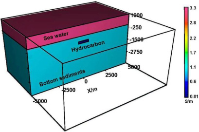
The sketch of three dimensional layered medium consists of a rectangle thin hydrocarbon layer.
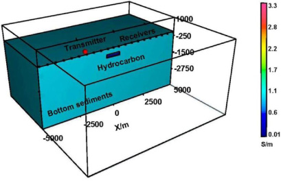
The sketch of a model stripped the sea water and a measurement system for MCSEM.
Figure 4 and Fig. 5 are the numerical comparisons of electric field results between the 3D finite-volume forward code and the 1D analytic solution. It is seen that the results from those two methods are matching quire well except that the zone near the source point, which maybe caused by the coarse grid subdivision. For the MCSEM, the far field is essential for exploration, which is the part we focus on in this work. The field ratio (Fig. 4) and the phase difference (Fig. 5) between the two result sets also demonstrate the efficiency of the 3D finite-volume forward code.
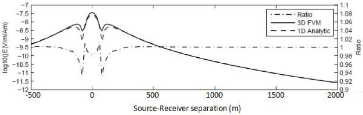
Numerical horizontal electric field for a 1D two-layer homogeneous model with the 3D FVM code and the 1D analytic solution.
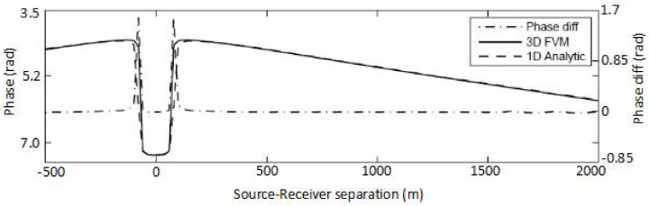
Numerical phase of the horizontal electric field for a 1D two-layer homogeneous model with the 3D FVM code and the 1D analytic solution.
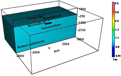
In this section, we consider a three dimensional two-layer medium with conductivities of 3.3 S/m (sea water) and 1.0 S/m (sediments), embedded a reservoir object with conductivity of 0.02 S/m, as shown in Fig. 2. The depth for the seabed is 1000 m. Actually the ability to detect reservoirs in water depths larger than 1000 m coincides with the rise in producing CSEM exploration (Minerals Management Service, 2010). The reservoir presents a thin layer filled with hydrocarbon with a size of 1000 m × 1000 m × 200 m. In such a marine environment, seafloor sediments with a thickness of 300
Amplitude and phase analysis
Amplitude and phase of the electromagnetic field are direct approaches to analyze the anomaly from IP effects for reservoir object. To do this, we construct a case with regular IP parameters for measurement. In microcosm, the IP effects of reservoir object are come from multiphase medium (oil, oil-water, water, solid) with some electrochemical reactions. This kind of IP mechanism is difficult and challenging in geophysical computation right now. The Cole-Cole model is a equivalent circuit for such a IP mechanism, where the complex impedance (referred the zero frequency, the time constant, the chargeability and the frequency dependence) simulates the multiphase medium interface. In general, the Cole-Cole relaxation model coincides with the IP spectra. The frequency dependence of most IP responses has a mean value near 0.25 with a range between 0.1 and 0.6 Theoretical values for the time constant and the chargeability are quire different in many exploration cases, which is also demonstrated in some field explorations. In this regard, the chargeability of hydrocarbon reservoir object is 0.5, the time constant is 0.1 and the frequency dependence is 0.5 in our work. Based on the above model setup, the frequency for the source is 0.5 Hz. To outstand the IP effects, the amplitude and phase of the electromagnetic field with (High resistivity with IP) and without (High resistivity) considering IP effects are calculated and shown in Fig. 4. The amplitudes are normalized with those results calculated in a two-layer medium (sea water and sediments) without reservoir object.
As shown in Fig. 4, the normalized amplitudes of electric and magnetic field have anomalous jumps at 1500 m and 2500 m, the range between those two jumps marches well with the range of reservoir object in source-receiver separation axis. When the receivers are far from the reservoir object, the normalized amplitudes of field for both with and without considering IP effects approach to 1, it is reasonable as the electromagnetic power would be attenuated fast in offshore environment. The phase of the electromagnetic field for both with and without considering IP effects have similar anomaly with those anomaly presented in amplitude, shown in Fig. 4. Except that the phase curves parallel with each other started from 2000 m to large source-receiver separation. Although the maximum value in amplitude is up to 35% in normalized percentage, however, the differences in amplitude and phase between with and without considering IP effects are less than 10%. Thus, this analysis in amplitude and phase demonstrates that one hopes to detect reservoir object based on those subtle differences directly is not advisable, especially for the realistic MCSEM data which contaminated noises (e.g., random and coherent noises).
Analysis based on varying IP parameters
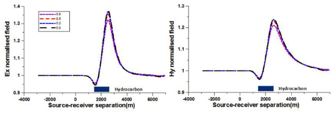
To analyze the anomaly of electromagnetic field with considering varying IP parameters in offshore environment, we construct three cases with different chargeability, time constant and frequency dependence, respectively. For conventional consideration, here, the different chargeability are chose to be 0.0, 0.2, 0.5 and 0.8; the varying time constant are 0.1, 1, 10, 100 second, and the frequency dependence are 0.25, 0.5 and 1.0. When one of the IP parameters varies with different values, we assume that the other three IP parameters are same with those parameters in the last case shown in Section 3.1. As the analysis points out in the above section, the amplitude anomaly is similar with those anomaly presented in phase, thus, for simplicity, we just post the results of amplitude in this section.

Numerical amplitude and phase of electromagnetic field for a high resistivity reservoir model with IP effects normalized by corresponding components of a two-layer (sea water and sediments) background medium.
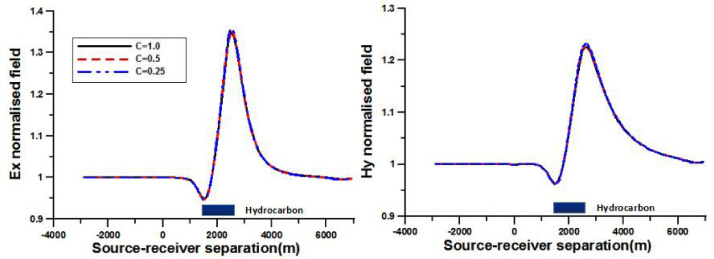
The normalized amplitude for electric and magnetic field with considering varying IP parameters are shown in Fig. 5, Fig. 6 and Fig. 7. Again, one can observe two anomalous jumps in all those three figures, which agree with the edges of reservoir object in source-receiver separation axis (1500 m and 2500 m). However, the differences in the normalized amplitude of electromagnetic field between different chargeability are small, even for those cases with four times in chargeability (m = 0.8 and 0.2). To show the details, we also present the amplitude of electromagnetic field normalized with those results without considering IP effects (m = 0.0) in Fig. 8. As one can see that the maximum in the normalized amplitude is less than 10%. While the differences in the normalized amplitude between varying time constant and frequency dependence are negligible for the model shown in this paper. There have two main reasons accounting for this phenomenon. The first reason is that the electromagnetic response is subtle in offshore environment. It is difficult to identify the IP effects based on such a subtle signal in amplitude directly. The other one is that the complex resistivity presented by a Cole-Cole model in frequency domain is approximate in mathematics. In general, the IP effects are more complicated than an application of Cole-Cole model. The above analysis indicates that it is impossible to detect reservoir object in offshore environment by using the electromagnetic field with considering IP effects directly.
Numerical amplitude and phase of electromagnetic field with varying chargeability for a high resistivity reservoir model with IP effects normalized by corresponding components of a two-layer (sea water and sediments) background medium.
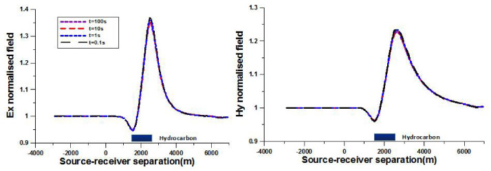
Numerical amplitude and phase of electromagnetic field with varying time constants for a high resistivity reservoir model with IP effects normalized by corresponding components of a two-layer (sea water and sediments) background medium.
In a narrow frequency band, Hallof [18] assumed that the IP phase spectra can be approximate constant. However, as shown in the references [16], the phase spectra of several mineralized samples measured in the laboratory did not strictly support his assumption. Liu [21] assumed and confirmed that the IP phase is a linear function of the logarithm of frequency, such an approximation is more realistic and also more consistent with the Cole-Cole model. Here, we follow Liu [21] and apply a two-frequency IP decoupling technique in MCSEM data. By doing this, we wish to seek the possibility of detecting reservoir object in offshore environment by using IP phase.
For simplicity, this paper just presents a brief overview for a two-frequency IP decoupling algorithm. For details, the readers can refer to the references [19]. Assuming that the phase of total field consists of IP and inductive component, those two phase components can be defined as
This formulation give us a possibility of obtaining the approximate IP phase from the total phase of total field using adjacent two frequencies. Theoretically, the FVM method presented in this paper would be used to provide electromagnetic field at any frequency in the offshore environment. However, the low frequency range (0.1–10 Hz) is dominating in practical explorations. As demonstrated in above numerical analysis, the IP effect is dominating at a suitable source-receiver separation, so that the reservoir object is located in the best intensity of illumination in the configuration. For those reasons, we discuss the IP decoupling below.
To verify the efficiency of this two-frequency decoupling technique in marine hydrocarbon exploration, we first analyze the phase spectra at two special receivers for numerical investigation, as shown in Fig. 9. The two receivers are defined as receiver A and receiver B, in which the receiver A is located above the center of the reservoir object (2000 m in Source-receiver separation axis) and would take the dominant IP effects, while the receiver B is located far from the reservoir object (500 m in Source-receiver separation axis) and would ignore IP effects. The decoupled results in the receiver B is also considered as the standard background result for comparison with those in receiver A. In this section, all the numerical cases are based on the model and measurement system shown in Fig. 3.
Numerical amplitude and phase of electromagnetic field with varying frequency dependencies for a high resistivity reservoir model with IP effects normalized by corresponding components of a two-layer (sea water and sediments) background medium.
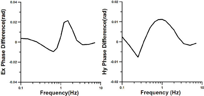
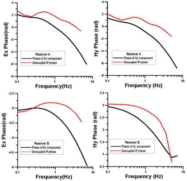
Figure 10 shows the theoretical IP decoupled results for a reservoir object embedded in a two-layer (sea water and sediments) background medium without considering IP effects at receiver A and receiver B. Note that the IP decoupled phase at receiver B in this case is similar with those cases in the homogeneous layered background medium without reservoir. There have small differences in IP decoupled phase at receiver A compared to those results at receiver B. Such differences may be caused by pure induction from the reservoir object and suggest that this applied two-frequency decoupled scheme is actually an approximate technique. When without the IP phase component, the IP decoupled results would be negligible, as shown in Fig. 11, the differences between the decoupled results of a reservoir object without considering IP effects and a two-layer background medium are less than 0.02 rad. This may contaminates a negligible error, though the error is neither a constant nor a linear function of frequency.
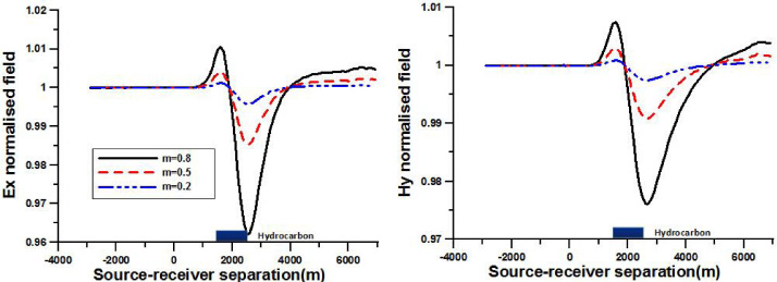
Numerical amplitude and phase of electromagnetic field with varying chargeability for a high resistivity reservoir model with IP effects normalized by corresponding components of a high resistivity reservoir model.
The sketch of a model and a measurement system for testing of two-frequency IP decoupling technique.
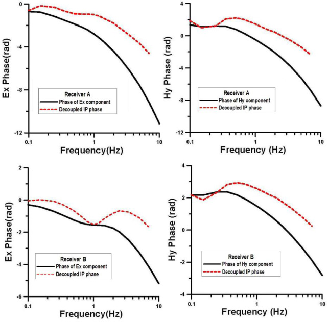
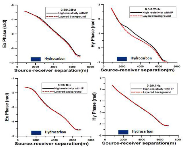
The theoretical IP decoupled results for a reservoir object embedded in a two-layer (sea water and sediments) background medium with considering IP effects are presented in Fig. 12. One can note that the IP decoupled phase in electric field are negative value at receiver B and become positive at receiver A, while the IP decoupled phase in magnetic field are positive value at receiver B and gradually change from positive to negative at receiver A. These decoupled characteristics would be used to identify whether the reservoir being with IP effects or not. The decoupled results shown in Fig. 12 also indicate that the amplitude of decoupled IP phase are advisable to be measurable and can be robust separated.
Theoretical IP decoupled results of a high resistivity reservoir without IP effects at receiver A and receiver B.
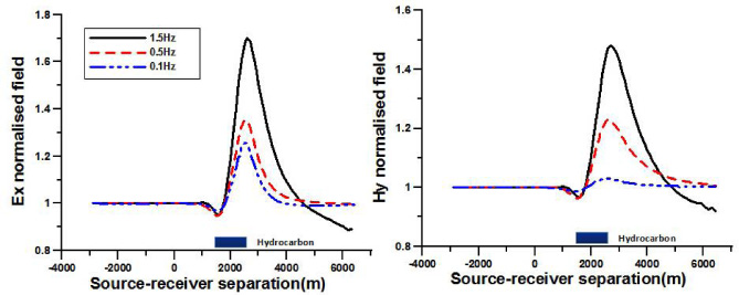
Based on the phase spectra shown in Fig. 12, we also present the normalized amplitude of electromagnetic field versus source-receiver separation at three frequencies (0.1, 0.5 and 1.5 Hz), shown in Fig. 13. One can observe that the anomalous amplitude increase along with the frequency axis. In particular, the normalized value is about 20% for electric field and is less than 10% for magnetic field at 0.1 Hz, while the normalized values are up to 70% and 50% for electric and magnetic field at 1.5 Hz respectively. A decline in normalized amplitude also would be seen after 5000 m in source-receiver separation at 1.5 Hz. Those anomalous characteristics suggest that a proper frequency range for IP phase decoupling is 0.1–1.5 Hz.
Numerical comparison of the differences between the phases decoupled results of a high resistivity reservoir model without IP effects and those in a two-layer background medium at receiver B.
And then, We calculate the decoupled phase along a surveying line with four groups of frequency pairs (0.5/0.25 Hz, 0.5/0.1 Hz, 1.5/0.5 Hz and 1.5/0.1 Hz), shown in Figs 14 and Fig. 15. It is obvious that, the decoupled IP phase of electromagnetic field are more sensitive to the polarized reservoir object (1500
Theoretical IP decoupled results of a high resistivity reservoir model with IP effects at receiver A and receiver B.
Numerical amplitude of electromagnetic field for a high resistivity reservoir model with IP effects normalized by corresponding components of a high resistivity reservoir model.

Theoretical IP decoupled results of a high resistivity reservoir model with IP effects at two groups of different frequencies.
Theoretical IP decoupled results of a high reservoir resistivity model with IP effects at two groups of two-frequency.
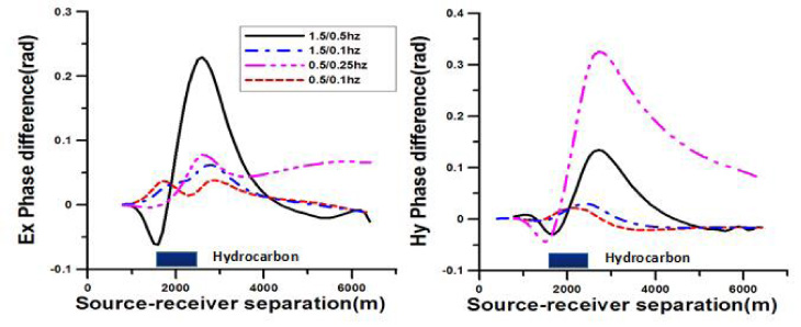
Numerical comparison of the differences between the decoupled phase results of a high resistivity reservoir model with IP effects at four groups of two-frequency.
A new 3D FVM program for MCSEM forward is introduced and presented in this paper. With the efficient simulated tool, the present study has characterized the IP effects of MCSEM field based on the varying Cole-Cole model parameters (chargeability, time constant and frequency dependence) over a marine 3D hydrocarbon model. The effectiveness of a two-frequency IP phase decoupling technique in reservoir hydrocarbon exploration is demonstrated by numerical modeling.
The analysis on numerical case study shown that two anomalous jumps in amplitude and phase curves are marched quite well with the distribution of reservoir object in source-receiver separation axis. Although the maximum value in amplitude and phase is up to 35% in normalized percentage, the differences in amplitude and phase between with and without considering IP effects are less than 10%. Study in the normalized amplitude of electromagnetic field with considering varying IP parameters in complex resistivity, also indicated that the anomaly in electromagnetic field due to the varying IP parameters is subtle and negligible. Thus, one wishes to detect reservoir object using those subtle IP signal in amplitude and phase of electromagnetic field directly is not advisable, especially for the realistic MCSEM data which contaminated noises usually.
A proper two-frequency decoupling technique is applied to decouple IP phase from electromagnetic field in offshore environment, which is a possible trial of reservoir exploration. The effectiveness and accuracy of the decoupling technique were justified by numerical decoupled results over a two-layer (sea water and sediments) background medium, a thin reservoir hydrocarbon object (high resistivity model compared to background medium) with and without considering IP effects. Numerical comparisons of the IP decoupled phase at four two-frequency pairs demonstrated that 2
Footnotes
Acknowledgements
This work is supported by Natural Science Foundation of China (No. 41604097, No. 41874085), Guangxi Natural Science Foundation (No. 2016GXNSFBA380195, No. 2018GXNSFAA281028), Guilin University of Technology research funding (002401003503, 002401003514).