Ion flow field distribution near the crossing of two circuit UHVDC transmission lines

Abstract

The 3D upstream FEM is applied to calculate the ion flow field near the crossing of two circuit ±800 kV UHVDC transmission lines. In order to deal with the interaction of two circuit lines, an improved space charge density correcting treatment on the conductor surfaces is proposed. Compared with the traditional method, the conductor surface electric fields could be closer to the corona onset electric fields by using the improved correction treatment. Then, an experimental platform is established in the laboratory to testify the calculation method. Comparison of the calculated and measured ground-level ion current density proves the validity of calculation method. Finally, the distribution characteristics of space charge density and electric field strength near the crossing area are analyzed. The crossing structure of bipolar HVDC lines improves the corona discharge level in the opposite polarity crossing area significantly.

Keywords

Corona discharge ion flow field HVDC lines crossing upstream FEM

1. Introduction

In recent years, a lot of ultra-high-voltage direct current (UHVDC) transmission projects have been put into operation or under construction in many countries. The length of UHVDC lines usually reaches to 2000 km and above. Therefore, the crossing of two circuit UHVDC lines might become a new problem in the engineering. Corona discharge occurs when the electric field around the surface of high voltage lines exceeds the corona onset value. Ions generated by corona move under the force of DC electric field, and then influence the electric field in the space, which is known as ion flow field problem [1,2]. Because of the effect of ions, predicting the electric field near HVDC lines is more difficult than that near high-voltage alternating current (HVAC) lines [3,4].

The basic principle of ion flow field calculation is to solve Poisson’s equation and ion transport equation. The ion flow field calculation methods can be divided into two categories, i.e., the Lagrange description and the Euler description. Methods based on Lagrange description include flux tracing method (FTM) [5–7] and method of characteristics (MOC). F. Xiao et al. calculated the ground-level ion flow field under cross-over ±800 kV lines by 3D MOC [8]. The Lagrange methods are good at dealing with open domain problems and have the advantages of stability. The main methods in Euler description are mesh-based methods, such as upstream finite element method (upstream FEM) [9–12], hybrid finite element method and finite volume method (FEM–FVM) [13,14], etc. X. Zhou et al. simulated the hybrid electric field near the cross-over HVDC and HVAC lines by FEM–FVM [13]. Upstream FEM is a common mesh-based method in ion flow field calculation. Compared with hybrid AC/DC field, the DC ion flow field is time invariant. When solving the time invariant ion transport equation in DC field, the upstream difference method is more simple and efficient than FVM. Moreover, the upstream difference method is performed on the existing FEM meshes, no modification of the discrete field model is required in the calculating process.

The transmission lines can be generally dealt as 2D models in electric field calculation. However, when two circuit lines are crossing, the upper and lower lines will influence each other, and then the corona discharge intensity will be further changed. To predict the ion flow field near the transmission lines by 3D method is important when determining the crossing distance and crossing angle of lines. The ground-level ion flow field under the cross-over two circuit UHVDC lines has been studied before [8]. However, ion flow field distribution characteristics in the space near the crossing area are still unclear. To analyze interaction of two circuit HVDC lines, the 3D upstream FEM is optimized in this paper. A boundary condition correcting treatment for ion transport equation is proposed. Then, the calculation method is verified by the indoor experiments. Finally, the space charge density and electric field strength distribution near the crossing two circuit ±800 kV UHVDC lines are discussed according to the calculated results.

Fig. 1.

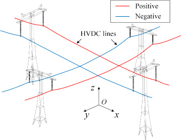
Structure diagram of the cross-over HVDC lines.

2. Methodology of ion flow field calculation

2.1. Basic equations

The diagram of cross-over two circuit UHVDC transmission lines is shown in Fig. 1. Because of the high electric field strength, the air near the lines will be ionized, and the ions will drift to the ground or the transmission lines with opposite polarity. The basis of electrostatic field calculation is to solve Poisson’s equation, as shown below $\begin{eqnarray}\displaystyle {\nabla}^{2}{\varphi}=-({\rho}_{+}-{\rho}_{-})/{\varepsilon}_{0} & & \displaystyle\end{eqnarray}$ (1) where 𝜑 is the electric potential, 𝜌 is the space charge density in the space, ϵ₀ is the dielectric constant in the air. Subscribe ‘+’ and ‘−’ represent positive and negative polarity, respectively.

The relationship between electric field vector E and electric potential 𝜑 is $\begin{eqnarray}\displaystyle \boldsymbol{E}=-{\nabla}{\varphi}. & & \displaystyle\end{eqnarray}$ (2) In (1), both 𝜑 and 𝜌 in are unknown. Thus, the ion transport equation, as shown in the following, is adopted to be the other governing equation. The relationship between space charge density 𝜌 and ion current density vector J is $\begin{eqnarray}\displaystyle \left\{\begin{array}{@{}l@{}}\boldsymbol{J}_{+}={\rho}_{+}K_{+}\boldsymbol{E}\\[6.0pt] \boldsymbol{J}_{-}=-{\rho}_{-}K_{-}\boldsymbol{E}\end{array}\right. & & \displaystyle\end{eqnarray}$ (3) where K is the ion mobility rate. This equation can be written as a convection dominated partial differential equation about space charge density 𝜌₊ and 𝜌₋ $\begin{eqnarray}\displaystyle \left\{\begin{array}{@{}l@{}}{\nabla}{\varphi}\cdot {\nabla}{\rho}_{+}={\displaystyle \frac{{\rho}_{+}^{2}}{{\varepsilon}_{0}}}-\left({\displaystyle \frac{1}{{\varepsilon}_{0}}}-{\displaystyle \frac{R}{eK_{+}}}\right){\rho}_{-}{\rho}_{+}\\[12.0pt] {\nabla}{\varphi}\cdot {\nabla}{\rho}_{-}=-{\displaystyle \frac{{\rho}_{-}^{2}}{{\varepsilon}_{0}}}+\left({\displaystyle \frac{1}{{\varepsilon}_{0}}}-{\displaystyle \frac{R}{eK_{-}}}\right){\rho}_{-}{\rho}_{+}\end{array}\right. & & \displaystyle\end{eqnarray}$ (4) where R is the ion recombination coefficient, e is the charge of the electron. The unique solutions of 𝜑 and 𝜌 are obtained by solving the coupled Eqs (1) and (4). In this paper, the calculation domain is meshed by first-order tetrahedron elements. The initial values of 𝜌₊ and 𝜌₋ are set on the corona conductor surfaces at first. Then, the variable 𝜑 in Poisson’s equation is solved by 3D FEM. In the next, 𝜌₊ and 𝜌₋ in the space are solved by upstream differential method from the upstream boundaries, i.e., the surface of positive and negative transmission lines, respectively. Finally, ion densities on corona conductor surfaces are corrected by previous calculated results, and the calculating procedure of 𝜑 and 𝜌 will be repeated until the solution is convergent.

2.2. Correction of space charge density

The boundary conditions are of vital importance when solving the governing equations. The electric potentials 𝜑 on the conductor surfaces are the applied voltages, and potential on the ground is zero. Therefore, the boundary conditions for Poisson’s equation are sufficient. However, the boundary conditions of first-order ion transport equation, in other words, space charge densities on the conductor surfaces, are unknown. Not only the low calculating accuracy but also the non-convergence issues will be caused if the boundary condition is inappropriate.

Kaptzov’s assumption is widely used to identify the validity of the boundary condition of ion transport equation. This assumption claims the electric field on the conductor surface remains constant at the corona onset value after the corona has been stable. In the most common situation, there is only one circuit line in the space, and the ion flow field is calculated by 2D method. Besides, the most concerned physical characteristic is the ion flow field on the ground. Accordingly, the space charge density distribution can be considered as uniform [9,10,16]. The value of space charge density is determined by a predictor-corrector process. At the n-th iteration, the space charge density on the conductor surface is corrected by: $\begin{eqnarray}\displaystyle {\rho}_{\text{2D}}(n)={\rho}_{\text{2D}}(n-1)\left(1+\frac{E_{\max }(n)-E_{\text{on}}}{E_{\max }(n)+E_{\text{on}}}\right) & & \displaystyle\end{eqnarray}$ (5) where 𝜌_2D and E _max are the space charge density and maximum electric field on the conductor surface in 2D calculation, respectively. Equation (5) is named as “uniform assumption” in the following.

In order to improve the calculating accuracy of 3D problems or bundle transmission lines, an assumption of conductor surface ion distribution in linear form is then adopted [14–16]: $\begin{eqnarray}\displaystyle {\rho}_{\text{3D}}={\rho}_{\text{2D}}\frac{E_{\text{nom, 3D}}-E_{\text{on}}}{E_{\text{nom, 2D}}-E_{\text{on}}} & & \displaystyle\end{eqnarray}$ (6) where E _nom, 2D and E _nom, 3D are the nominal electric fields on the conductor surface, i.e., electric fields without ions in 2D situation and 3D crossing situation, respectively. 𝜌_3D is the space charge density on the crossing conductor surface. Equation (6) is named as “linear assumption”. In ref. [14], the linear assumption is proved to be effective to deal with the crossing of HVAC and HVDC lines. The DC voltage is time-invariant. The influence of one circuit HVDC line on the corona of the other circuit HVDC line is much greater compared with HVAC lines. Therefore, the space charge density distribution on the crossing HVDC conductor surfaces will be more complex. In addition, higher calculation accuracy is required to study the electric field in the space near the lines. An additional treatment to correct the space charge density on the crossing conductor surface point by point is applied: $\begin{eqnarray}\displaystyle {\rho}_{3\text{D, }i}(n)={\rho}_{3\text{D, }i}(n-1)\left(1+{\mu}\frac{E_{i}(n)-E_{\text{on}}}{E_{i}(n)+E_{\text{on}}}\right) & & \displaystyle\end{eqnarray}$ (7) where subscript i is the i-th node on the corona conductor surface, 𝜌_3D, i is the space charge density on node i, E _i is the electric field on node i. 𝜇 is a factor to control the convergence speed. In this paper, 𝜇 = 1.0. Equation (7) is named as “correcting point by point”. The aim of using (7) is to assure the electric field on each node of conductor surfaces satisfying Kaptzov’s assumption.

Fig. 2.

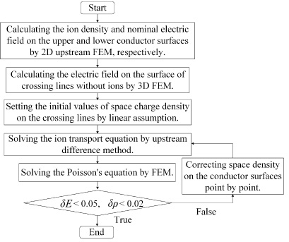
The flowchart of 3D upstream FEM.

In order to improve the calculation efficiency and convergence, the calculated results of (6) should be used as the initial value of (7) In addition (6) is based on the results of (5). The flow chart of the 3D upstream FEM calculation with optimized surface space charge density treatment is presented in Fig. 2. 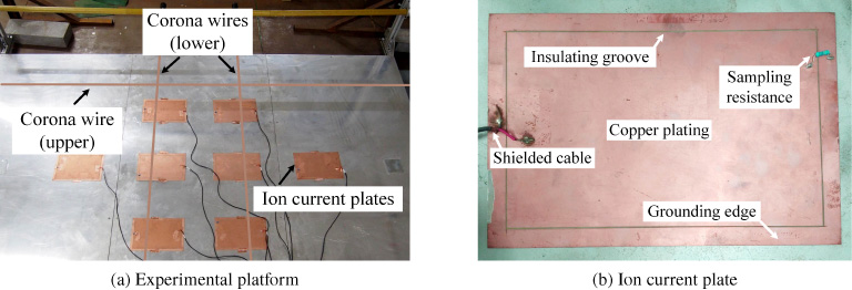Considering the numerical calculation error generated by 3D FEM modeling, the convergence conditions in the ion flow field calculation are defined as: $\begin{eqnarray}\displaystyle \text{} & \text{} & \displaystyle {\delta}E=\max \left|\displaystyle \frac{E_{i}-E_{\text{on}}}{E_{\text{on}}}\right|<0.05\end{eqnarray}$ (8) $\begin{eqnarray}\displaystyle \text{} & \text{} & \displaystyle {\delta}{\rho}=\left|\displaystyle \frac{{\rho}_{\max }(n)-{\rho}_{\max }(n-1)}{{\rho}_{\max }(n)}\right|<0.02\end{eqnarray}$ (9) where δE and δ𝜌 are the convergence criterions of electric field and space charge density. 𝜌_max(n) is the maximum space charge density in the whole calculation domain in n-th iteration.

3. Experiments

The experimental platform including different polarities and cross-over structures of corona wires is presented in Fig. 3(a). The upper and lower circuits HVDC corona wires are crossing with the angle of 90°. A sensor array composed of eight ion current plates are arranged on the ground. The composition of ion current plate is shown in Fig. 3(b). The ions that flow to the inner copper plating will pass through the sampling resistance. The voltage on the resistance is recorded by the data acquisition system, and the value of ion current density J is calculated by Ohm’s law.

Comparison between measured and calculated results are listed in Table 1. The ground-level ion current densities vary widely in different positions. In the experiment, the maximum difference between measured and calculated values at all positions is 0.75 μA∕m², which is 7.4% of the measured results. The agreement of measured and calculated results indicates the calculation method is able to satisfy the engineering demand.

Fig. 3.

Measurement of ground-level ion current density.

Table 1

Comparison of measured and calculated results

	Crossing of +60 kV and ±45 kV wires			Crossing of −60 kV and ±45 kV wires
Position	Measurement	Calculation	Error	Measurement	Calculation	Error
(m)	(μA∕m²)	(μA∕m² )	(μA∕m² )	(μA∕m² )	(μA∕m² )	(μA∕m² )
(−0.25,0.45)	0.62	0.67	−0.05	7.27	6.64	0.63
(0.25, 0.45)	−11.20	−10.53	−0.67	−5.19	−4.96	−0.23
(−0.75,0)	2.27	2.04	0.23	−0.90	−1.13	0.23
(−0.25,0)	0.14	0.21	−0.07	2.92	2.71	0.21
(0.25, 0)	−10.02	−10.77	0.75	0.04	0.07	−0.03
(0.75, 0)	1.05	1.21	−0.16	−1.67	−1.54	−0.13
(−0.25, −0.45)	0.64	0.67	−0.03	6.32	6.64	−0.32
(0.25, −0.45)	−10.86	−10.53	−0.33	−4.55	−4.96	0.41

4. Calculation of the crossing ±800 kV HVDC lines

Electric field strength and space charge density near the crossing two circuit ±800 kV UHVDC lines are calculated based on the method above. The structure of crossing lines is shown in Fig. 4. The height of upper and lower circuit lines is 30 m and 18 m, respectively. The polar distances are 22 m. Each bundle line has 6 sub-conductors. The area of intersecting surface of every sub-conductor is 720 mm². To reduce the calculating cost, the bundle conductors are simplified to equivalent single conductor [13].

The length of lines in 3D calculation is 100 m. In the FEM model, 488703 nodes and 2756154 elements are generated. The calculating results with the three kinds of surface ion correcting treatments, i.e., the uniform assumption (5), linear assumption (6) and correcting point by point (7), are analyzed. On the surface of lower positive conductor (x = 11 m, z = 18.345 m), the calculated electric field distributions are presented in Fig. 5.

In Fig. 5, the corona onset electric field is used as the reference value. According to Kaptzov’s assumption, the electric field on the corona conductor surface should equal to 1 p.u. If the surface electric field is less than 1 p.u., the applied value of space charge boundary condition is too larger. By contrast, if the electric field is more than 1 p.u., the boundary condition of ion transport equation is too small. These errors will inevitablely influence the calculated ion flow field. When using uniform assumption and linear assumption, the relative errors of electric field on conductor surfaces are 43.3% and 34.2%, respectively. When the space charge density boundary condition is corrected point by point, the relative error is reduced to 4.9%. To correct space charge density point by point is able to assure the satisfaction of Kaptzov’s assumption.

Fig. 4.

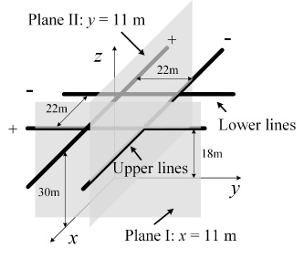
Calculation planes in the space.

Fig. 5.

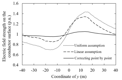
Comparison of space charge density treatments on the conductor surface.

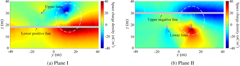
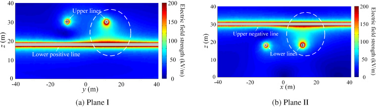
4.1. Ion flow field distribution in the space

Two calculation planes (Plane I: x = 11 m, Plane II: y = 11 m) are selected to present the distribution of space charges and electric field, as showed in Fig. 4. Calculated space charges and electric fields are shown in Fig. 6 and Fig. 7, respectively.

In Fig. 6, it can be seen that the corona discharge in the opposite polar crossing area is significantly enhanced. The corona enhanced areas are highlighted by the white circles. At the same voltage level, the corona onset electric field of negative polarity is always lower the positive polarity, and more negative space charges should be generated. However, Fig. 6(b) indicates the space charge density around lower positive line is much larger than the negative line. Compared with there is only one circuit line in the space, the maximum space charge density on the surface of upper negative line in Plane I increases 45.2%. On the lower positive line in Plane II, the maximum value of space charge density increases 57.6%.

Figure 7 presents the electric field amplitude in the space. Because of the constraint of Kaptzov’s assumption, the electric fields on the conductor surfaces remain at the corona onset electric field. But the electric field strength in the opposite polarity crossing area, as is shown in the white circles, is much higher than the same polarity. Therefore, the crossing structure should be checked in order to keep enough long insulating distance between positive and negative polarities.

Fig. 6.

Space charge distribution.

Fig. 7.

Electric field distribution.

5. Conclusion

Ion flow field near the cross-over two circuit UHVDC lines is studied by using 3D upstream FEM. The space charge density correcting treatment on the conductor surface is adopted to improve the calculating accuracy. Reduced-scale experiments with crossing HVDC corona wires are carried out in the laboratory. The ground-level ion current density distribution is measured by the ion current plate array, and the calculation method is verified by the measured results.

Based on the calculation, electric field and space charge density near the crossing two circuit ±800 kV UHVDC lines are analyzed. In the area where the polarity of upper and lower conductor is opposite, the corona discharge level is stronger, and the electric field is larger. More attention should be given when designing the crossing of opposite polarities in the engineering practice.

Footnotes

Acknowledgements

This work was supported by the National Nature Science Foundation of China under Grant 51577064 and Science and Technology Project of State Grid Corporation of China GYB17201400185.

References

Maruvada

P.S.

, Electric field and ion current environment of HVDC transmission lines: Comparison of calculations and measurements, IEEE Trans. Power Deli. 27 (2012), 401–410.

Ueli

and Franck

C.M.

, Ion-flow field calculations of AC/DC hybrid transmission lines, IEEE Trans. Power Deli. 28 (2013), 294–302.

Maruvada

P.S.

, Influence of ambient electric field on the corona performance of HVdc transmission lines, IEEE Trans. Power Deli. 29 (2014), 691–698.

Thomas

Pfeiffer

and Franck

C.M.

, Improved coupled ion-flow field calculation method for AC/DC hybrid overhead power lines, IEEE Trans. Power Deli. 29 (2014), 2493–2501.

Luo

Cui

Zhang

and Lu

, Calculation of the 3D ionized field under HVDC transmission lines, IEEE Trans. Magn. 47 (2011), 1406–1409.

Qiao

Zou

and Li

, Calculation of the ionised field and the corona losses of high-voltage direct current transmission lines using a finite-difference-based flux tracing method, IET Gene., Trans. & Distrib. 9 (2015), 348–357.

Wang

Chen

and Li

, 3-D electric field computation of steeple rooftop houses near HVDC transmission lines, IEEE Trans. Magn. 53 (2017), 7205704.

Xiao

Zhang

and He

, Calculation of 3-D ion flow field at the crossing of HVDC transmission lines by method of characteristics, IEEE Trans. Power Deli. 33 (2017), 1611–1619, doi:10.1109/TPWRD.2017.2737006.

Janischewskyj

and Cela

, Finite element solution for electric fields of coronating DC transmission lines, IEEE Trans. Power App. Syst. PAS-98 (1979), 1000–1012.

10.

Takuma

and Kawamoto

, A very stable calculation method for ion flow field of HVDC transmission lines, IEEE Trans. Power Deli. 2 (1987), 189–198.

11.

Zhen

Cui

Fang

and Zhou

, 3D finite-element method for calculating the ionized field and the ion current of the human body model under the UHVDC lines, IEEE Trans. Power Deli. 28 (2013), 965–971.

12.

Huang

Ruan

Liao

Jin

and Wang

, Improved 3D upwind FEM for solving ionized field of HVDC transmission lines, Proc. CSEE 33 (2013), 152–159.

13.

Zhou

Cui

Liu

and Li

, Simulation of ion-flow field at the crossing of HVDC and HVAC transmission lines, IEEE Trans. Power Deli. 27 (2012), 2382–2389.

14.

Zhang

Zeng

and Wang

, Calculation of the ion flow field of AC-DC hybrid transmission lines, IET Gener. Trans. & Distrib. 3 (2009), 911–918.

15.

Zhou

Cui

Fang

and Zhen

, Spatial distribution of ion current around HVDC bundle conductors, IEEE Trans. Power Deli. 27 (2012), 380–390.

16.

Wang

Chen

and Xie

, Influence of space charge distribution around the conductor surface on ionized field computation, in: IEEE PES Asia Pacific Power and Energy Engineering Conference (APPEEC), Xi'an, China, 2016, pp. 687–691.