A new quantitative non-destructive testing approach of broken wires for steel wire rope

Abstract

In order to solve the problems including poor signal denoising effect, low recognition rate, and poor real-time performance in wire rope magnetic flux leakage (MFL) testing, this paper proposes a new algorithm combining kernel extreme learning machine (KELM) with compressed sensing wavelet (CSW). Firstly, we consider a new mechanism and regularized orthogonal matching pursuit (ROMP) into CSW, and combine double-density wavelet transform (DD-DWT) to improve the result of wire rope signal noise reduction; Then, an effective normalization method is developed to improve the accuracy of classification. Finally, the detection accuracy and efficiency in wire rope quantitative identification are ameliorated through KELM. The effectiveness and novelties of the proposed algorithms are verified by the experimental platform based on unsaturated magnetic excitation non-destructive testing (NDT) device.

Keywords

Wire rope non-destructive testing compressed sensing kernel extreme learning machine quantitative identification

1. Introduction

As a key component of engineering load, wire ropes are widely employed in many fields of national economic construction, such as mines, freight ropeways, suspension bridges, buildings, and ports [1]. It is noteworthy that long-term harsh and uncertain working conditions may result in wire rope damage: reduced cross-sectional area of metal due to wear and corrosion, broken wires due to fatigue and surface hardening, changes in internal properties and deformation of wire ropes [2–6]. With the accumulation of daily use, the reduction of wire rope strength will seriously affect the normal operation of industrial production and personnel safety. Therefore, wire rope damage detection is worth exploring.

In general, wire rope damages can be divided into local defects and metal cross-sectional area lossing according to the nature and characteristics of wire rope damage [3–5]. Accordingly, electromagnetic detection and ultrasonic detection are widely used for wire rope damage detection and there also exist other damage testing methods including X-ray testing, acoustic emission testing, and eddy current testing [6]. For example, Yan et al. [7] employed a three-dimensional finite element method (FEM) to analyze the MFL signals, which provided theoretical guidance for detection signal analysis and hardware design. Zhao et al. [8] established a wire rope leakage magnetic detection platform, and obtained the two-dimensional MFL signal of the wire rope defect by analyzing the influence of defect parameters on the leakage magnetic field distribution. In [9–11], the researchers realized wire rope inspection via testing characteristics of the MFL signal at the wire rope defect. To investigate the effects of ultrasonic guided waves (UGW) propagation, Raisutis [12] applied 3D FEM for simulating the two types of the acoustic contact between neighboring wires, in which the simulation results showed that, even in the case of the slip contact between wires, the UGW can also be used for integrity analysis wire ropes and to detect the defective ones. Du [13] investigated and established finite element model of the steel wire rope; through simulating the finite element model of different broken wires, the influence of the number of broken wires on the safety factor can be studied. Other detection methods have not been fully applied to wire rope inspection; as we know, Ma et al. [14] performed a torsion test on steel wire based on the magnetic memory method; the research demonstrates that magnetic memory technique is an effective method for determining early damage of steel wire under torsion and can provide certain reference for quantitative analysis of the relationship between damage and signals. Feng and Kang [15] explored how eddy currents affect MFL signals in high-speed testing, which provides a theoretical reference for wire rope eddy current testing.

In the test system, the design of the hardware is also crucial, which can affect the quality of the MFL signal. Yan and Zhang [7] presented a simplified magnetic circuit with two half-sized radial magnetizing ring NdFeB magnets to excite the fine steel wire rope. The fine steel wire rope NDT system not only had simple and lightweight excitation structure, but also had a stable performance power system and a signal processing circuit that can enhance the signal-to-noise ratio (SNR) of the defect MFL signal. Thus, the system realized on-line testing in an environment with strong electromagnetic interference. Cao [16] obtained the defect data from a detection device based on a printed circuit board split differential coil. The device was useful for a certain span in the axial direction of the wire rope, but it was not sensitive to small width defects and circumferential defect information [17]. Yan and Zhang [18] proposed an iron core, which is used for coil winding skeleton, for wire rope NDT using inductive coil; this simplified structure improved the SNR of the coil output signal and reduces the influence of the lift-off distance between coil and wire rope on the detection result.

The MFL signals collected by magnetic sensors contain various noises. To get pure defect information, it is necessary to filter system’s noises. H.Y. Wang et al. [19] proposed an adaptive wavelet threshold denoising method [20] based on a new threshold function, which can effectively inhibit the effect of noise on the MFL signal of the wire rope. J. Zhang and X. Tan [11] utilized the wavelet based on compressed sensing [21] to denoise the strand wave, but compressed sensing restored a lot of noises [17]; then [10] combined the Hilbert-Huang transform (HHT) [22] and compressed sensing wavelet filtering (CSWF) [23] to reduce the various background noises. D. Zhang et al. [24] designed a spatial filter to suppress the strand texture of defects of grayscale image. Zhang and Zheng [17] employed a wavelet filter algorithm [25,26] based on ensemble empirical mode decomposition (EEMD) [27] for reducing the system noise and improved the resolution of defect grayscale by adopting the wavelet super-resolution reconstruction technique [17,28]. Y.N. Qin et al. [29] used wavelet decomposition and reconstruction [26] to eliminate the background noise of the original signal of corrosion failure adequately, and took the support vector machine (SVM) [30] with a radial basis function classified to conduct the fault pattern recognition. Z. Wan et al. [31] investigated the theory on optimal wavelet packet with the least squares support vector machine (LS-SVM) [32] to diagnose elevator faults, which was then validated by the experiment. Taking into account the previously mentioned wire rope classification methods, back propagation (BP) neural networks [33] have been used by a number of researchers [11,17,24,34]. However, BP neural networks have the disadvantages of poor generalization and slow convergence.

The common filtering algorithms cannot fully filter out the noise; conventional recognition algorithms [10,11,30,32] are easy to fall into local minimum and have long time for training and testing; traditional electromagnetic NDT devices suffer from some shortcomings, such as large and heavy, low sensitivity, and inconvenience. Through the implementation of CSW algorithm which combines constraint setting with ROMP [35] and DD-DWT [36], the noises of wire ropes MFL were suppressed effectively. To achieve the quantitative identification of broken wires, the defects were located and segmented by the modulus maxima method. The new normalization rule was proposed to normalize data. The MFL grayscale images were obtained from normalizing data [11,17], which was the input of KELM neural network [37,38]. By using KELM as the recognition algorithm [39], the classification speed and accuracy had been improved. To overcome the limitations of existing detection devices, we utilize a detection device based on unsaturated magnetic excitation, with giant magneto-resistance (GMR) sensors for excitation signal acquisition [17].

2. Data collection

The adopted data acquisition device in this study, as shown in Fig. 1, includes unsaturated magnetic excitation source, sensor array, pulse generation and data acquisition unit, data storage, and control system.

Fig. 1.

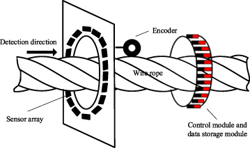
Schematic of data acquisition device.

The excitation device consists of a plurality of strip permanent magnets uniformly distributed around the wire rope circumference. The sensor array adopts 18 GMR sensors, which are distributed on the rope circumferential direction to collect magnetic data. The acquisition system uses pulses provided by a grating encoder to ensure equal-space sampling. The acquired MFL data is stored on the SD card, and the control system uses an STM32F407 chip to control the whole data acquisition system.

The specific collection processes of remanence detection are as follows: The wire rope is loaded with unsaturated excitation field, the photoelectric encoder generates spatially equidistant pulses and send them to control system when the acquisition system move along the axial direction of the wire rope. According to the encoder pulse signal, the control board collects the data from 18 channels. Then, the acquired data is stored on the SD card after analog-digital (AD) conversion and differential amplification. Through baseline elimination and other denoising operations, the defect information could be obvious.

A two-dimensional array of M × N of wire rope information resolution is obtained by unfolding the data along circumferential direction, where M is the number of sensors (here, the number is 18) and the N depends on the number of pulses. Figure 2 shows parts of the expanded raw data.

Fig. 2.

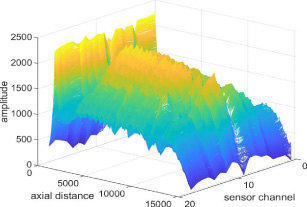
Schematic of original data.

3. Data processing

The raw data from collection system contains various sources of noise, including high-frequency MFL noise, non-uniformity of magnetization, strand wave noise produced by helix structure of wire rope, and the noise caused by lift-off distance. It is obvious that the aforementioned noise interference makes it difficult to locate and classify the damage. Therefore, inhibiting the noise of original data is necessary. In this section, we will utilize wavelet analysis and DD-DWT to eliminate the baseline noise and high frequency noise. Then we adopt the proposed CSW algorithm to remove strand wave and other noise.

3.1. Signal pre-processing

The original signal from GMR sensor array should be pre-processed, which is to suppress noise from high-frequency magnetic leakage and baseline noise caused by channel imbalance. DD-DWT and wavelet analysis can implement signal preprocessing by denoising.

Wavelet basis functions are orthogonal, thus, wavelet analysis has the characteristics of multiresolution analysis [11]. And it can be successfully applied to nonlinear and non-stationary systems because wavelet analysis can extract the required information from the data. A one-dimensional signal can be decomposed to different frequency and scale sequences by wavelet transform. Hence, by using wavelet transform to decompose and reconstruct the signal, the raw signal can be clearer. $\begin{eqnarray}\displaystyle & \displaystyle \left\{\begin{array}{@{}l@{}}a_{j+1}(k)=\displaystyle \mathop{\sum }_{n=-\infty }^{\infty }a_{j}(n)h_{0}(n-2k)=a_{j}(k)\times \bar{h}_{0}(2k)\\[14.0pt] d_{j+1}(k)=\displaystyle \mathop{\sum }_{n=-\infty }^{\infty }a_{j}(n)h_{1}(n-2k)=a_{j}(k)\times \bar{h}_{1}(2k)\\ \end{array}\right. & \displaystyle\end{eqnarray}$ (1) $\begin{eqnarray}\displaystyle & \displaystyle a_{j}(k)=\mathop{\sum }_{n=-\infty }^{\infty }a_{(j+1)}(n)h_{0}(k-2n)+\mathop{\sum }_{n=-\infty }^{\infty }d_{(j+1)}(n)h_{1}(k-2n) & \displaystyle\end{eqnarray}$ (2) where h ₀ is a low-pass filter and h ₁ is a high-pass filter. The details of using wavelet to remove the baseline is given as follows: Db4 wavelet is selected to decompose the signal into 7 layers with Eq. (1), the baseline of signal is located in the low frequency band and the high frequency coefficient contains few defect information, so the signal reconstructed with Eq. (2) can eliminate the baseline and part of the high frequency noise by setting the coefficients of the first and last layer to zero. Figure 3(a) and Fig. 3(b) show the raw signal and baseline removal signal of single- channel, respectively.

Fig. 3.

Single-channel signal.

The DD-DWT has double sampling frequency of common wavelet and it is approximately shift-invariant. In the DD-DWT, the single lowpass and two highpass filters constitute a three-channel perfect reconstruction filter bank. The double-density DWT is based on a single scaling function and two distinct wavelets [36], where the two wavelets and scaling function are shown as follows: $\begin{eqnarray}\displaystyle & \displaystyle {\varphi}(t)=\sqrt{2}\mathop{\sum }_{n}h_{0}(n){\varphi}(2t-n) & \displaystyle\end{eqnarray}$ (3) $\begin{eqnarray}\displaystyle & \displaystyle {\phi}_{i}(t)=\sqrt{2}\mathop{\sum }_{n}h_{i}(n){\varphi}(2t-n),\quad i=1,2 & \displaystyle\end{eqnarray}$ (4) $\begin{eqnarray}\displaystyle & \displaystyle {\phi}_{1}(t)={\phi}_{2}(t-0.5). & \displaystyle\end{eqnarray}$ (5) The double-density wavelet is employed to remove the high frequency noise: every array signal uses double-density wavelet to decompose, with available lowest coefficients retained and the rest ones set to zero. Figure 4 shows that the MFL signal has been pre-processed. Figure 5 shows the image of defects that has been pre-processed.

Fig. 4.

Pre-processed single-channel signal.

Fig. 5.

Image of pre-processed signal (the raw data is obtained from Fig. 2).

From Fig. 3(a) and Fig. 4, it is obvious that the flaws signal is clearer. With the comparison of Fig. 2 and Fig. 5, it shows that the preprocessed method removes baseline and high frequency noise.

3.2. Signal re-processing

After removing the signal baseline drift and high-frequency noise, the signal also contains a large amount of strand waves and other noise. In this section, we propose the CSW algorithm which contains a constraint and ROMP to inhibit the strand waves. By comparing the common CS algorithms with our proposed CSW, it will be proved that our algorithm is the most effective method.

The collected wire rope defect information contains sensor information of 18 channels, but the defect information does not exist in all channels. CS is used in each channel, thus, some of the noise would be restored inevitably. In order to reduce noise more and improve SNR, we consider that we could only find the channels including flaws information and apply CS to reconstruct the signal; ROMP has not only the speed and ease of implementation of the greedy methods but also has strong stability which makes the recovery of approximately sparse signals accurate [35], therefore, we adopted ROMP algorithm to reconstruct the sparse wavelet coefficients. The core of ROMP algorithm is to find the n columns that best match the current residual error. After obtaining the reconstructed vector from the least squares, the residue is update and repeat iteration until K.

Fig. 6.

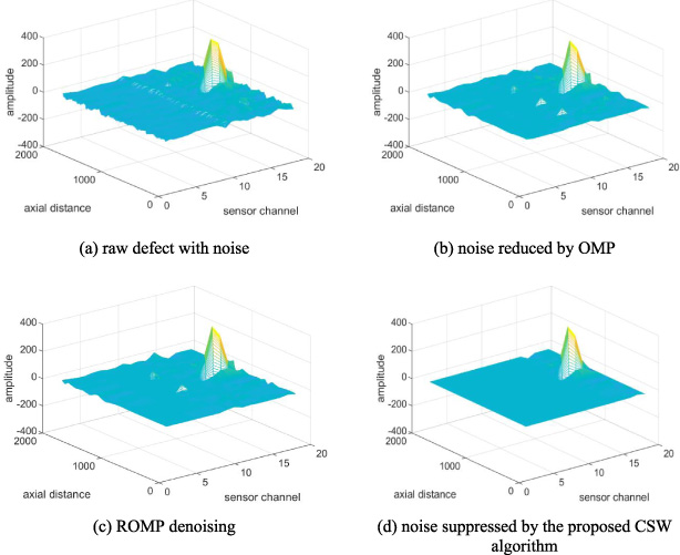
Image of a defect signal.

The proposed CSW algorithm is listed as follows:

f _r(i) = f _d(i) + f _n(i), i = 1 ∼18, where f _r is the raw data, f _d is the defect information, f _n is noise, and i is the number of channel; select maximum and minimum peaks of the signal: min(i) = peak[−f _r(i)] and max(i) = peak[f _r(i)], if max(i) > 50 and min(i) > 50, x = f _r(i), or f _r(i) = 0.

The pre-processed signal x is decomposed by Mallat algorithm [25,26], and the wavelet coefficients W _j under different scales are obtained.

Select the appropriate random measurement matrix 𝜙, and calculate the wavelet coefficients of linear measurement Y _j under Y _j = 𝜙W _j.

Through the ROMP algorithm, the most-sparse wavelet coefficient is reconstructed [11]; the algorithm steps are as follows:

Initialize residue 𝛾₀ = y, index set A _t = 𝜑 (empty set), iteration t = 1;

The absolute value of the inner product of the residuals and the measurement matrix is calculated u = abs[〈𝛾₀, 𝜑_j〉], j = 1 ∼ N. The n columns with the largest absolute value of the inner product are obtained, then a set J containing serial number j of the corresponding measurement matrix is constituted.

The set of column vector ordinals, J ₀, satisfies |u (i) ≤ 2|u (j)||, for i, j ∈ J ₀, and ∑ _j|u (j)|² is maximum, for j ∈ J ₀. The subscript A _t = A _t−1 ∪ J ₀ and the most orthogonal column of 𝜑𝜑_t = 𝜑_t−1 ∪𝜑_J
₀ are stored.

The least-squares method is used to calculate $w_{t}=argmin||y-{\varphi}_{t}w_{t}||_{2}=({\varphi}_{t}^{H}{\varphi}_{t})^{-1}{\varphi}_{t}^{H}y$ .

The residue, $r_{t}=y-y_{t}={\varphi}_{t}w_{t}={\varphi}_{t}({\varphi}_{t}^{H}{\varphi}_{t})^{-1}{\varphi}_{t}^{H}y$ , is updated; t = t +1, if t ≤ K (t is 1 to K, K is the sparse degree; here is 3), return to II, otherwise stop the iteration.

The clear signal can be reestablished through using approximate wavelet coefficients from CSW.

Figure 6(a) shows the preprocessed image, and it has damage data with strand wave and other noise. CS with OMP, CS with ROMP and the proposed CSW are adopted to reduce the noise. The results are shown in Fig. 6. Figure 6(b) is the image processed by OMP, the image processed by ROMP is displayed in Fig. 6(c), and the image with noise suppressed by the proposed CSW algorithm is shown in Fig. 6(d).

The comparison of denoising results in Fig. 6 clearly indicates that the proposed CSW algorithm fully suppresses the strand wave and noise. It reduces noise recovery and reaches better effect than common CS for wire rope noise reduction and the image denoised by CSW has higher SNR. That makes contribution to the subsequent processing.

To describe the effect of denoising effect, we define the SNR as $\text{SNR}=10\text{Lg}\left(20\frac{A_{s}}{A_{n}}\right)$ , where A _s is the area between the defect signal and x axial and A _n is the area between the noise and x axial. We have applied several denoising methods to MFL data: OMP algorithm [11], ROMP algorithm, and our proposed algorithm. We randomly select 10 groups signals and Table 1 shows the SNR calculated for each method. Our proposed algorithm has better results when denoising the signal of defect.

Table 1

SNR of several denoising algorithms

Group	Raw signal (dB)	OMP algorithm (dB)	ROMP algorithm (dB)	Proposed algorithm (dB)
1	22.893	28.897	29.406	30.525
2	20.799	25.628	26.027	27.741
3	23.286	28.88	29.852	38.01
4	21.582	26.676	26.797	37.727
5	30.510	39.288	38.630	39.727
6	24.377	31.382	32.539	33.878
7	20.360	25.065	25.501	26.319
8	22.957	29.214	29.549	34.217
9	27.057	36.155	36.585	36.573
10	23.437	29.281	29.778	35.391

4. Image processing

The image expression is intuitive and concise, therefore, we employ mature image processing method for defects treatment. In this section, we get the obvious damage image by defect location and segmentation, gray normalization, and three spline interpolations, which make preparation for the quantitative identification of wire rope.

4.1. Defect location and segmentation

The local modulus maxima algorithm is applied to locate the defects: the circumference data is added up to search for the data location with the largest modulus, then the position is considered as the axial center of the damage, with 149 interception data to the left and 150 points to the right; the location of maximum value of one-dimensional data obtained by axial summation of the MFL signal is used for judging whether the part is the center of the defect. If not, the cut and mend method is used to make it at the center position. A defect image with 300 × 18 pixels is obtained from procedure steps and the resolution will be promoted in next section.

4.2. Defect image visualization

The min-max normalization refers to x ^∗ = (x − min)∕(max−min), but it does not work very well in this study. Since it is impossible to guarantee that every wire rope is exactly the same during the excitation process, it makes difficulty to distinguish the number of broken wires as shown in Fig. 7(a) if the data is normalized using min-max normalization method. In order to solve the problem and visualize the defects with a unified standard, the pure defects are stretched between 0–255 with a same scale. The proposed rule normalization is presented as formula (6). $\begin{eqnarray}\displaystyle \mathit{IM}_{N}(j,q)=255\times \left(\frac{\mathit{IM}(j,q)}{700}+0.5\right) & & \displaystyle\end{eqnarray}$ (6) where IM _N is the normalized image, IM is raw image, and j, q represent 300 and 18 that is the current pixel of a defect image.

Fig. 7.

The gray images with 7 broken wires.

Figure 7(a) shows that defect grayscale images of the same defects vary widely by min-max normalization: the size and gray distribution of defects are very different. It can result in a great obstacle for the quantitative identification of defects in the next section. Figure 7(b) shows images with the proposed regulation to normalize seven broken wires. While, the images with the same broken wires have little difference by using the proposed normalized method.

The normalized damage is shown in Fig. 8. The MFL data captured by the 18 sensors with high sensitivity around the wire ropes has low circumferential resolution. Three spline interpolations are performed to enhance the circumferential resolution of the clear signals to 300 × 300 pixels. Figure 9 shows the image after circumferential interpolation.

Fig. 8.

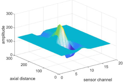
Schematic of normalized defect.

Fig. 9.

Schematic of a defect after interpolation.

Figure 10 shows the grayscale of the six defects that contains one, two, three, four, five, and seven broken wires.

Fig. 10.

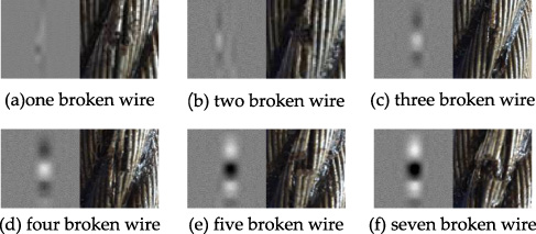
Image of broken wires.

5. Quantitative recognition

In this section, a KELM neural network is used to classify the defect. Due to kernel functions existing, the running speed is faster. KELM is proved as the most effective recognition method obtained by the comparison of four different classification methods: nearest neighbor (NN), least-square support vector machine (LSSVM), extreme learning machine (ELM), and kernel extreme learning machine (KELM) [39].

5.1. Kernel Extreme Learning Machine (KELM)

Extreme learning machine (ELM) is a single-layer feedforward neural network classifier, which is well-known in many different applications [40]. Traditionally, a gradient-based method such as back-propagation (BP) algorithm suffers from local minima and learning rate. ELM does not need to re-adjust parameters for its hidden layers and it has random projection of hidden layer with random input weights [38,39]. The goal of ELM is to minimize both the training errors and the norm of output weight at the same time [38]. ELM has numerous significant advantages such as improved generalization, learning speed, ease of implementation, and minimal human intervention [39].

KELM is an intelligent learning algorithm with strong nonlinear fitting ability, which is an improvement on ELM. The random input weights and bias in KELM can be avoided and KELM is formulated by applying Mercer condition [41] to ELM [39]. Namely, KELM has greater generalization and stability than ELM.

The principle of KELM for classification can be described as follows [39,40]:

Given a set of samples X = [x ₁, x ₂, …, x _N] ∈ R ^d×N with label T = [t ₁, t ₂, …, t _N] ∈ R ^c×N, where N is the number of sample, d is the dimension of sample, and c is the number of classes. If x _i(i = 1, …, N) belongs to the k-th class, the k-th position of t _i(i = 1, …, N) is set as 1, and 0 otherwise. The hidden layer output matrix H with L hidden neurons is $\begin{eqnarray}\displaystyle H=\left[\begin{array}{@{}cccc@{}}h(w_{1}^{T}x_{1}+b_{1}) & h(w_{2}^{T}x_{1}+b_{2}) & \cdots ∼ & h(w_{L}^{T}x_{1}+b_{L})\\ \vdots & \vdots & \vdots & \vdots \\ h(w_{1}^{T}x_{N}+b_{1}) & h(w_{2}^{T}x_{N}+b_{2}) & \cdots ∼ & h(w_{L}^{T}x_{N}+b_{L})\end{array}\right] & & \displaystyle\end{eqnarray}$ (7) where h (⋅) is the activation function of hidden layer, W = [w ₁, w ₂, …, w _L] ∈ R ^d×L and B = [b ₁, b ₂, …, b _L]^T ∈ R ^L is the input weights and biases between randomly generated input layers and hidden layers, respectively. Hence, for ELM, it is to solve the following formula $\begin{eqnarray}\displaystyle \begin{array}{@{}l@{}}\displaystyle \text{}_{{\beta}\in R^{L\times C}}^{min}\Vert {\beta}\Vert ^{2}/2+\frac{C}{2}\mathop{\sum }_{i=1}^{N}\Vert {\xi}_{i}\Vert ^{2}\\[15.0pt] s.t.h(x_{i}){\beta}=t_{i}^{T}-{\xi}_{i}^{T},i=1\ldots N\Leftrightarrow H{\beta}=T^{T}-{\xi}^{T}\end{array} & & \displaystyle\end{eqnarray}$ (8) where 𝛽 ∈ R ^L×C indicates the output weight of hidden layer and output layer, 𝜉 = [𝜉₁, 𝜉₂, …, 𝜉_L] is the prediction error matrix of training data, and C is a penalty factor.

The solution of formula (8) is 𝛽^′ = H ⁺ T, where H ⁺ is the Moore-Penrose generalized inverse of H.

when N ≥ L, the output of the classifier can be computed as $\begin{eqnarray}\displaystyle y=h(z){\beta}^{\prime }=h(z)\left(H^{T}H+\frac{I_{L\times L}}{C}\right)^{-1}H^{T}T & & \displaystyle\end{eqnarray}$ (9) when N < L, the output of the classifier is obtained as $\begin{eqnarray}\displaystyle y=h(z){\beta}^{\prime }=h(z)H^{T}\left(H^{T}H+\frac{I_{L\times L}}{C}\right)^{-1}T. & & \displaystyle\end{eqnarray}$ (10)

In most cases, the number of neurons in the hidden layer is far less than the training samples. In ELM, the user usually knows the feature map. If a feature mapping is unknown to users, a kernel matrix for ELM can be defined: let 𝛺 = HH ^T ∈ R ^N×N, where 𝛺_{i, j} = h (x _i)h (x _j)^T = k (x _i, x _j) and k (⋅) is the kernel function. The output of KELM can be described as $\begin{eqnarray}\displaystyle y=h(z){\beta}^{\prime }=h(z)H^{T}\left(H^{T}H+\frac{I_{L\times L}}{C}\right)^{-1}T=\left[\begin{array}{@{}c@{}}k(z,x_{1})\\ \vdots \\ k(z,x_{N})\end{array}\right]^{T}\left({\Omega}+\frac{I_{N\times N}}{C}\right)^{-1}T. & & \displaystyle\end{eqnarray}$ (11)

5.2. Quantitative identification experiment

Steel wire ropes with a diameter of 28 mm and a structure of 6*36 are selected for the quantitative identification test. There are six kinds of broken wires, including 1, 2, 3, 4, 5 and 7 broken wires. 152 samples of various defects are selected in the experiment. 112 samples randomly selected are used as training samples, and the remaining 40 samples are used as test samples. Each defect image is arranged into a 1*90000 matrix as the input of artificial neural network, which do not require feature extraction. In this paper, a KELM network with 90000 ×112 ×6 is designed, where 90000 is the input nodes, 112 is the number of hidden layer nodes, and 6 is the output showing the type of defect. In addition, the type of kernel is RBF kernel. In this section, by comparing the accuracy of various identification methods including NN, LSSVM, ELM, and KELM for quantitative identification of wire rope defects, the most effective identification method is found.

We adjust the parameter of every method to get the best result. The parameters setting are as follows: the coefficients in LSSVM are automatically adjusted by using LSSVM-1.7 toolbox; In ELM, the penalty coefficient C is 900, the number L of hidden neurons is 1000, and the active function is ‘sig’; for KELM, the penalty coefficient and kernel parameter are set as 900 and 1000, respectively.

We conduct 20 experiments on each recognition network. The experimental results are shown in Table 2 and Table 3. In this paper, the allowable error is defined as the percentage of broken wires in the total wires.

Table 2
Recognition rate with 0.926% allowable error

Group NN LSSVM ELM KELM

1 95% 90% 87.5% 100%

2 80% 72.5% 67.5% 82.5%

3 87.5% 80% 70% 87.5%

4 97.5% 85% 80% 97.5%

5 90% 77.5% 80% 90%

6 90% 82.5% 82.5% 95%

7 97.5% 77.5% 77.5% 97.5%

8 87.5% 80% 77.5% 87.5%

9 92.5% 90% 90% 97.5%

10 92.5% 90% 90% 97.5%

11 100% 82.5% 82.5% 100%

12 85% 70% 85% 87.5%

13 90% 67.5% 80% 90%

14 97.5% 90% 85% 95%

15 87.5% 87.5% 77.5% 90%

16 90% 90% 85% 90%

17 97.5% 97.5% 90% 95%

18 95% 95% 82.5% 95%

19 95% 95% 90% 90%

20 90% 90% 87.5% 80%

Average 91.875% 82% 82% 93%

Group	NN	LSSVM	ELM	KELM
1	95%	90%	87.5%	100%
2	80%	72.5%	67.5%	82.5%
3	87.5%	80%	70%	87.5%
4	97.5%	85%	80%	97.5%
5	90%	77.5%	80%	90%
6	90%	82.5%	82.5%	95%
7	97.5%	77.5%	77.5%	97.5%
8	87.5%	80%	77.5%	87.5%
9	92.5%	90%	90%	97.5%
10	92.5%	90%	90%	97.5%
11	100%	82.5%	82.5%	100%
12	85%	70%	85%	87.5%
13	90%	67.5%	80%	90%
14	97.5%	90%	85%	95%
15	87.5%	87.5%	77.5%	90%
16	90%	90%	85%	90%
17	97.5%	97.5%	90%	95%
18	95%	95%	82.5%	95%
19	95%	95%	90%	90%
20	90%	90%	87.5%	80%
Average	91.875%	82%	82%	93%

Table 3

Recognition rate with 1.38% allowable error

Group	NN	LSSVM	ELM	KELM
1	100%	100%	97.5%	100%
2	87.5%	80%	80%	87.5%
3	95%	82.5%	82.5%	95%
4	97.5%	92.5%	92.5%	97.5%
5	97.5%	82.5%	92.5%	97.5%
6	100%	90%	95%	100%
7	100%	82.5%	82.5%	100%
8	100%	87.5%	85%	100%
9	97.5%	90%	92.5%	100%
10	97.5%	90%	97.5%	100%
11	100%	87.5%	87.5%	100%
12	100%	70%	92.5%	100%
13	95%	70%	92.5%	95%
14	100%	92.5%	97.5%	100%
15	100%	75%	85%	100%
16	97.5%	80%	95%	97.5%
17	97.5%	97.5%	92.5%	100%
18	100%	95%	87.5%	100%
19	97.5%	92.5%	100%	97.5%
20	100%	87.5%	97.5%	100%
Average	98%	86.25%	91.25%	98.375%

5.3. Result statistics

When the allowable error is 0.926%, the accuracy of the four recognition methods is shown in Table 2. The recognition rate of broken wire is shown in Table 3 with 1.38% permission error.

According to Table 2, when the allowable error in 20 times randomly selected sample tests is 0.926%, KELM has the highest average recognition rate. In KELM, the highest recognition rate reaches 100%, the average is 93%, and the lowest is 82.5%.

According to the experimental results in Table 3, when the allowable error is 1.38%, KELM’s average recognition rate is higher than other methods, with the highest recognition rate of 100%, the average of 98.375%, and the lowest rate of 87.5%.

ELM can approximate any target continuous function and classify any disjoint regions. Compared to NN and LSSVM, it has better generalization performance for multiclass classification [37]. The recognition results of different methods chosen from one out of twenty experiments are shown in Fig 11. When the error rate is 0.926%, for ELM, the result is 87.5% at D; for LSSVM, the result is 90% at C; for NN, the result is 95% at B; and for KELM, the result can reach 100% at A.

Fig. 11.

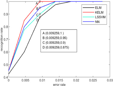
The recognition results of the four methods.

The recognition time includes the time for selecting samples randomly and the time for classification. Table 4 shows 20 groups data to compare the running times of different algorithms. The average time of LSSVM is 59.86, NN is 29.95; ELM is 11.12; and KELM is 4.16. Obviously, KELM is the fastest recognition method of the four ways.

Table 4

Recognition time (s) with the four methods

Group	NN	LSSVM	ELM	KELM
1	32.13	58.65	13.01	4.03
2	29.85	59.23	11.07	3.74
3	29.99	59.11	10.52	3.62
4	29.83	58.86	11.74	3.65
5	29.51	59.32	11.16	3.74
6	29.62	59.09	10.68	3.80
7	29.37	59.08	10.81	4.62
8	29.64	58.77	11.02	4.61
9	29.53	58.91	10.16	4.41
10	30.12	59.57	10.33	3.70
11	30.01	59.48	10.89	4.50
12	30.78	58.69	10.72	4.42
13	30.04	63.56	11.08	4.42
14	29.85	59.58	10.86	4.41
15	30.62	62.31	11.86	4.09
16	29.52	61.02	11.23	4.14
17	29.32	63.25	11.80	4.45
18	30.16	58.66	10.98	3.95
19	30.02	60.20	11.30	4.34
20	29.08	59.86	11.09	4.61
Average	29.95	59.86	11.12	4.16

From Table 2 and Table 3, it is easy to obtain that the average KELM accuracy can reach the highest. Though in some cases, the results of NN is better than KELM, there is little difference between the two methods. In addition, KELM needs less time for training and testing, and the time is in 5 seconds. Therefore, KELM is the most effective method in this test. In conclusion, by comparing the four classification algorithms from recognition accuracy and running speed, we can get that KELM is the most suitable method for NDT of wire rope.

6. Results and discussion

A detection device based on unsaturated magnetic excitation is exploited to capture the MFL signal. The proposed CSW and DD-DWT algorithm implement data noise reduction in MFL testing of wire rope; the proposed normalization rules can effectively realize the visualization of defects; KELM can classify the broken wires, which makes the learning extremely fast. Compared to the filtering algorithm and the algorithm in [11], the proposed algorithm in this paper provides good filtering performance. The classification method overcomes generalization and learning rate that exist in [11] and [17]. Compared to the results in [11], the recognition rate shown in Table 2 and Table 3 has high accuracy. In addition, with the utilization of the defect images as the input of the artificial neural networks for recognition, the identification process is simplified because the damage feature extraction is not required.

In this experiment, it is obvious that the algorithm combining KELM with CSW can effectively filter out the noise and realize accurate classification. However, during the data collection, different wire rope diameters result in different lift-off distance, which make the amplitude of the data with the same number of broken wires not exactly same. Thus, it is difficult to classify the broken wires. Due to the unknown sparsity in the reconstruction process of the sparse coefficient, the sparsity and the number of iterations are not adaptive, thus the number of sparsity and iteration need to be adjusted to ensure the minimum noise after restoration.

7. Conclusions

Under the device based on unsaturated magnetic excitation NDT, aiming at the problems in wire rope detection, an algorithm combining KELM with CSW was proposed in this paper. Based on ROMP and setting the constraint, the presented CSW filter inhibited the system noise and strand wave noise, which made the noise reduction more noticeable; To solve the problem that the defect image was not easy to be recognized, the normalization method proposed in this paper was used to process the image after segmentation and positioning, which improved the classification accuracy of broken wires. Compared with the traditional classification algorithms, KELM can quickly and accurately implement the classification of wire rope defects. This paper provides references for the service time and security of steel wire rope. However, the corrosion and wear of the wire rope will also affect the service life of the wire rope, which will become the focus of our future work.

References

Zhan

W.X.

, Research on singal process and quantiative recongnition method of broken wires wire rope, Ph.D. Qingdao Technological University, 2013.

Tan

X.J.

and Zhang

J.W.

, Evaluation of composite wire ropes using unsaturated magnetic excitation and reconstruction image with super-resolution, Applied Sciences 8(5) (2018), 767.

Tian

Zhou

Wang

and Meng

, Literature review of research on the technology of wire rope nondestructive inspection in china and abroad, EDP Sciences 22 (2015), 03025.

Kaur

Arora

Chhabra

and Sharma

, Characterization of LF and LMA signal of wire rope tester, International Journal of Advanced Research in Computer Science 8(5) (2017).

Tan

X.J.

and Zhang

J.W.

, Study of unsaturated magnetic image processing in wire rope aplication, International Symposium on. IEEE 2 (2017), 344–347.

Tian

Zhou

and Wang

, Literature review of research on the technology of wire rope nondestructive inspection in china and abroad, EDP Sciences 22 (2015), 03025, doi:10.1051/matecconf/20152203025.

Yan

Zhang

and Pan

, Online nondestructive testing for fine steel wire rope in electromagnetic interference environment, NDT & E International 92 (2017), 75–81, doi:10.1016/j.ndteint.2017.07.017.

Zhao

, Research on the technology of quantitative detection of local defect of wire rope by magnetic flux leakage, Ph.D. Harbin Institute of Technology, 2012.

Kaur

Gupta

and Aggarwal

, Non-destructive evaluation and development of a new wire rope tester using parallely magnetized NdFeB magnet segments, Journal of Nondestructive Evaluation 37(3) (2018), 61, doi:10.1007/s1092.

10.

Zhang

Tan

and Zheng

, Non-destructive detection of wire rope discontinuities from residual magnetic field images using the Hilbert-Huang transform and compressed sensing, Sensors 17(3) (2017), 608, doi:10.3390/s17030608.

11.

Zhang

and Tan

, Quantitative inspection of remanence of broken wire rope based on compressed sensing, Sensors 16(9) (2016), 1366, doi:10.3390/s16091366.

12.

Raisutis

Kazys

and Mazeika

, Propagation of ultrasonic guided waves in composite multi-wire ropes, Materials 9(6) (2016), 451, doi:10.3390/ma9060451.

13.

W.Z.

B.Z.

and Zheng

, Finite element analysis on the wire breaking rule of 1 × 7IWS steel wire rope, EDP Sciences 108 (2017), 01002, doi:10.1051/matecconf/201710801002.

14.

and Wang

, Damage location and numerical simulation for steel wire under torsion based on magnetic memory method, International Journal of Applied Electromagnetics and Mechanics (2019), 1–24, (Preprint).

15.

Feng

Kang

and Sun

, Influence of motion induced eddy current on the magnetization of steel pipe and MFL signal, International Journal of Applied Electromagnetics and Mechanics 52(1–2) (2016), 357–362.

16.

Cao

Y.N.

Zhang

D.L.

and Xu

D.G.

, Study on algorithms of wire rope localized flaw quantitative analysis based on three-dimensional magnetic flux leakage, Dianzi Xuebao (Acta Electronica Sinica) 35(6) (2007), 1170–1173.

17.

Zhang

Zheng

and Tan

, Recognition of broken wire rope based on remanence using EEMD and wavelet methods, Sensors 18(4) (2018), 1110, doi:10.3390/s18041110.

18.

Yan

Zhang

and Zhao

, Improve the signal to noise ratio and installation convenience of the inductive coil for wire rope nondestructive testing, NDT & E International 92 (2017), 221–227, doi:10.1016/j.ndteint.2017.09.005.

19.

Wang

H.Y.

Tian

and Meng

G.Y.

, Study on the adaptive wavelet threshold denoising method for coal mine hoisting wire rope signals based on novel thresholding function, Insight-Non-Destructive Testing and Condition Monitoring 60(2) (2018), 99–103, doi:10.1784/insi.2018.60.2.99.

20.

, Gap measurement of point machine using adaptive wavelet threshold and mathematical morphology, Sensors 16(12) (2016), 2006, doi:10.3390/s16122006.

21.

Cheng

Pan

Wang

, Research on MEMS gyroscope signal denoising based compressed sensing theory, Chinese Journal of Scientific Instrument 33(4) (2012), 769–773.

22.

Liu

Q.J.

, Time-frequency analysis and simulation of the watershed suspended sediment concentration based on the Hilbert-Huang transform (HHT) and artificial neural network (ANN) methods: A case study in the Loess Plateau of China, Catena 179 (2019), 107–118, doi:10.1016/j.catena.2019.03.042.

23.

Deng

and Huang

, ECG signal compressed sensing using the wavelet tree model, in: 2015 8th International Conference on Biomedical Engineering and Informatics (BMEI), IEEE, 2015, pp. 194–199, doi:10.1109/BMEI.2015.7401499.

24.

Zhang

Zhao

and Zhou

, Characterization of wire rope defects with gray level co-occurrence matrix of magnetic flux leakage images, Journal of Nondestructive Evaluation 32(1) (2013), 37–43, doi:10.1007/s10921-012-0156-6.

25.

Mallat

, A Wavelet Tour of Signal Processing, Elsevier, 1999.

26.

Mallat

, A theory for multiresolution signal decomposition: the wavelet representation, IEEE Transactions on Pattern Analysis & Machine Intelligence 7 (1989), 674–693, doi:10.1109/34.192463.

27.

J.J.

Han

and Mirko

, Microseismic and seismic denoising via ensemble empirical mode decomposition and adaptive thresholding, Geophysics 80(6) (2015), 69–S80, doi:10.1190/geo2014-0423.1.

28.

Gholipour

, Super resolution reconstruction in frequency, image, and wavelet domains to reduce through plane partial voluming in MRI, Medical Physics 42(12) (2015), 6919–6932, doi:10.1118/1.4935149.

29.

Qin

Y.N.

Gao

G.H.

and Lian

M.J.

, Wire rope fault diagnosis based on wavelet analysis and support vector machine (SVM), Trans Tech Publications 971 (2014), 1396–1399, doi:10.4028/www.scientific.net/AMR.971-973.1396.

30.

Meyer

and Wien

F.T.

, Support vector machines, The Interface to libsvm in package e1071, 28 (2015).

31.

Wan

and Li

, Diagnosis of elevator faults with LS-SVM based on optimization by K-CV, Journal of Electrical and Computer Engineering 70 (2015), doi:10.1155/2015/935038.

32.

Bui

D.T.

, Spatial prediction of rainfall-induced landslides for the Lao Cai area (Vietnam) using a hybrid intelligent approach of least squares support vector machines inference model and artificial bee colony optimization, Landslides 14(2) (2017), 447–458, doi:10.1007/s10346-016-0711-9.

33.

Cilimkovic

, Neural Networks and Back Propagation Algorithm, Vol. 15, Institute of Technology Blanchardstown, Blanchardstown Road North Dublin, 2015.

34.

Zhang

Zhao

and Zhou

, Quantitative inspection of wire rope discontinuities using magnetic flux leakage imaging, Materials Evaluation 70(7) (2012).

35.

Needell

and Roman

, Signal recovery from incomplete and inaccurate measurements via regularized orthogonal matching pursuit, arXiv preprint arXiv, 0712.1360 (2007).

36.

Roy

and Shailja

, A NLMS based approach for artifacts removal in multichannel EEG signals with ICA and double density wavelet transform, in: 2015 Fifth International Conference on Communication Systems and Network Technologies, IEEE, 2015. doi:10.1109/CSNT.2015.61.

37.

Huang

G.B.

Zhou

Ding

and Zhang

, Extreme learning machine for regression and multiclass classification, IEEE Trans. Systems, Man, Cybernetics: Part B 42(2) (2012), 513–529, doi:10.1109/TSMCB.2011.2168604.

38.

and Liu

, A kernel extreme learning machine algorithm based on improved particle swam optimization, Memetic Computing 9(2) (2017), 121–128, doi:10.1007/s12293-016-0182-5.

39.

Zhang

and Tian

, SVM and ELM: who wins? Object recognition with deep convolutional features from imagenet, in: Proceedings of ELM-2015 Volume 1, Springer, Cham, 2016, pp. 249–263. doi:10.1007/978-3-319-28397-5_20.

40.

Chen

and Su

, Spectral-spatial classification of hyperspectral image based on kernel extreme learning machine, Remote Sensing 6(6) (2014), 5795–5814, doi:10.3390/rs6065795.

41.

Zhang

, Multi-kernel extreme learning machine for EEG classification in brain-computer interfaces, Expert Systems with Applications 96 (2018), 302–310, doi:10.1016/j.eswa.2017.12.015.