Modeling and optimization of tubular linear permanent magnet eddy current brake with Halbach array

Abstract

This paper provides an analytical method for calculating the electromagnetic field of the tubular linear permanent magnet eddy current brake. The method of separating variables based on Fourier series is used to solve the boundary value problem, and the analytical solution of electromagnetic field is obtained. The braking force is obtained by calculating the Lorentz force. Then the accuracy of the analytical method is verified by comparing the analytical solutions with the solutions obtained by finite element method (FEM). In order to improve braking performance in a limited space, the parameter analysis is carried out to investigate the influence of various structural parameters on the braking characteristics. According to the results of parameter analysis, the range of design parameters is determined. Finally, a multi-objective optimization is applied to find the optimal design parameters of the eddy current brake. The braking force increases by 27% and the volume of permanent magnet decreases by 7.7% after optimization.

Keywords

Eddy current brake braking force finite element method genetic algorithm Halbach array

1. Introduction

Eddy current brakes are widely used in many industrial applications, such as aerospace applications, energy recovery system, high speed train braking systems, automobile suspension, and auxiliary braking devices, due to their advantages of simple structure, no mechanical contact, high reliability and easy maintenance [1–5]. Eddy current brakes can be divided into three types: electric excitation [6–8], permanent magnet [9–11], and hybrid excitation [12,13] eddy current brakes according to different excitation sources. The permanent magnet eddy current brake does not require additional power, is small in size and more reliable. Compared with planar linear eddy current brakes, tubular linear eddy current brakes have lower magnetic leakage, higher utilization of permanent magnets and no transverse edge effect [14].

The research methods of eddy current brake include analytical method and finite element method (FEM). The FEM can be applied to various complex structures, but it is time consuming. For some eddy current brakes with relatively regular structures, analytical methods can be used to analyze them. Bae et al. applied the Biot-Savart law and the Lorentz force formula to solve the magnetic flux density, then investigated the characteristics of eddy current damping when a permanent magnet was placed in a conductive tube. However, the predictability of this model is not accurate at high excitation frequency because the reaction of eddy current is not considered [15]. Ebrahimi et al. also studied the electromagnetic force of the tubular eddy current brake through Biot-Savart law and the Lorentz force formula, and considered the skin effect on the electromagnetic force. However, the eddy current reaction field was ignored and the effect of soft magnetic materials was not considered in the derivation [16]. In order to accurately account the eddy current reaction field, the electromagnetic field was calculated by solving Maxwell’s equations in some papers. Wang et al. deduced the magnetic field distribution of the tubular linear permanent magnet machines according to the magnetic vector potential and the cylindrical coordinate formula. Then he compared it with the finite element analysis to verify the results extensively [17]. However, only static results are given. Bianchi expressed the electromagnetic field problem by means of the magnetic scalar potential, then solved the Poisson’s equation and Laplace’s equation using separation variable method. In order to reduce the difficulty of solving the Poisson equation, they introduced a convenient approximation in the permanent magnet magnetization [18]. Magnetic scalar potentials can only be used in current-free regions, therefore cannot account the eddy current reaction field. Park et al. used the same approximation to express magnetization, then calculated the static air gap magnetic flux density of a tubular linear synchronous machine [19]. Amara et al. predicted the eddy current loss in the moving armature of a tubular permanent magnet machine using equivalent current sheets [20]. Although simplified models with equivalent current sheets may accurately predict the performance of some specific machines, Atallah et al. indicated that using equivalent current sheets can imply a loss of accuracy [21].

Most researches focus on the modeling process of eddy current brakes, then analyze the braking force characteristics and the influence of various structural parameters on the braking force characteristics [22–24]. According to different working conditions, there are different requirements for the performance of ECB. In order to play a better role in specific application scenarios, it is necessary to coordinate and match ECB comprehensively. However, the structural parameters of the ECB have not been further optimized to achieve the desired braking force characteristics in those researches. In addition, there are more than one indicator for evaluating the braking force characteristics. Multi-objective optimization techniques can be used to deal with multi-objective optimization problems.

In this paper, the reaction of the eddy current field is fully considered, and the analytical model of a tubular linear permanent magnet eddy current brake is established based on the magnetic vector potential and the cylindrical coordinate system. The residual magnetism model is used to represent the permanent magnet instead of the equivalent current sheets model because of the equivalent current sheets model is not accurate for all mechanical topologies. Then the boundary value problem of partial differential equations is solved by the method of separating variables and Fourier series. Analytical expressions of electromagnetic fields under quasi-static conditions are obtained. The accuracy of the analytical model is verified by comparison with the results calculated by the FEM. Through harmonic analysis, it is found that the braking force with sufficient accuracy can be obtained by calculating the 1, 5 and 9 orders. When the harmonic order increases, it is necessary to increase the number of digits of numerical calculation to obtain accurate results. Considering that the optimization process requires a lot of iterative calculations and the performance of ECB is difficult to evaluate with a single index, multi-objective optimization of the ECB is carried out by establishing a surrogate model and combining with GA.

2. Analytical model

2.1. Analytical modeling

Fig. 1.

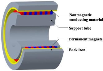
Structure of the tubular linear permanent magnet eddy current brake with Halbach array.

Figure 1 shows a schematic of a tubular linear permanent magnet eddy current brake with Halbach array. The Halbach array can increase the magnetic flux density on one side and decrease it on the other. Therefore, the magnetic permeability of the support tube with Halbach array has a small impact on the braking force. The permanent magnets are installed on the support tube. The conductive tube is covered by back iron, which can significantly enhance the air gap magnetic flux density. When the support tube moves, eddy current is generated in the conductive tube. Then the eddy current interacts with the magnetic field to generate a braking force.

Fig. 2.

Simplified analytical model.

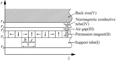
Figure 2 shows the simplified analytical model. The analysis will be performed in a cylindrical coordinate system (r, φ, z) fixed to the permanent magnet. r ₀ and r ₁ are the inner and outer radii of the support tube; r ₂ is the outer radii of the permanent magnets; r ₃ and r ₄ are the inner and outer radii of the nonmagnetic conductive tube. b and c are the axial length of axial magnetization and radial magnetization of the permanent magnets. τ is the pole pitch. h _m, δ and d are the radial thickness of permanent magnets, air gap and nonmagnetic conductive tube, respectively. In the particular machine under consideration, the permanent magnets are mounted on a high strength steel tube. In order to obtain an analytical solution for the electromagnetic field, the following assumptions are made:

The z axial end effect is ignored so that the electromagnetic field is periodic distributed along the z axis.

The relative permeability of ferromagnetic materials is constant and the radial thickness of back iron is infinite. For it has been observed that this approximation does not modify the performance prediction of the eddy current brake when the radial thickness of the back iron is large [25].

The current density distribution is supposed directed only along the z axis. Therefore, the electromagnetic field distribution can be described as a two-dimensional problem.

The analytical model is divided into five sub-regions. Assume that only region IV has a non-zero conductivity. The assumption that the conductivity of region V is zero will be explained in Section 2.2. So in regions I, II, III and V, J = 𝛻 × H = 0. J and H denote the current density and magnetic field strength. The governing equation expressed in terms of the magnetic vector potential A (using a Coulomb gauge 𝛻 ⋅ A = 0) is $$\begin{eqnarray}\displaystyle {\nabla}^{2}\mathbf{A}^{\text{I},\text{III},\text{V}}=0. & & \displaystyle\end{eqnarray}$$(1)

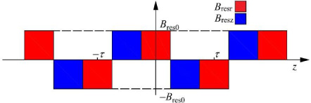
The constitutive relation of permanent magnet can be described by residual magnetism $\begin{eqnarray}\displaystyle \text{} & \text{} & \displaystyle \mathbf{B}={\mu}_{0}\mathbf{H}+\mathbf{B}_{res}\end{eqnarray}$ (2) $\begin{eqnarray}\displaystyle \text{} & \text{} & \displaystyle \mathbf{B}_{res}=\mathbf{B}_{resr}+\mathbf{B}_{resz}\end{eqnarray}$ (3) where B, B _res, B _resr and B _resz are the magnetic flux density, remanence, radial remanence and axial remanence, respectively. μ₀ is the permeability of vacuum. The waveform of the residual magnetism is shown in Fig. 3. As shown in Fig. 3, the two residual flux density components aren’t simultaneously nonzero. B _res0 is the value of the residual magnetism.

Fig. 3.

Waveform of residual magnetism.

The rectangular waveform can be expressed by Fourier series $\begin{eqnarray}\displaystyle \left\{\begin{array}{@{}l@{}}\displaystyle \mathbf{B}_{resr}(z)=\mathop{\sum }_{n}\mathbf{B}_{resr}^{n}\cdot e^{jmz}\\ \displaystyle \mathbf{B}_{resz}(z)=\mathop{\sum }_{n}\mathbf{B}_{resz}^{n}\cdot e^{jmz}\end{array}\right. & & \displaystyle\end{eqnarray}$ (4) where m = nπ∕τ.

Therefore, the governing equations of region II is $\begin{eqnarray}\displaystyle {\nabla}^{2}\mathbf{A}^{\text{II}}=-({\nabla}\times \mathbf{B}_{res}). & & \displaystyle\end{eqnarray}$ (5) The conductivity of the nonmagnetic conductive tube is σ. The current density is $\begin{eqnarray}\displaystyle \mathbf{J}={\sigma}\mathbf{E} & & \displaystyle\end{eqnarray}$ (6) where E is the electric field strength. According to Faraday’s law $\begin{eqnarray}\displaystyle {\nabla}\times \mathbf{E}=-{\displaystyle \frac{\partial \mathbf{B}}{\partial t}}. & & \displaystyle\end{eqnarray}$ (7) So the governing equation can be derived as $\begin{eqnarray}\displaystyle {\nabla}^{2}\mathbf{A}^{\text{IV}}={\mu}_{0}{\sigma}v{\displaystyle \frac{\partial \mathbf{A}}{\partial z}} & & \displaystyle\end{eqnarray}$ (8) where v is the relative speed of stator and mover.

Since all the electromagnetic quantities are periodic with the pole pitch τ, the magnetic vector potential can be written as [25] $\begin{eqnarray}\displaystyle \mathbf{A}(r,z)=\mathop{\sum }_{n}\mathbf{A}_{n}(r)\cdot e^{jmz}. & & \displaystyle\end{eqnarray}$ (9) Substituting (9) for the (1), (5) and (8) and substituting (4) for the (5) gives the following equations $\begin{eqnarray}\displaystyle \text{} & \text{} & \displaystyle {\displaystyle \frac{\partial ^{2}A_{n}^{\text{I},\text{III},\text{V}}(r)}{\partial r^{2}}}+{\displaystyle \frac{\partial A_{n}^{\text{I},\text{III},\text{V}}(r)}{r\partial r}}-m^{2}A_{n}^{\text{I},\text{III},\text{V}}(r)-{\displaystyle \frac{A_{n}^{\text{I},\text{III},\text{V}}(r)}{r^{2}}}=0\end{eqnarray}$ (10) $\begin{eqnarray}\displaystyle \text{} & \text{} & \displaystyle {\displaystyle \frac{\partial ^{2}A_{n}^{\text{II}}(r)}{\partial r^{2}}}+{\displaystyle \frac{\partial A_{n}^{\text{II}}(r)}{r\partial r}}-m^{2}A_{n}^{\text{II}}(r)-\frac{A_{n}^{\text{II}}(r)}{r^{2}}=-jmB_{resr}^{n}\end{eqnarray}$ (11) $\begin{eqnarray}\displaystyle \text{} & \text{} & \displaystyle {\displaystyle \frac{\partial ^{2}A_{n}^{\text{IV}}(r)}{\partial r^{2}}}+{\displaystyle \frac{\partial A_{n}^{\text{IV}}(r)}{r\partial r}}-m^{2}A_{n}^{\text{IV}}(r)-{\displaystyle \frac{A_{n}^{\text{IV}}(r)}{r^{2}}}=jm{\mu}_{0}{\sigma}vA_{n}^{\text{IV}}(r).\end{eqnarray}$ (12)

Solve the above ordinary differential equation. Then the magnetic vector potential of each region described by the modified Bessel equations are obtained. $\begin{eqnarray}\displaystyle \text{} & \text{} & \displaystyle A_{n}^{\text{I},\text{III},\text{V}}(r,z)=[\text{C}_{n}^{\text{I},\text{III},\text{V}}\text{I}_{1}(mr)+\text{D}_{n}^{\text{I},\text{III},\text{V}}\text{K}_{1}(mr)]e^{jmz}\end{eqnarray}$ (13) $\begin{eqnarray}\displaystyle \text{} & \text{} & \displaystyle A_{n}^{\text{II}}(r,z)=\left[\text{C}_{n}^{\text{II}}\text{I}_{1}(mr)+\text{D}_{n}^{\text{II}}\text{K}_{1}(mr)-\frac{j{\pi}B_{resr}^{n}\text{L}_{1}(mr)}{2m}\right]e^{jmz}\end{eqnarray}$ (14) $\begin{eqnarray}\displaystyle \text{} & \text{} & \displaystyle A_{n}^{\text{IV}}(r,z)=[\text{C}_{n}^{\text{IV}}\text{I}_{1}(m^{\prime }r)+\text{D}_{n}^{\text{IV}}\text{K}_{1}(m^{\prime }r)]e^{jmz}\end{eqnarray}$ (15) where $m^{\prime }=\sqrt{jm{\mu}_{0}{\sigma}v+m^{2}}$ , I ₁, K ₁ and L ₁ are the first-order modified Bessel functions of the first and the second kind and the first-order modified Struve function, respectively. $\text{C}_n^{\text{I}-\text{V}}$ and $\text{D}_{n}^{\text{I}-\text{V}}$ are complex constants depending on following boundary conditions. $\begin{eqnarray}\displaystyle \text{} & \text{} & \displaystyle A^{\text{I}}(r,z)=0|r=r_{0}\end{eqnarray}$ (16) $\begin{eqnarray}\displaystyle \text{} & \text{} & \displaystyle A^{\text{V}}(r,z)=0|r\rightarrow \infty\end{eqnarray}$ (17) $\begin{eqnarray}\displaystyle \text{} & \text{} & \displaystyle A_{n}^{\text{I}}(r)=A_{n}^{\text{II}}(r)|r=r_{1}\end{eqnarray}$ (18) $\begin{eqnarray}\displaystyle \text{} & \text{} & \displaystyle A_{n}^{\text{II}}(r)=A_{n}^{\text{III}}(r)|r=r_{2}\end{eqnarray}$ (19) $\begin{eqnarray}\displaystyle \text{} & \text{} & \displaystyle A_{n}^{\text{III}}(r)=A_{n}^{\text{IV}}(r)|r=r_{3}\end{eqnarray}$ (20) $\begin{eqnarray}\displaystyle \text{} & \text{} & \displaystyle A_{n}^{\text{IV}}(r)=A_{n}^{\text{V}}(r)|r=r_{4}\end{eqnarray}$ (21) $\begin{eqnarray}\displaystyle \text{} & \text{} & \displaystyle {\displaystyle \frac{1}{{\mu}_{1}}}\left[A_{n}^{\text{I}}(r)+{\displaystyle \frac{\partial }{\partial r}}(rA_{n}^{\text{I}}(r))\right]=A_{n}^{\text{II}}(r)+\frac{\partial }{\partial r}(rA_{n}^{\text{II}}(r))-rB_{resz}|r=r_{1}\end{eqnarray}$ (22) $\begin{eqnarray}\displaystyle \text{} & \text{} & \displaystyle {\displaystyle \frac{\partial }{\partial r}}(rA_{n}^{\text{II}}(r))-rB_{resz}={\displaystyle \frac{\partial }{\partial r}}(rA_{n}^{\text{III}}(r))|r=r_{2}\end{eqnarray}$ (23) $\begin{eqnarray}\displaystyle \text{} & \text{} & \displaystyle {\displaystyle \frac{\partial }{\partial r}}(rA_{n}^{\text{III}}(r))={\displaystyle \frac{\partial }{\partial r}}(rA_{n}^{\text{IV}}(r))|r=r_{3}\end{eqnarray}$ (24) $\begin{eqnarray}\displaystyle \text{} & \text{} & \displaystyle A_{n}^{\text{IV}}(r)+{\displaystyle \frac{\partial }{\partial r}}(rA_{n}^{\text{IV}}(r))={\displaystyle \frac{1}{{\mu}_{5}}}\left[A_{n}^{\text{V}}(r)+{\displaystyle \frac{\partial }{\partial r}}(rA_{n}^{\text{V}}(r))\right]|r=r_{4}\end{eqnarray}$ (25) where μ₁ and μ₅ are the relative permeability of the support tube and the back iron. Assuming the values of μ₁ and μ₅ are equal to 600.

The boundary conditions ((16)) and ((17)) indicate that the radial component of magnetic flux density vanishes at r ₀ and infinity. Then the equations ((18))–((21)) ensure the continuity of the normal component of magnetic flux density at the interface of different regions. Equation ((22))–((25)) ensure the continuity of the tangential component of the magnetic field strength. Substituting ((13))–((15)) into the boundary conditions results in a system that can be written as ((26)). $$\begin{eqnarray}\displaystyle \text{} & \text{} & \displaystyle \hspace{-18.0pt}\left[\begin{array}{@{}ccccccccc@{}}\text{I}_{1}(mr_{0}) & \text{K}_{1}(mr_{0}) & 0 & 0 & 0 & 0 & 0 & 0 & 0\\ \text{I}_{1}(mr_{\mathbf{1}}) & \text{K}_{1}(mr_{1}) & -\text{I}_{1}(mr_{1}) & -\text{K}_{1}(mr_{1}) & 0 & 0 & 0 & 0 & 0\\ \text{I}_{0}(mr_{1})/{\mu}_{5} & -\text{K}_{0}(mr_{1})/{\mu}_{5} & -\text{I}_{0}(mr_{1}) & \text{K}_{0}(mr_{1}) & 0 & 0 & 0 & 0 & 0\\ 0 & 0 & \text{I}_{1}(mr_{2}) & \text{K}_{1}(mr_{2}) & -\text{I}_{1}(mr_{2}) & -\text{K}_{1}(mr_{2}) & 0 & 0 & 0\\ 0 & 0 & \text{I}_{0}(mr_{2}) & -\text{K}_{0}(mr_{2}) & -\text{I}_{0}(mr_{2}) & \text{K}_{0}(mr_{2}) & 0 & 0 & 0\\ 0 & 0 & 0 & 0 & \text{I}_{1}(mr_{3}) & \text{K}_{1}(mr_{3}) & -\text{I}_{1}(mr_{3}^{\prime }) & -\text{K}_{1}(mr_{3}^{\prime }) & 0\\ 0 & 0 & 0 & 0 & \text{I}_{0}(mr_{3}) & -\text{K}_{0}(mr_{3}) & -\text{I}_{0}(mr_{3}^{\prime }) & \text{K}_{0}(mr_{3}^{\prime }) & 0\\ 0 & 0 & 0 & 0 & 0 & 0 & \text{I}_{1}(mr_{4}^{\prime }) & \text{K}_{1}(mr_{4}^{\prime }) & -\text{I}_{1}(mr_{4})\\ 0 & 0 & 0 & 0 & 0 & 0 & \text{I}_{0}(mr_{4}^{\prime }) & -\text{K}_{0}(mr_{4}^{\prime }) & \text{K}_{1}(mr_{4})/{\mu}_{5}\end{array}\right]\nonumber\\ \displaystyle \text{} & \text{} & \displaystyle \quad \left[\begin{array}{@{}c@{}}\text{C}_{n}^{\text{I}}\\[5.0pt] \text{D}_{n}^{\text{I}}\\[5.0pt] \text{C}_{n}^{\text{II}}\\[5.0pt] \text{D}_{n}^{\text{II}}\\[5.0pt] \text{C}_{n}^{\text{III}}\\[5.0pt] \text{D}_{n}^{\text{III}}\\[5.0pt] \text{C}_{n}^{\text{IV}}\\[5.0pt] \text{D}_{n}^{\text{IV}}\\[5.0pt] \text{D}_{n}^{\text{V}}\end{array}\right]=\left[\begin{array}{@{}c@{}}0\\ -j{\pi}B_{resr}^{n}\text{L}_{1}(mr_{1})/2m\\[5.0pt] -(j{\pi}B_{resr}^{n}\text{L}_{0}(mr_{1})+2B_{resz}^{n})/2m\\[5.0pt] j{\pi}B_{resr}^{n}\text{L}_{1}(mr_{2})/2m\\[5.0pt] (j{\pi}B_{resr}^{n}\text{L}_{0}(mr_{2})+2B_{resz}^{n})/2m\\[5.0pt] 0\\ 0\\ 0\\ 0\end{array}\right].\end{eqnarray}$$(26) The solutions of unknown constants are lengthy expressions of modified Bessel functions and modified Struve functions. The $\text{C}_{n}^{\text{IV}}$ and $\text{D}_{n}^{\text{IV}}$ are given in Appendix.

According to the solution of the magnetic vector potential, the magnetic flux density and eddy current distribution in the nonmagnetic conductive tube can be obtained $$\begin{eqnarray}\displaystyle \text{} & \text{} & \displaystyle \mathbf{J}^{\text{IV}}=-{\sigma}v{\displaystyle \frac{\partial \mathbf{A}^{\text{IV}}}{\partial z}}\end{eqnarray}$$(27) $$\begin{eqnarray}\displaystyle \text{} & \text{} & \displaystyle j_{n}^{\text{IV}}(r,z)=jm{\sigma}v[\text{C}_{n}^{\text{IV}}\text{I}_{1}(m^{\prime }r)+\text{D}_{n}^{\text{IV}}\text{K}_{1}(m^{\prime }r)]e^{jmz}\end{eqnarray}$$(28) $$\begin{eqnarray}\displaystyle \text{} & \text{} & \displaystyle \mathbf{B}={\nabla}\times \mathbf{A}\end{eqnarray}$$(29) $$\begin{eqnarray}\displaystyle \text{} & \text{} & \displaystyle B_{rn}^{\text{IV}}(r,z)=-jm[\text{C}_{n}^{\text{IV}}\text{I}_{1}(m^{\prime }r)+\text{D}_{n}^{\text{IV}}\text{K}_{1}(m^{\prime }r)]e^{jmz}\end{eqnarray}$$(30) $$\begin{eqnarray}\displaystyle \text{} & \text{} & \displaystyle B_{zn}^{\text{IV}}(r,z)=m[\text{C}_{n}^{\text{IV}}\text{I}_{0}(m^{\prime }r)+\text{D}_{n}^{\text{IV}}\text{K}_{0}(m^{\prime }r)]e^{jmz}.\end{eqnarray}$$(31)

Finally, the Lorentz force can be obtained $\begin{eqnarray}\displaystyle \mathbf{F}_{z}=2{\pi}\displaystyle \int _{-{\tau}}^{{\tau}}\displaystyle \int _{r_{3}}^{r_{4}}\mathbf{B}^{\text{IV}}\times \mathbf{J}^{\text{IV}}\mathit{rd}zdr. & & \displaystyle\end{eqnarray}$ (32) The integral (32) contains a lengthy combination of Bessel functions, which is difficult or even impossible to solve analytically and hence is solved numerically. Following model verification, the Lorentz force of one period of the conductive tube is calculated for comparison, as shown in Fig. 4.

2.2. Model validation

The analytical model is verified by comparing the analytical results with numerical solution obtained by the FEM. The calculations are performed using the parameters given in Table 1. The axial length of an actual permanent magnet array is finite. In order to eliminate end effects, the braking force calculated by the finite element model comes from one period of the permanent magnet array. The FEM analysis is implemented using the COMSOL Multiphysics software. Choose the AC/DC module to solve the Maxwell equations formulated using vector magnetic potential to establish a two-dimensional axisymmetric finite element model. The local finite element model is shown in Fig. 4. The setting of constitutive relations is consistent with the analytical model. Give the conductor tube and the back iron a very small acceleration to calculate the braking force under quasi-static. Figure 5 shows the magnetic field distribution at 0 m/s and 20 m/s. It can be seen that in the static state, the magnetic induction lines pass through the conductor cylinder almost perpendicularly from the permanent magnet magnetized radially. When the eddy current brake is working, due to the reaction of the eddy current field, the magnetic field distribution is distorted.

Fig. 4.

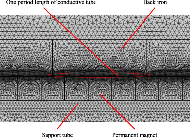
Local finite element model.

Table 1

Parameters of the eddy current brake used in the calculations

Parameter	Description	Value
d	Conductor plate thickness	1 mm
δ	Air gap length	0.5 mm
h _m	Length of permanent magnet	20 mm
r ₁	Inner radius of permanent magnet	167 mm
r ₀	Inner radius of support tube	77.5 mm
b	Axial length of axially magnetized permanent magnet	20 mm
c	Axial length of radially magnetized permanent magnet	20 mm
σ	Conductivity of conductor	24.6 MS/m
B _res0	Remanence of permanent magnet	1.1 T
μ₁	Relative permeability of support tube	600
μ₅	Relative permeability of back iron	600

Fig. 5.

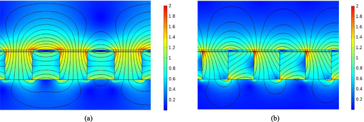
Magnetic flux density distribution at the speed of 0 m/s (a) and 20 m/s (b).

Figure 6 compares the analytical results and the finite element results of B _r in the middle of the nonmagnetic conductive tube (r = r ₃ + d∕2), whereas Fig. 7 compares the B _z. The analytical results and the finite element results very good agreement. It can be observed that, consistent with the results shown in Fig. 5, the magnetic flux density of the static magnetic field forms a platform at the permanent magnet magnetized radially. The reaction of the eddy current field will cause the platform to disappear into an extreme point, showing the effect of field suppression.

Fig. 6.

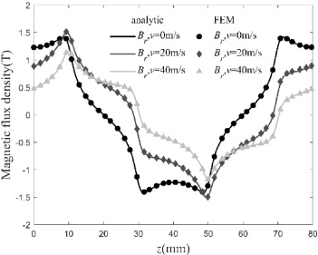
Comparison of magnetic flux density B _r as functions of z at r = r ₃ + d∕2.

Fig. 7.

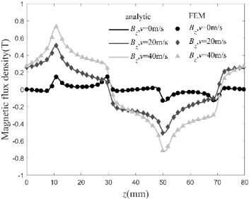
Comparison of magnetic flux density B _z as functions of z at r = r ₃ + d∕2.

The curves of current density as functions of v at different points in the middle of nonmagnetic conductive tube are shown in Fig. 8. The analytical and finite element curves also show excellent consistency. Due to the distortion of magnetic induction intensity distribution, the eddy current distribution has also changed, and the peak position of the eddy current has shifted.

Fig. 8.

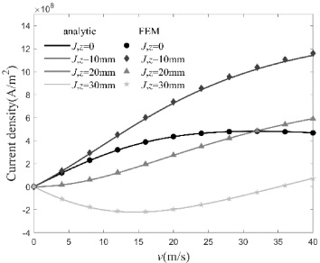
Comparison of current density as functions of v at different points (r = r ₃ + d∕2).

Fig. 9.

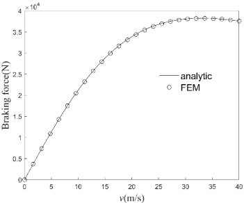
Comparison of braking force as functions of v.

Figure 9 is braking force as the function of speed. Since the analytical expression of the magnetic field distribution contains a lengthy combination of Bessel functions, the braking force is obtained by numerical integration. As the harmonic order increases, in order to obtain accurate numerical solutions of the boundary condition equations, the number of digits in the numerical calculation process must be increased. Otherwise, the result may be wrong. This is discussed in detail in the next section. At low speeds, the eddy current damping coefficient is roughly linear. Due to the reaction of eddy current, the magnetic field distribution is distorted, the damping coefficient changes from linear to non-linear, and the braking force has a peak value. This analytical method can accurately describe this physical phenomenon. Comparing the calculation results of the analytical method with the results of the FEM shows that the two methods are in good agreement. Therefore, the accuracy of the analytical method is verified. The quantitative comparison of the error between the braking force obtained by the analytical method and the braking force obtained by the FEM in Fig. 8 is discussed in Section 2.3.

When the conductivity of region V is 11.2 MS/m, the braking force as the function of speed is shown in Fig. 10. It can be seen that eddy currents mainly appear in region IV, so the assumption that the conductivity of region V is zero is reasonable.

Fig. 10.

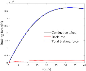
Comparison of braking force of different tubes.

2.3. Limitations of analytical model

The analytical model based on Fourier series exhibits a similar problem. The accuracy of the analytical model is related to the amount of harmonic orders used. Since the computational time of the model mainly depends on the amount of harmonic orders, considering the computation cost, the amount of harmonic orders to be calculated cannot be infinite. When the analytical model is actually used, the amount of harmonic orders calculated should be determined according to the numerical accuracy and computational time. Moreover, the amount of harmonic orders required to calculate the magnetic flux density, eddy current density, and braking force may be different.

A method to reduce computational time is to perform a preliminary harmonic analysis of the machine under study to exclude a series of harmonic orders. This reduces the amount of harmonic orders that need to be calculated, thus reducing computational time. As shown in Fig. 3, the spatial distribution of the remanence is symmetrical about r axis. $B_{resr}^{n}$ and $B_{resz}^{n}$ can be expressed as $\begin{eqnarray}\displaystyle \text{} & \text{} & \displaystyle B_{resr}^{n}={\displaystyle \frac{B_{res0}}{n{\pi}}}\left(\sin \left({\displaystyle \frac{n{\pi}}{4}}\right)+\sin \left({\displaystyle \frac{3n{\pi}}{4}}\right)\right)\end{eqnarray}$ (33) $\begin{eqnarray}\displaystyle \text{} & \text{} & \displaystyle B_{resz}^{n}={\displaystyle \frac{jB_{res0}}{n{\pi}}}\left(\cos \left({\displaystyle \frac{n{\pi}}{4}}\right)-\cos \left({\displaystyle \frac{3n{\pi}}{4}}\right)\right).\end{eqnarray}$ (34)

Obviously, the harmonic orders can exclude even terms according to (33) and (34). As can been observed from Fig. 11, the main harmonic orders in the radial magnetic flux density are first, fifth and ninth orders. The harmonic amplitudes of the third, seventh, eleventh etc. are very small and can be ignored.

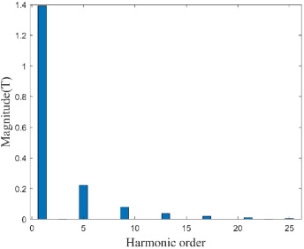
The relative difference between analytical (ANA) and FEM results are quantified using the normalized root mean square deviation (NRMSD) [26]. $\begin{eqnarray}\displaystyle \text{NRMSD}={\displaystyle \frac{\sqrt{\displaystyle \frac{1}{2{\tau}}\int _{-{\tau}}^{{\tau}}(y_{FEM}-y_{ANA})^{2}}}{\max (y_{FEM})-\min (y_{FEM})}}100\% & & \displaystyle\end{eqnarray}$ (35) where y _FEM is the value calculated by FEM and y _ANA is obtained from ANA.

Fig. 11.

Harmonic distribution of radial magnetic flux density in a conductive tube.

Fig. 12.

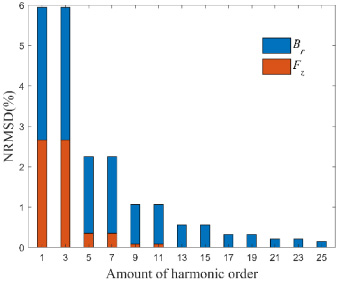
NRMSD of B _r and F _z at different amount of harmonic order.

Figure 12 shows the NRMSD of braking force is only 0.083% with the highest order reaching nine, whereas the NRMSD of radial magnetic flux density is 0.15% with the highest order reaching twenty-five. It can also been seen that the contribution of third, seventh, eleventh etc. harmonics to the result can be neglected.

For an increased harmonic number, solving the equations for the boundary conditions results in ill-conditioned system of equations; hence, the solution becomes inaccurate [27]. In addition, there are inevitably rounding errors in the numerical calculation process. The expressions of the unknown coefficient $\text{C}_{n}^{\text{I}-\text{V}}$ and $\text{D}_{n}^{\text{I}-\text{V}}$ calculated by system (26) includes various combinations of Bessel functions and Struve functions. For example, the $\text{C}_{n}^{\text{IV}}$ has a combination of special functions as shown below $\begin{eqnarray}\displaystyle \text{L}_{1}(mr_{2})\text{I}_{0}(mr_{2})-\text{L}_{0}(mr_{2})\text{I}_{1}(mr_{2}). & & \displaystyle\end{eqnarray}$ (36)

For (36), sufficient number of digits are needed to obtain correct results. The larger the harmonic order, the more digits are required, otherwise the result of (36) is zero. For the solution of system (26), an increase in speed can also lead to inaccurate solutions. As the harmonic order and speed increase, in order to obtain an accurate solution, the number of digits in the numerical calculation process must be increased. However the increase in the number of digits will undoubtedly increase the time consumed for computation.

2.4. Experiment

In order to verify the accuracy of analytical method and FEM, a small prototype is manufactured. The dominating specifications of the prototype are summarized in Table 2. The experimental device is depicted in Fig. 13. The air-hammer hits the slider to give speed to the moving part of the ECB. Figure 14 shows the test results of the small prototype. It can be seen that the test results are in good agreement with the FEM results. The accuracy of the FEM is validated. The analytical method does not consider the end effect, so the calculated result is larger than that of the FEM.

Fig. 13.

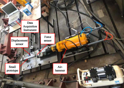
Experimental device of the testing system.

Table 2

Specifications of small prototype

Parameter	Description	Value
d _s	Conductor plate thickness	2 mm
δ_s	Air gap length	0.5 mm
h _ms	Length of permanent magnet	13.5 mm
r _1s	Inner radius of permanent magnet	12 mm
b _s	Axial length of axially magnetized permanent magnet	13.5 mm
c _s	Axial length of radially magnetized permanent magnet	13.5 mm
σ_s	Conductivity of conductor	28 MS/m
B _res0s	Remanence of permanent magnet	0.9 T
n	Number of permanent magnets	9

Fig. 14.

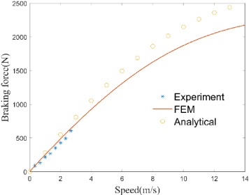
Comparison between FEM, analytical, and experimental results.

3. Parametric analysis and optimization

The reasonable design of the eddy current brake can save materials and improve performance. Optimizing structural parameters requires a lot of calculations. Considering the computing cost, an approximate model is established instead of the original model.

3.1. Parametric analysis

The performance indicators for evaluating eddy current brakes include damping coefficient at low speed, peak braking force, critical speed (speed corresponding to peak braking force), damping density, and braking force density, where damping density is defined as the ratio of the damping coefficient at low speed over the permanent magnets volume and braking force density is defined as the ratio of the peak braking force over the permanent magnets volume. $\begin{eqnarray}\displaystyle \text{} & \text{} & \displaystyle DD={\displaystyle \frac{c_{d}}{V_{m}}}\end{eqnarray}$ (37) $\begin{eqnarray}\displaystyle \text{} & \text{} & \displaystyle FD={\displaystyle \frac{F_{z}}{V_{m}}}\end{eqnarray}$ (38) where DD represents the damping density, c _d is the damping coefficient at low speed and is a constant, V _m is the permanent magnets mass and FD denotes the braking force density.

The performance of the eddy current brake is related to many structural parameters, such as the axial length of axially magnetized and radially magnetized permanent magnets and the radial thickness of permanent magnets and nonmagnetic conductive tube. It is necessary to analyze the relationship between structural parameters and braking characteristics, before optimizing structural parameters. Then the design parameters and corresponding value ranges are determined according to the results of the parameter analysis.

As shown in Fig. 15, the increase of d leads to the increase of damping coefficient c. Nevertheless, the damping coefficient will not increase indefinitely, for an increase in d means an increase in magnetic resistance, and the existence of skin effect. On the other hand, the critical speed and the peak braking force are reduced with the increased eddy current reaction.

In Fig. 16, the braking force curves are shown for different permanent magnets thickness h _m. It can be seen that the increase in h _m results in an increase in the peak braking force and an increase in the damping coefficient. However, there are optimum values of h _m for the braking force density and the damping density, because the magnitude of the increase in braking force density and damping density will gradually decrease.

Fig. 15.

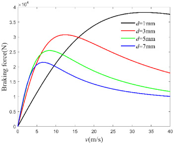
Braking force as functions of v at different conductor plate thicknesses.

Fig. 16.

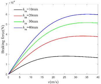
Braking force as functions of v at different permanent magnets thicknesses.

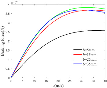
As can be seen from Fig. 17, b clearly has the optimal value. The increase in b increases both the magnetomotive force and the reluctance. Properly increasing b can effectively, but not infinitely increase the air gap magnetic flux density.

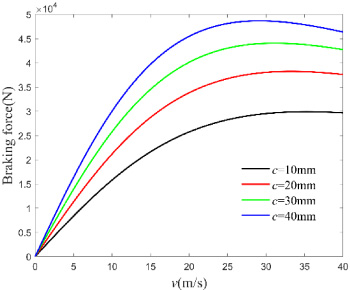
It can been observed in Fig. 18 that the relationship between c and braking force characteristics is similar to that between h _m and braking force characteristics. Both are mainly changes in the braking force characteristics caused by changing the volume of the radially magnetized permanent magnet and the size of the eddy current region. Therefore, there is also an optimal value of c for the braking force density and damping density.

Fig. 17.

Braking force as functions of v at different axial lengths of axial magnetized permanent magnets.

Fig. 18.

Braking force as functions of v at different axial lengths of radial magnetized permanent magnets.

3.2. Optimization

In the previous section, the influence of design parameters on braking force characteristics was analyzed. Different work scenarios require suitable braking force characteristics. In the particular eddy current brake considered, assuming the maximum working speed does not exceed 13 m/s. So 13 m/s is selected as the working speed, which is the end of the profile of the moving speed, related to braking force, during actual work. The entire profile of braking force needs to be considered when optimizing the design. Therefore, this paper chooses the damping coefficient at low speed and the braking force at working speed to characterize the overall profile. The damping coefficient represents the speed at which the braking force rises, and the braking force corresponding to the working speed represents the braking force at the end of the profile. The working speed of the original structure is lower than the critical speed, that is, the braking force at the working speed of the original structure is the maximum braking force during actual work. Therefore, the entire profile of the moving speed, related to braking force, can be estimated based on the damping coefficient and the braking force under the working speed. The braking force at working speed and the damping coefficient can be increased by reducing some evaluation indicators, such as the critical speed and the peak braking force.

The sensitivities of the braking force at the working speed and the damping coefficient with respect to b and c are shown in Figs 19 and 20. It can be seen that compared to b, the braking force and damping coefficient are more sensitive to c. In the specific combination of b and c, the braking force is inversely related to b, which must be avoided.

Fig. 19.

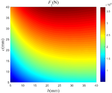
Sensitivity of F _z with respect to b and c.

Fig. 20.

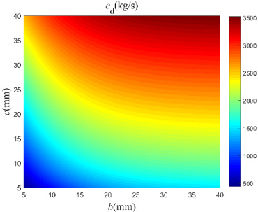
Sensitivity of c _d with respect to b and c.

In this study, the optimization is performed using back-propagation (BP) neural network surrogate model, because the FEM is time consuming, the unknown coefficients in the analytical expressions are too verbose and complex, and (32) it is difficult to give an analytical expression. The genetic algorithm optimization solving strategy based on the back-propagation neural network surrogate model is shown in Fig. 21.

Fig. 21.

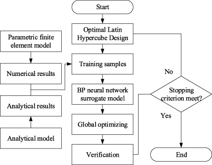
Genetic algorithm optimization solving strategy based on the back-propagation neural network surrogate model.

Table 3 shows the design variables and corresponding ranges. The inner diameter of the permanent magnet and the thickness of the back iron remain unchanged according to the actual work needs. The optimization goal is to increase the braking force at the working speed and damping coefficient, while reducing the volume of the permanent magnet. In order to ensure that the back iron is not magnetically saturated, the air gap magnetic flux density B _g is limited to less than 1.46 T. So the multi-objective optimization problem can be described as $\begin{eqnarray}\displaystyle \left\{\begin{array}{@{}l@{}}\max F_{z}(x),\min V_{m}(x),\max c_{d}(x)\\[5.0pt] x=\left[\begin{array}{@{}cccc@{}}b & c & d & h_{m}\end{array}\right]^{\text{T}}\\[5.0pt] \text{subject to}\\ B_{g}(x)\leq 1.46∼\text{T},F_{z}(x)\geq F_{z}(x_{i}),V_{m}(x)\leq V_{m}(x_{i})\\[5.0pt] x\in D\end{array}\right. & & \displaystyle\end{eqnarray}$ (39) where x _i is the initial design variables and D is the design space.

Table 3

Design variables

Parameter	Initial	Range
b (mm)	20	10–35
c (mm)	20	10–40
d (mm)	1	1–3
h _m (mm)	20	15–40

Sample points are obtained using the optimal Latin square method. Then set up a parametric finite element model to obtain training samples. The accuracy of the numerical results is guaranteed by comparison with the analytical results. Given that there are many local optimal value of the objective function, GA is used for global optimization. GA has better global searching ability compared with derivative-based optimization methods, which can effectively search for the optimal solution in the design space without becoming trapped in the local optimal solution.

20 sets of samples are selected using the optimal Latin hypercube experiment design method and the finite element model and then they are used to check the prediction accuracy of the surrogate models. The prediction accuracy measured by the determination coefficient R ² can be obtained by following equation: $\begin{eqnarray}\displaystyle R^{2}=1-{\displaystyle \frac{\displaystyle \mathop{\sum }_{i=1}^{n}(y_{i}-S_{i})^{2}}{\displaystyle \mathop{\sum }_{i=1}^{n}(y_{i}-M_{y})^{2}}} & & \displaystyle\end{eqnarray}$ (40) where y _i is the response of the original model for test samples, S _i is the response of the surrogate model, M _y is the mean of the original model responses, and the closer coefficient R ² is to 1 the more accurate the surrogate model. The R ² value of the surrogate model for calculating c _d, F _z and B _g are all greater than 0.998.

The Pareto optimal front obtained by multi-objective optimization calculation is illustrated in Fig. 22. According to the preference of actual work requirements, the optimization parameters are selected from the Pareto optimal solution set. Comparison of results before and after optimization are shown in Table 4. Figure 23 compares the braking force characteristics before and after the eddy current brake optimization. The entire profile of the moving speed after optimization (related to the braking force) is located above the profile before optimization. The braking force has been improved throughout the working speed range. It can be found that the optimized eddy current brake increases the damping coefficient and the braking force at general working speed by reducing the peak braking force and the critical speed. The optimization results show that the volume of the permanent magnet is reduced by 7.7%, whereas the braking force at general working speed is increased by 27%. The damping density and braking force density increased by 90.8% and 37.7% respectively.

Fig. 22.

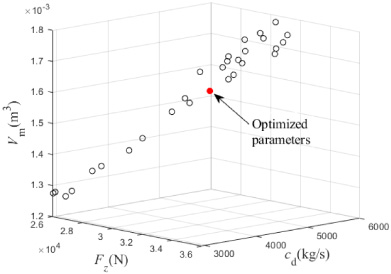
Pareto optimal front of the optimization result.

Fig. 23.

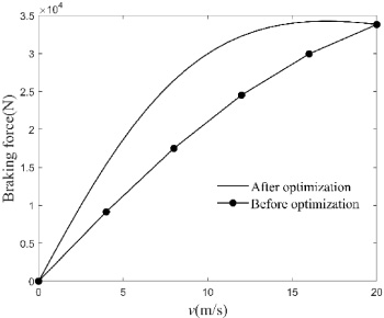
Braking force characteristics before and after optimization.

Table 4

Optimization results

Parameter	Initial	After optimization			Difference (%)
b (mm)	20		12.6		−37.0
c (mm)	20		32.6		63.0
d (mm)	1		1.9		90.0
h _m (mm)	20		16.5		−17.5
V _m (cm³)	1779.4		1642.4		−7.7
DD (kg ⋅ cm⁻³⋅ s⁻¹)	1.3		2.48		90.8
FD (kg ⋅ cm⁻²⋅ s⁻²)	14.63		20.14		37.7
		FEM	BP	Error
F _z (N)	26032	33071	32734	1.02%	27
c _d (kg ⋅ s⁻¹)	2314.1	4072.4	4069.3	0.08%	76

In such devices, the radial and axial components of the Lorentz force are very high. Thus these forces should be considered [28,29]. After the optimization of the ECB in this paper, the overall braking force characteristics have been improved. At the same time, it is necessary to ensure that the mechanical strength of the optimized ECB meets the requirements of use. Using the COMSOL Multiphysics software, the AC/DC module and the structural mechanics module are coupled to calculate the stress distribution of the ECB. The material properties of conductive tube and back iron used in ECB are presented in Table 5. The axial force density and radial force density distribution of the conductive tube are shown in the Fig. 24. The conductive tube and the back iron are interference fit, and the interference is 0.4 mm. The coefficient of friction between the two is 0.17. The stress distribution of the inner tube is shown in Fig. 25. The maximum stress is less than the yield stress, so the optimized ECB is safe.

Table 5

Material properties of conductive tube and back iron

	Poisson ration	Density (kg/m³)	Young’s modulus (GPa)	Yield stress (MPa)
Conductive tube (6061-T6)	0.33	2800	70	255
Back iron (1045)	0.30	7800	210	320

Fig. 24.

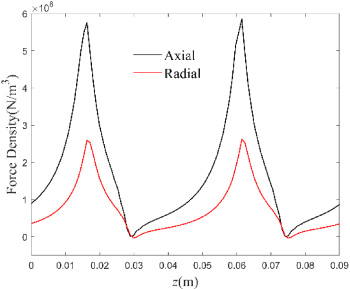
The axial force and radial force density distribution of the conductive tube.

Fig. 25.

The stress distribution at the end of the conductive tube.

4. Conclusion

Based on the Fourier series and the method of separating variables, an analytical model in a cylindrical coordinate system is established in this paper. The results of the analytical model are in good agreement with the results of the finite element method. Through harmonic analysis, it can be found that the error of braking force is only 0.083% by calculating only the first, fifth and ninth order harmonics. A multi-objective optimization design of eddy current brake is carried out by combining BP neural network surrogate model and GA. After optimization, the braking force of the eddy current brake increased by 27%, the damping coefficient increased by 76%, and the volume of the permanent magnet decreased by 7.7%.

Footnotes

Acknowledgements

This work was supported by the National Natural Science Foundation of China under Project 11572158 and 51705253, and the Postgraduate Research & Practice Innovation Program of Jiangsu Province under Grant KYCX19_0334.

Appendix

The expressions of constants $\text{C}_{n}^{\text{IV}}$ and $\text{D}_{n}^{\text{IV}}$ are presented by (A.1) $\begin{eqnarray}\displaystyle \text{} & \text{} & \displaystyle \text{C}_{n}^{\text{IV}}=-{\displaystyle \frac{\text{S}_{1}\text{O}_{5}\text{Q}_{1}}{2\text{O}_{6}\text{Q}_{2}}}\end{eqnarray}$ (A.2) $\begin{eqnarray}\displaystyle \text{} & \text{} & \displaystyle \text{D}_{n}^{\text{IV}}=-\frac{\text{S}_{5}\text{O}_{5}\text{Q}_{1}}{2\text{O}_{6}\text{Q}_{2}}\end{eqnarray}$ where (A.3) $\begin{eqnarray}\displaystyle \text{} & \text{} & \displaystyle \text{Q}_{1}=(\text{U}_{1}+\text{U}_{2}+\text{U}_{3})\text{I}_{1}({\alpha}_{0})+(\text{U}_{4}+\text{U}_{5})\text{K}_{1}({\alpha}_{0})\end{eqnarray}$ (A.4) $\begin{eqnarray}\displaystyle \text{} & \text{} & \displaystyle \text{Q}_{2}=(\text{U}_{6}+\text{U}_{7})\text{I}_{1}({\alpha}_{0})+(\text{U}_{8}+\text{U}_{9})\text{K}_{1}({\alpha}_{0})\end{eqnarray}$ (A.5) $\begin{eqnarray}\displaystyle \text{} & \text{} & \displaystyle \text{U}_{1}=\text{K}_{0}({\alpha}_{1})\text{S}_{2}\text{I}_{1}({\alpha}_{1})\end{eqnarray}$ (A.6) $\begin{eqnarray}\displaystyle \text{} & \text{} & \displaystyle \text{U}_{2}=({\mu}_{5}\text{S}_{2}\text{I}_{0}({\alpha}_{1})-({\mu}_{5}-1)\text{S}_{4}\text{K}_{0}({\alpha}_{1})-{\mu}_{5}\text{S}_{3}\text{O}_{6})\text{K}_{1}({\alpha}_{1})\end{eqnarray}$ (A.7) $\begin{eqnarray}\displaystyle \text{} & \text{} & \displaystyle \text{U}_{3}=-j{\pi}B_{resr}^{n}\text{K}_{0}({\alpha}_{1})\text{O}_{6}\text{L}_{1}({\alpha}_{1})\end{eqnarray}$ (A.8) $\begin{eqnarray}\displaystyle \text{} & \text{} & \displaystyle \text{U}_{4}=((1-{\mu}_{5})\text{S}_{2}\text{I}_{0}({\alpha}_{1})+{\mu}_{5}(\text{S}_{4}\text{K}_{0}({\alpha}_{1})+\text{S}_{3}\text{O}_{6}))\text{I}_{1}({\alpha}_{1})\end{eqnarray}$ (A.9) $\begin{eqnarray}\displaystyle \text{} & \text{} & \displaystyle \text{U}_{5}=(\text{S}_{4}\text{K}_{1}({\alpha}_{1})-j{\pi}B_{resr}^{n}\text{O}_{6}\text{L}_{1}({\alpha}_{1}))\text{I}_{0}({\alpha}_{1})\end{eqnarray}$ (A.10) $\begin{eqnarray}\displaystyle \text{} & \text{} & \displaystyle \text{U}_{6}=(\text{W}_{1}+\text{W}_{2})\text{K}_{0}({\alpha}_{1})\text{I}_{1}({\alpha}_{1})\end{eqnarray}$ (A.11) $\begin{eqnarray}\displaystyle \text{} & \text{} & \displaystyle \text{U}_{7}=[{\mu}_{5}(\text{W}_{1}+\text{W}_{2})\text{I}_{0}({\alpha}_{1})-({\mu}_{5}-1)(\text{W}_{3}+\text{W}_{4})\text{K}_{0}({\alpha}_{1})]\text{K}_{1}({\alpha}_{1})\end{eqnarray}$ (A.12) $\begin{eqnarray}\displaystyle \text{} & \text{} & \displaystyle \text{U}_{8}=[(1-{\mu}_{5})(\text{W}_{1}+\text{W}_{2})\text{I}_{0}({\alpha}_{1})+{\mu}_{5}(\text{W}_{3}+\text{W}_{4})\text{K}_{0}({\alpha}_{1})]\text{I}_{1}({\alpha}_{1})\end{eqnarray}$ (A.13) $\begin{eqnarray}\displaystyle \text{} & \text{} & \displaystyle \text{U}_{9}=(\text{W}_{3}+\text{W}_{4})\text{I}_{0}({\alpha}_{1})\text{K}_{1}({\alpha}_{1})\end{eqnarray}$ (A.14) $\begin{eqnarray}\displaystyle \text{} & \text{} & \displaystyle \text{S}_{1}=-m^{\prime }{\mu}_{5}\text{K}_{0}({\beta}_{4})\text{K}_{1}({\alpha}_{4})+m\text{K}_{0}({\alpha}_{4})\text{K}_{1}({\beta}_{4})\end{eqnarray}$ (A.15) $\begin{eqnarray} \displaystyle \text{} & \text{} & \displaystyle \text{S}_{2}=[2B_{resz}^{n}+j{\pi}B_{resr}^{n}\text{L}_{0}({\alpha}_{2})]\text{K}_{1}({\alpha}_{2}) + j{\pi}B_{resr}^{n}\text{L}_{1}({\alpha}_{2})\text{K}_{0}({\alpha}_{2}) \end{eqnarray}$ (A.16) $\begin{eqnarray}\displaystyle \text{} & \text{} & \displaystyle \text{S}_{3}=j{\pi}B_{resr}^{n}\text{L}_{0}({\alpha}_{1})+2B_{resz}^{n}\end{eqnarray}$ (A.17) $\begin{eqnarray} \displaystyle \text{} & \text{} & \displaystyle \text{S}_{4}=[-2B_{resz}^{n}-j{\pi}B_{resr}^{n}\text{L}_{0}({\alpha}_{2})]\text{I}_{1}({\alpha}_{2}) + j{\pi}B_{resr}^{n}\text{L}_{1}({\alpha}_{2})\text{I}_{0}({\alpha}_{2}) \end{eqnarray}$ (A.18) $\begin{eqnarray}\displaystyle \text{} & \text{} & \displaystyle \text{S}_{5}=m^{\prime }{\mu}_{5}\text{I}_{0}({\beta}_{4})\text{K}_{1}({\alpha}_{4})+m\text{I}_{1}({\beta}_{4})\text{K}_{0}({\alpha}_{4})\end{eqnarray}$ (A.19) $\begin{eqnarray}\displaystyle \text{} & \text{} & \displaystyle \text{W}_{1}=-m^{\prime }{\mu}_{5}\text{K}_{1}({\alpha}_{4})\left[m^{\prime }\text{K}_{1}({\alpha}_{3})\text{O}_{1}+m\text{K}_{0}({\alpha}_{3})\text{O}_{2}\right]\end{eqnarray}$ (A.20) $\begin{eqnarray}\displaystyle \text{} & \text{} & \displaystyle \text{W}_{2}=m\text{K}_{0}({\alpha}_{4})[m^{\prime }\text{K}_{1}({\alpha}_{3})\text{O}_{3}+m\text{K}_{0}({\alpha}_{3})\text{O}_{4}]\end{eqnarray}$ (A.21) $\begin{eqnarray}\displaystyle \text{} & \text{} & \displaystyle \text{W}_{3}=-m^{\prime }{\mu}_{5}\text{K}_{1}({\alpha}_{4})[-m^{\prime }\text{I}_{1}({\alpha}_{3})\text{O}_{1}+m\text{I}_{0}({\alpha}_{3})\text{O}_{2}]\end{eqnarray}$ (A.22) $\begin{eqnarray}\displaystyle \text{} & \text{} & \displaystyle \text{W}_{4}=m\text{K}_{0}({\alpha}_{4})[-m^{\prime }\text{I}_{1}({\alpha}_{3})\text{O}_{3}+m\text{I}_{0}({\alpha}_{3})\text{O}_{4}]\end{eqnarray}$ (A.23) $\begin{eqnarray}\displaystyle \text{} & \text{} & \displaystyle \text{O}_{1}=\text{I}_{0}({\beta}_{3})\text{K}_{0}({\beta}_{4})-\text{I}_{0}({\beta}_{4})\text{K}_{0}({\beta}_{3})\end{eqnarray}$ (A.24) $\begin{eqnarray}\displaystyle \text{} & \text{} & \displaystyle \text{O}_{2}=\text{I}_{0}({\beta}_{4})\text{K}_{1}({\beta}_{3})+\text{I}_{1}({\beta}_{3})\text{K}_{0}({\beta}_{4})\end{eqnarray}$ (A.25) $\begin{eqnarray}\displaystyle \text{} & \text{} & \displaystyle \text{O}_{3}=\text{I}_{0}({\beta}_{3})\text{K}_{1}({\beta}_{4})+\text{I}_{1}({\beta}_{4})\text{K}_{0}({\beta}_{3})\end{eqnarray}$ (A.26) $\begin{eqnarray}\displaystyle \text{} & \text{} & \displaystyle \text{O}_{4}=\text{I}_{1}({\beta}_{3})\text{K}_{1}({\beta}_{4})-\text{I}_{1}({\beta}_{4})\text{K}_{1}({\beta}_{3})\end{eqnarray}$ (A.27) $\begin{eqnarray}\displaystyle \text{} & \text{} & \displaystyle \text{O}_{5}=\text{I}_{0}({\alpha}_{3})\text{K}_{1}({\alpha}_{3})+\text{I}_{1}({\alpha}_{3})\text{K}_{0}({\alpha}_{3})\end{eqnarray}$ (A.28) $\begin{eqnarray}\displaystyle \text{} & \text{} & \displaystyle \text{O}_{6}=\text{I}_{0}({\alpha}_{2})\text{K}_{1}({\alpha}_{2})+\text{I}_{1}({\alpha}_{2})\text{K}_{0}({\alpha}_{2})\end{eqnarray}$ $m^{\prime }=\sqrt{m}\sqrt{j{\mu}_{0}{\sigma}v+m}$ , 𝛼₀ = mr ₀, 𝛼₁ = mr ₁, 𝛼₂ = mr ₂, 𝛼₃ = mr ₃, 𝛼₄ = mr ₄, 𝛽₃ = m ^′ r ₃, 𝛽₄ = m ^′ r ₄.

References

Tarvirdilu Asl

YÜKsel

H.M.

and Keysan

, Multi-objective design optimization of a permanent magnet axial flux eddy current brake, Turk. J. Elec. Eng. Comp. Sci. 27 (2019), 998–1011.

Liang

Liu

and Liu

, Performance analysis and test of a novel eddy-current braking & heating system for electric bus, Energy Convers. Manage. 183 (2019), 440–449.

Wang

P.J.

and Chiueh

S.J.

, Analysis of eddy-current brakes for high speed railway, IEEE Trans. Magn. 34(4) (1998), 1237–1239.

Ebrahimi

Bolandhemmat

Khamesee

M.B.

and Golnaraghi

, A hybrid electromagnetic shock absorber for active vehicle suspension systems, Vehicle Syst. Dyn. 49(1) (2011), 311–332.

Guo

and Ye

, A model of magnetic field and braking torque in liquid-cooled permanent-magnet retarder accounting for the skin effect on permeability, IEEE Trans. Veh. Technol. 68(11) (2019), 10618–10626.

Cho

Liu

H.-C.

Ahn

Lee

and Lee

H.-W.

, Eddy current brake with a two-layer structure: Calculation and characterization of braking performance, IEEE Trans. Magn. 53(11) (2017), 1–5.

Sharif

Faiz

and Sharif

, Performance analysis of a cylindrical eddy current brake, IET Electric Power App. 6(9) (2012), 661–668.

Srivastava

R.K.

and Kumar

, An alternative approach for calculation of braking force of an eddy-current brake, IEEE Trans. Magn. 45(1) (2009), 150–154.

Lubin

and Rezzoug

, Steady-state and transient performance of axial-field eddy-current coupling, IEEE Trans. Ind. Electron. 62(4) (2015), 2287–2296.

10.

Amjadian

and Agrawal

A.K.

, A passive electromagnetic eddy current friction damper (PEMECFD): Theoretical and analytical modeling, Struct. Control Health Monit. 24(10) (2017), 1978–2001.

11.

Choi

J.-Y.

and Jang

S.-M.

, Analytical magnetic torque calculations and experimental testing of radial flux permanent magnet-type eddy current brakes, J. Appl. Phys. 111(7) (2012).

12.

Kou

Jin

Zhang

and Zhang

, Characteristic analysis and control of a hybrid excitation linear eddy current brake, Energies 8(7) (2015), 7441–7464.

13.

Yazdanpanah

and Mirsalim

, Analytical study of axial-flux hybrid excitation eddy current brakes, Int. J. App. Electromagn. Mech. 47(4) (2015), 885–896.

14.

Jin

Kou

Pan

and Song

, Analytical model for a permanent magnet eddy-current brake with transverse edge effect, IEEE Access 7 (2019), 61170–61179.

15.

Bae

J.-S.

Hwang

J.-H.

Park

J.-S.

and Kwag

D.-G.

, Modeling and experiments on eddy current damping caused by a permanent magnet in a conductive tube, J. Mech. Sci. Technol. 23(11) (2010), 3024–3035.

16.

Ebrahimi

Khamesee

M.B.

and Golnaraghi

, Eddy current damper feasibility in automobile suspension: Modeling, simulation and testing, Smart Mater. Struct. 18(1) (2009), 15017–15031.

17.

Wang

Jewell

G.W.

and Howe

, A general framework for the analysis and design of tubular linear permanent magnet machines, IEEE Trans. Magn. 35(3) (1999), 1986–2000.

18.

Bianchi

, Analytical field computation of a tubular permanent-magnet linear motor, IEEE Trans. Magn. 36(5) (2000), 3798–3801.

19.

Park

M.-G.

Choi

J.-Y.

Shin

H.-J.

Lee

and Hong

, Electromagnetic analysis and experimental testing of a tubular linear synchronous machine with a double-sided axially magnetized permanent magnet mover and coreless stator windings by using semianalytical techniques, IEEE Trans. Magn. 50(11) (2014), 1–4.

20.

Amara

Wang

and Howe

, Analytical prediction of eddy-current loss in modular tubular permanent-magnet machines, IEEE Trans. Energy Convers. 20(4) (2005), 761–770.

21.

Atallah

Zhu

Z.Q.

Howe

and Birch

T.S.

, Armature reaction field and winding inductances of slotless permanent-magnet brushless machines, IEEE Trans. Magn. 34(5) (1998), 3737–3744.

22.

Kou

Jin

Zhang

and Zhang

, Modeling and analysis of force characteristics for hybrid excitation linear eddy current brake, IEEE Trans. Magn. 50(11) (2014), 1–5.

23.

Yang

Zhou

Zhu

Tang

and Wang

, Linear permanent magnet eddy current brake for overwinding protection, IEEE Access 7 (2019), 33922–33931.

24.

Shin

H.-J.

Choi

J.-Y.

Cho

H.-W.

and Jang

S.-M.

, Analytical torque calculations and experimental testing of permanent magnet axial eddy current brake, IEEE Trans. Magn. 49(7) (2013), 4152–4155.

25.

Canova

and Vusini

, Analytical modeling of rotating eddy-current couplers, IEEE Trans. Magn. 41(1) (2005), 24–35.

26.

Weise

Carlstedt

Ziolkowski

Brauer

and Toepfer

, Lorentz force on permanent magnet rings by moving electrical conductors, IEEE Trans. Ind. Electron. 51(12) (2015), 1–11.

27.

Gysen

B.L.J.

Meessen

K.J.

Paulides

J.J.H.

and Lomonova

E.A.

, General formulation of the electromagnetic field distribution in machines and devices using fourier analysis, IEEE Trans. Magn. 46(1) (2010), 39–52.

28.

Ebrahimi

B.M.

Saffari

Faiz

and Fereidunian

, Analytical estimation of short circuit axial and radial forces on power transformers windings, IET Gener. Transm. Distrib. 8(2) (2014), 250–260.

29.

Moradnouri

Vakilian

Hekmati

and Fardmanesh

, Optimal design of flux diverter using genetic algorithm for axial short circuit force reduction in HTS transformers, IEEE T. Appl. Supercon. 30(1) (2020).