Control-oriented modeling for the electrodynamic levitation with permanent magnet Halbach array

Abstract

Poor stability of the permanent magnet electrodynamic levitation hinders its application in the maglev field. Therefore, building a control-oriented model to improve its stability is most challenging. However, intractable electromagnetic models leading to an implicit relationship between levitation force and gap, yields a barrier for model-based controller design. To solve the above-mentioned problem, this paper develops a control-oriented model by two stages. Specifically, the first stage is to show an explicit formula of the levitation force with regard to the levitation gap by neglecting end effect; meanwhile the “maximum–minimum rectification” method is put forward to evaluating an accurate levitation force. The second stage is to bring forth the control-oriented model on basis of the estimated levitation force. Although the paper focus mainly on the development of the control-oriented model, an example of PD controller is provided to verify its validation. Experiment results demonstrate the estimated levitation force is highly consistent with the real one. Simulation results show that the control-oriented model is sufficiently reliable. The research bridges the gap between the physical model and the model-based controller for the electrodynamic levitation with permanent magnet Halbach array.

Keywords

Electrodynamic levitation Halbach array control-oriented levitation force

1. Introduction

Electrodynamic levitation technique has been applied for many domains, such as maglev train, maglev flywheel, electromagnetic braking and magnetic coupling. Especially, recent successful application of the technique in the Hyperloop pod test, reached a high speed of 463 km/h. It indicates a high potential application for permanent electrodynamic levitation in the ultra-high-speed ground transportation. Electrodynamic levitation has an advantage of large levitation gap over the electromagnetic levitation. However, much work needs to be done to solve exist problems, such as coupling between the mechanical motion and electromagnetic field, optimizing of the Halbach array structure and its stability. To solve these problems, explicit and accurate levitation force expression is urgent.

For an ideal Halbach array, its magnetic field mainly concentrates in the front and is weak in the back. Due to the excellent performance of the Halbach array, as well as for safety and economy prospects, electrodynamic levitation with permanent magnet Halbach array was adopted by GA Urban maglev [1] and Magplane [2]. It indicates the electrodynamic levitation has the potential to apply in the maglev traffic in the future. Problems like the structure optimization and the oscillation depression have been focused by researchers. The purpose of the structural optimization is to produce enough levitation force at the least expense of permanent magnets. Meanwhile, the latter one is to make the levitation gap stable at a certain working point. The article will deal with the latter problem. The key to solve the above problems is to clarify the mapping between the levitation force and parameters including the levitation gap, Halbach array sizes and horizontal speed.

Generally, the analytic method and numerical method can both be used to compute levitation force. Analytical method divides the whole regions into eddy current filed region and none-eddy current field region. By establishing electromagnetic field vector and potential function differential equations in different regions, governing equations can be solved under boundary conditions. The levitation force can be derived by Lorentz force formula or Maxwell stress tensor method. Reference [3] built a 2D analytical model and showed that the magnetic force formula should be rectified by a given function to match the 3D finite element analysis result. The second-order vector potential method was used to build the 3D analytical model to analyze one-side and double-side linear motions of permanent magnet electrodynamic levitation [4,5]. Separation of variables method was also used to analyze the electromagnetic forces with back iron attached to conductor plate and permanent magnet Halbach array for linear motion [6] and rotary motion [7,8], confirming the accuracy of the 3D electromagnetic model. Though literature work claimed that the analytical result could match well with that of the finite element analysis or experiment, they did not show an explicit relationship between the levitation force and gap that could be used for the model-based control.

Besides, unlike modeling directly by electromagnetic field equations, scaling laws of the permanent magnet Halbach array electrodynamic suspension showed a reliable ratio of levitation force to the magnetic reluctance force [9]. Unfortunately, the levitation force expression had unknown parameters, leading to its restriction on the application of model-based control.

Highly similarity was shown in Refs [10–14] that the levitation force would rise up more and more slowly along with the increasing moving speed. Therefore, it can be deduced that when the moving speed is sufficient large, the levitation force would keep unchanged. It indicates the electrodynamic levitation may be a promising choice for high-speed transportation.

Numerical methods of calculating the electromagnetic field generally include moment method, finite element method, boundary element method and time domain finite difference method. Finite element method has been widely used to calculated the eddy current field strongly coupled with the mechanical motion for the transient model of the electrodynamic suspension [15–17]. Electromagnetic force obtained by the finite element method is more accurate than that by analytical methods. Yet, the finite element method cannot show the explicit relation between the levitation force and gap, and cannot directly be used for model-based control either.

Electrodynamic suspension is unstable and thus needs an active control [18–20]. Methods were put forward to improve its stability but not based on a control-oriented model [21–26]. However, without a control-oriented model, the corresponding controller design is difficult. On the one hand, levitation force obtained by the analytic and finite element methods in literature researches could not be directly used for model-based control. On the other hand, benefit from the advanced control theory and intelligent control algorithm, control-oriented modeling for the electrodynamic levitation with permanent magnet Halbach array is necessary to introduce advanced intelligent control method.

Based on the above observation, the aim of the article is to provides an accurate control-oriented model for controller design of the electrodynamic levitation with permanent magnet Halbach array. We firstly try to explore an explicit expression for levitation force by solving magnetic vector potential differential equations. Then we put forward the “maximum–minimum rectification” method to evaluate an accurate levitation force and obtain a control-oriented model.

The remainder of this paper is organized as follows. Section 2 shows the explicit expression of the levitation force by simplifying the physical model by neglecting the end effect. Section 3 puts forward the “maximum–minimum rectification” method to acquire an accurate electrodynamic levitation force, and shows an experiment to verify its correctness. Section 4 verifies the validation of the control-oriented model, based on the PD controller for Matlab Simulink and COMSOL with feedback built-in. Section 5 concludes the paper.

2. Electromagnetic modeling of the electrodynamic suspension

In this section, the permanent magnet Halbach array moving over a copper or aluminum plate was studied. The system is assumed stable in the vertical direction and moving over a constant speed in the horizontal direction. For avoiding intricate Fourier series expansion, the ideal permanent magnet Halbach array is firstly chosen as the research object, and the magnetization direction is supposed to be continuously changed. The whole solution space could be divided into four regions as shown in Fig. 1. Region I and III, filled with air, are static magnetic field domains. Region II is filled with ideal Halbach array. The magnetizing current model is used to represent the permanent magnet behaviour. Region IV is an eddy current field domain. The eddy current is induced by the horizontal movement of the Halbach array.

Fig. 1.

Solution domains division for the whole space.

Due to the skin effect of the eddy current, a conductor plate far thicker than the skin depth δ can be replaced by an infinite thick one. As a result, the electrodynamic force could be evaluated by modeling on permanent magnet Halbach array moving over an infinite thick conductor plate. Let v be the moving speed along the z-axis and 𝜆 the wavelength of the Halbach array. The frequency of the induced eddy current field is described as [27] $\begin{eqnarray}{\omega}=kv,\end{eqnarray}$ (1) where $\begin{eqnarray}k=\frac{2{\rm\pi}}{{\lambda}}.\end{eqnarray}$ (2) Denoting μ and σ separately as the permeability and conductivity of the conductor plate, the skin depth is calculated by $\begin{eqnarray}{\delta}=\sqrt{\frac{2}{{\mu}{\sigma}{\omega}}}.\end{eqnarray}$ (3) Denoting the magnetic vector potential in region i (i = I, II, III, IV) as A ⁱ(i = I, II, III, IV), which has unique x component [27 ]: $\begin{eqnarray}A_{x}^{i}(y,z)=\text{Im}\{{\dot{A}}_{x}^{i}(y)e^{j(kz-{\omega}t)}\},\end{eqnarray}$ (4) then, in region I, it holds $\begin{eqnarray}\frac{\partial ^{2}A_{x}^{\mathbf{I}}(y,z)}{\partial y^{2}}+\frac{\partial ^{2}A_{x}^{\mathbf{I}}(y,z)}{\partial z^{2}}=0.\end{eqnarray}$ (5) For an ideal Halbach array, magnetizing currents distribute only on the surfaces. Meanwhile, the magnetizing currents insides region II do not exist (refer to Appendix). On the upper and lower surface of the ideal Halbach array, the magnetizing currents are $\begin{eqnarray}J_{x}(y,z)=\text{Im}\{\dot{J}_{x}(y)e^{j(kz-{\omega}t)}\},\end{eqnarray}$ (6) where, $\begin{eqnarray}\dot{J}_{x}(y_{1}+d)=\frac{Br}{{\mu}_{0}},\end{eqnarray}$ (7) and $\begin{eqnarray}\dot{J}_{x}(y_{1})=-\frac{Br}{{\mu}_{0}}.\end{eqnarray}$ (8) Then region II could be equivalent to a combination of two magnetizing currents boundaries with the air in between. In region II, as well as region III, free currents are absent, leading to $\begin{eqnarray}\frac{\partial ^{2}A_{x}^{\mathbf{II}}(y,z)}{\partial y^{2}}+\frac{\partial ^{2}A_{x}^{\mathbf{II}}(y,z)}{\partial z^{2}}=0,\end{eqnarray}$ (9) and $\begin{eqnarray}\frac{\partial ^{2}A_{x}^{\mathbf{III}}(y,z)}{\partial y^{2}}+\frac{\partial ^{2}A_{x}^{\mathbf{III}}(y,z)}{\partial z^{2}}=0.\end{eqnarray}$ (10) For region IV, eddy currents would be induced inside it and it holds that $\begin{eqnarray}\frac{\partial ^{2}A_{x}^{\mathbf{IV }}(y,z)}{\partial y^{2}}+\frac{\partial ^{2}A_{x}^{\mathbf{IV }}(y,z)}{\partial z^{2}}={\mu}{\sigma}\frac{\partial A_{x}^{\mathbf{IV }}(y,z)}{\partial t}.\end{eqnarray}$ (11) The boundary conditions are $\begin{eqnarray}\left\{\begin{array}{@{}l@{}}{\dot{A}}_{x}^{\mathbf{I}}(+\infty )=0\\[5.0pt] {\dot{A}}_{x}^{\mathbf{I}}(y_{1}+d)={\dot{A}}_{x}^{\mathbf{II}}(y_{1}+d)\\[5.0pt] \displaystyle -\frac{1}{{\mu}_{0}}\frac{\partial {\dot{A}}_{x}^{\mathbf{I}}(y_{1}+d)}{\partial y}-\left(-\frac{1}{{\mu}_{0}}\frac{\partial {\dot{A}}_{x}^{\mathbf{II}}(y_{1}+d)}{\partial y}\right)=-\frac{B_{r}}{{\mu}_{0}}\\[13.0pt] {\dot{A}}_{x}^{\mathbf{II}}(y_{1})={\dot{A}}_{x}^{\mathbf{III}}(y_{1})\\[5.0pt] \displaystyle -\frac{1}{{\mu}_{0}}\frac{\partial {\dot{A}}_{x}^{\mathbf{II}}(y_{1})}{\partial y}-\left(-\frac{1}{{\mu}_{0}}\frac{\partial {\dot{A}}_{x}^{\mathbf{III}}(y_{1})}{\partial y}\right)=\frac{B_{r}}{{\mu}_{0}}\\[13.0pt] {\dot{A}}_{x}^{\mathbf{III}}(0)={\dot{A}}_{x}^{\mathbf{IV }}(0)\\[5.0pt] \displaystyle -\frac{1}{{\mu}_{0}}\frac{\partial {\dot{A}}_{x}^{\mathbf{III}}(0)}{\partial y}-\left(-\frac{1}{{\mu}}\frac{\partial {\dot{A}}_{x}^{\mathbf{IV}}(0)}{\partial y}\right)=0\\[12.0pt] {\dot{A}}_{x}^{\mathbf{IV }}(-\infty )=0.\end{array}\right.\end{eqnarray}$ (12) Note that the permeability of the air μ₀ is equal to that of the conductor plate μ. Suppose magnetic vector potentials in each region has the form of $\begin{eqnarray}\left\{\begin{array}{@{}l@{}}{\dot{A}}_{x}^{\mathbf{I}}(y)=C_{0}e^{-ky}\\[5.0pt] {\dot{A}}_{x}^{\mathbf{II}}(y)=C_{1}e^{ky}+C_{2}e^{-ky}\\[5.0pt] {\dot{A}}_{x}^{\mathbf{III}}(y)=C_{3}e^{ky}+C_{4}e^{-ky}\\[5.0pt] {\dot{A}}_{x}^{\mathbf{IV }}(y)=C_{5}e^{qy},\end{array}\right.\end{eqnarray}$ (13) where, $\begin{eqnarray}q=\sqrt{\frac{k^{2}+\sqrt{k^{4}+{\mu}^{2}{\sigma}^{2}{\omega}^{2}}}{2}}-\frac{{\mu}{\sigma}{\omega}}{\sqrt{2\left(k^{2}+\sqrt{k^{4}+{\mu}^{2}{\sigma}^{2}{\omega}^{2}}\right)}}j,\end{eqnarray}$ (14) and C ₀ ∼ C ₅ are constants. Equation (13) can separately be verified to satisfy (5), (9), (10), (11) and the first and last boundary conditions in (12). Applying (13) in the remaining boundary conditions of (12) yields $\begin{eqnarray}\left\{\begin{array}{@{}l@{}}C_{0}e^{-k(y_{1}+d)}=C_{1}e^{k(y_{1}+d)}+C_{2}e^{-k(y_{1}+d)}\\[5.0pt] C_{0}ke^{-k(y_{1}+d)}+C_{1}ke^{k(y_{1}+d)}-C_{2}ke^{-k(y_{1}+d)}=-B_{r}\\[5.0pt] C_{1}e^{ky_{1}}+C_{2}e^{-ky_{1}}=C_{3}e^{ky_{1}}+C_{4}e^{-ky_{1}}\\[5.0pt] -C_{1}ke^{ky_{1}}+C_{2}ke^{-ky_{1}}=-C_{3}ke^{ky_{1}}+C_{4}ke^{-ky_{1}}+B_{r}\\[5.0pt] C_{5}=C_{3}+C_{4}\\[5.0pt] C_{5}q=C_{3}k-C_{4}k,\end{array}\right.\end{eqnarray}$ (15) which contains six unknown constants and six linear independent equations. The solution can be expressed as $\begin{eqnarray}\left\{\begin{array}{@{}l@{}}\displaystyle C_{0}=\frac{B_{r}}{2k}\left[(1-e^{-kd})e^{ky_{1}}+\frac{k-q}{k+q}e^{-ky_{1}}+e^{-kd}-e^{k(y_{1}+d)}\right]\\[10.5pt] \displaystyle C_{1}=-\frac{B_{r}}{2k}e^{-k(y_{1}+d)}\\[10.5pt] \displaystyle C_{2}=\frac{B_{r}}{2k}\left[(1-e^{-kd})e^{ky_{1}}+\frac{k-q}{k+q}e^{-ky_{1}}+e^{-kd}\right]\\[10.5pt] \displaystyle C_{3}=\frac{B_{r}}{2k}e^{-ky_{1}}(1-e^{-kd})\\[10.5pt] \displaystyle C_{4}=\frac{B_{r}}{2k}e^{-ky_{1}}\frac{k-q}{k+q}(1-e^{-kd})\\[10.5pt] \displaystyle C_{5}=\frac{B_{r}(1-e^{-kd})e^{-ky_{1}}}{q+k}.\end{array}\right.\end{eqnarray}$ (16) The magnetic induction intensity in the conductor plate is $\begin{eqnarray}B_{z}^{\mathbf{IV }}(y)=-\frac{\partial A_{x}^{\mathbf{IV }}(y)}{\partial z}=-qA_{x}^{\mathbf{IV }}(y).\end{eqnarray}$ (17) The induced electric field intensity in the conductor plate is $\begin{eqnarray}E_{x}^{\mathbf{IV }}(y)=-\frac{\partial A_{x}^{\mathbf{IV }}(y)}{\partial t}=j{\omega}A_{x}^{\mathbf{IV }}(y).\end{eqnarray}$ (18) The volume levitation force density in the conductor plate can be expressed as $\begin{eqnarray}f=-{\sigma}E_{x}^{\text{IV}}B_{z}^{\text{IV}}=-{\sigma}j{\omega}A^{\text{IV}}\cdot qA^{\text{IV}}.\end{eqnarray}$ (19) The average volume levitation force density in a period is $\begin{eqnarray}\overline{f}=-\frac{1}{2}{\sigma}\text{Re}[j{\omega}A_{x}^{\mathbf{IV }}(y)(qA_{x}^{\mathbf{IV }}(y))^{\ast }]=-\frac{1}{2}{\omega}{\sigma}b|C_{5}|^{2}e^{2ay}.\end{eqnarray}$ (20) Assume that the width of the Halbach array along the x-direction is w, then the levitation force of N wavelengths Halbach array is $\begin{eqnarray}\displaystyle \hspace{-18.0pt}F_{\mathit{ideal}}(y_{1}) & = & \displaystyle -N{\lambda}w\int _{-\infty }^{0}\overline{f}dy\nonumber\\ \displaystyle \displaystyle & = & \displaystyle \frac{N{\lambda}{\mu}w{\sigma}^{2}B_{r}^{2}(1-e^{-kd})^{2}}{4k^{2}}\frac{v^{2}}{\displaystyle \left(\sqrt{1+\frac{{\mu}^{2}{\sigma}^{2}v^{2}}{k^{2}}}+1\right)^{\frac{3}{2}}\left(\left(\sqrt{1+\frac{{\mu}^{2}{\sigma}^{2}v^{2}}{k^{2}}}+1\right)^{\frac{1}{2}}+\sqrt{2}\right)}e^{-2ky_{1}}.\nonumber\\ \displaystyle & & \displaystyle\end{eqnarray}$ (21) Equation (21) shows that levitation force consists of three parts: the first part is related to the structure and material, which is independent of the speed; the second part is determined by the moving speed, which is regulated by the driving system; the last part shows the definite exponential relationship between the levitation force and gap.

When v ≫ k∕(μσ), Eq. (21) could be simplified as $\begin{eqnarray}F_{\mathit{ideal}}(y_{1})=\frac{N{\lambda}wB_{r}^{2}(1-e^{-kd})^{2}}{4{\mu}}e^{-2ky_{1}},\end{eqnarray}$ (22) which indicates the levitation force tends to keep invariant as the moving speed increases. It shows the electrodynamic levitation system is suitable for the high-speed transportation. Furthermore, Eq. (22) also shows the levitation force has no relationship with conductivity of the conductor plate. Therefore, a cheap aluminum rail can be suitable for high-speed electrodynamic levitation.

For non-ideal Halbach array, magnetizing currents distribute discretely inside and continuously on the upper and lower surface along the z-axis when neglecting the end effect. Thus, when applying Fourier series expansion, magnetizing currents inside the Halbach array can be ignored. Assuming that the Halbach array contains M block of permanent magnets in a period, then magnetizing currents distributed on the upper surface in half a period can be expressed by $\begin{eqnarray}\displaystyle J_{x}(y_{1}+d,z)=\left\{\begin{array}{@{}l@{}}\displaystyle 0,z\in \left(0,\frac{{\lambda}}{2M}\right]\\[5.0pt] \displaystyle \frac{B_{r}}{{\mu}_{0}}\sin \frac{2{\rm\pi}}{M},z\in \left(\frac{{\lambda}}{2M},\frac{{\lambda}}{2M}+\frac{{\lambda}}{M}\right]\\[12.0pt] \displaystyle \frac{B_{r}}{{\mu}_{0}}\sin \left(2\cdot \frac{2{\rm\pi}}{M}\right),z\in \left(\frac{{\lambda}}{2M}+\frac{{\lambda}}{M},\frac{{\lambda}}{2M}+2\frac{{\lambda}}{M}\right]\\[9.0pt] \cdots \\[5.0pt] \displaystyle \frac{B_{r}}{{\mu}_{0}}\sin \left((p+1)\cdot \frac{2{\rm\pi}}{M}\right),z\in \left(\frac{{\lambda}}{2M}+p\frac{{\lambda}}{M},\frac{{\lambda}}{2M}+(p+1)\frac{{\lambda}}{M}\right]\\[9.0pt] \cdots \\[5.0pt] \displaystyle \frac{B_{r}}{{\mu}_{0}}\sin \left(\left(\frac{M}{2}-1\right)\cdot \frac{2{\rm\pi}}{M}\right),z\in \left(\frac{{\lambda}}{2M}+\left(\frac{M}{2}-2\right)\frac{{\lambda}}{M},\frac{{\lambda}}{2M}+\left(\frac{M}{2}-1\right)\frac{{\lambda}}{M}\right]\\[5.0pt] \displaystyle 0,z\in \left(\frac{{\lambda}}{2M}+\left(\frac{M}{2}-1\right)\frac{{\lambda}}{M},\frac{{\lambda}}{2}\right],\end{array}\right. & & \displaystyle\end{eqnarray}$ (23) where, p is an integer, and 0 ≤ p ≤ M∕2 − 2. Applying the half-range Fourier series expansion in half a period, Eq. (23) could be rewritten as $\begin{eqnarray}J_{x}(y_{1}+d,z)=\mathop{\sum }_{n=1}^{+\infty }c_{n}\sin \frac{2n{\rm\pi}z}{{\lambda}},\end{eqnarray}$ (24) where, $\begin{eqnarray}c_{n}=\frac{4}{{\lambda}}\int _{0}^{\frac{{\lambda}}{2}}M_{z}\sin \frac{2n{\rm\pi}z}{{\lambda}}dz.\end{eqnarray}$ (25) Dominance of the first harmonic component allows magnetizing currents be approximated by $\begin{eqnarray}\displaystyle \hspace{-10.0pt}J_{x}(y_{1}+d,z) & {\approx} & \displaystyle c_{1}\sin \frac{2{\rm\pi}z}{{\lambda}}\nonumber\\ \displaystyle & = & \displaystyle \frac{4}{{\lambda}}\int _{0}^{\frac{{\lambda}}{2}}M_{z}\sin \frac{2{\rm\pi}z}{{\lambda}}dz\sin \frac{2{\rm\pi}z}{{\lambda}}\nonumber\\ \displaystyle & = & \displaystyle \frac{4}{{\lambda}}\sin \frac{2{\rm\pi}z}{{\lambda}}\left(\int _{0}^{\frac{{\lambda}}{2M}}0\sin \frac{2{\rm\pi}z}{{\lambda}}dz+\int _{\frac{{\lambda}}{2M}}^{\frac{{\lambda}}{2M}+\frac{{\lambda}}{M}}\frac{B_{r}}{{\mu}_{0}}\sin \frac{2{\rm\pi}}{M}\sin \frac{2{\rm\pi}z}{{\lambda}}dz\right.\nonumber\\ \displaystyle \text{} & \text{} & \displaystyle \left.+\cdots \int _{\frac{{\lambda}}{2M}+p\frac{{\lambda}}{M}}^{\frac{{\lambda}}{2M}+(p+1)\frac{{\lambda}}{M}}\frac{B_{r}}{{\mu}_{0}}\sin (p+1)\frac{2{\rm\pi}}{M}\sin \frac{2{\rm\pi}z}{{\lambda}}dz+\cdots +\int _{\frac{{\lambda}}{2M}+\left(\frac{M}{2}-1\right)\frac{{\lambda}}{M}}^{\frac{{\lambda}}{2}}0\sin \frac{2{\rm\pi}z}{{\lambda}}dz\right)\nonumber\\ \displaystyle & = & \displaystyle \frac{B_{r}}{{\mu}_{0}{\rm\pi}}M\sin \frac{{\rm\pi}}{M}\sin kz\nonumber\\ \displaystyle & = & \displaystyle \text{Im}\left\{\frac{B_{r}}{{\mu}_{0}{\rm\pi}}M\sin \frac{{\rm\pi}}{M}e^{j(kz-{\omega}t)}\right\}.\end{eqnarray}$ (26) Thus, Eq. (7) will be replaced by $\begin{eqnarray}\dot{J}_{x}(y_{1}+d)=\frac{B_{r}}{{\mu}_{0}{\rm\pi}}M\sin \frac{{\rm\pi}}{M}.\end{eqnarray}$ (27) Similarly, Eq. (8) will be replaced by $\begin{eqnarray}\dot{J}_{x}(y_{1})=-\frac{B_{r}}{{\mu}_{0}{\rm\pi}}M\sin \frac{{\rm\pi}}{M}.\end{eqnarray}$ (28) Replacing B _r with $\frac{B_{r}}{{\rm\pi}}M\sin \frac{{\rm\pi}}{M}$ in Eqs (12), (15), (16) and (21) leads to the levitation force for the non-ideal Halbach array being expressed as $\begin{eqnarray}\displaystyle F(y_{1}) & = & \displaystyle \frac{N{\mu}w{\sigma}^{2}Br^{2}}{2{\rm\pi}k^{3}}\cdot M^{2}\sin ^{2}\frac{{\rm\pi}}{M}\cdot (1-e^{-kd})^{2}\nonumber\\ \displaystyle \text{} & \text{} & \displaystyle \cdot \frac{v^{2}}{\displaystyle \left(\sqrt{1+\frac{{\mu}^{2}{\sigma}^{2}v^{2}}{k^{2}}}+1\right)^{\frac{3}{2}}\left[\left(\sqrt{1+\frac{{\mu}^{2}{\sigma}^{2}v^{2}}{k^{2}}}+1\right)^{\frac{1}{2}}+\sqrt{2}\right]}e^{-2ky_{1}}.\end{eqnarray}$ (29)

3. Reconstruction for the levitation forces

Section 2 ignored the end effect of a non-ideal Halbach array, thus may cause a deviation from the real case. As a result, a rectification for the levitation force expression is necessary. This section is dedicated to proving that the normalized levitation forces, which features the trend of the levitation forces, have slight difference between the analytical and finite element method. Due to the high coincidence of the levitation forces’ trend, the “maximum–minimum rectification” method can be put forward to acquiring an accurate levitation force. Its correctness will be verified by an experiment. The section lays a foundation for obtaining a control-oriented model for the electrodynamic levitation with permanent magnet Halbach array.

3.1. Normalization of the levitation forces

The aim of the normalizing levitation forces is to compare the resemblance between levitation force curves obtained by the analytical method and the finite element method. Taking the analytical levitation force for example, suppose the levitation gap is limited to a certain range, then the levitation force reaches the maximum when the levitation gap takes the smallest value $y_{1}^{\text{min}}$ , while minimum when takes the largest value $y_{1}^{\text{max}}$ . The normalization is to map the maximum value $F(y_{1}^{\text{min}})$ to 1 and the minimum value $F(y_{1}^{\text{max}})$ to 0. Then, the levitation force F (y ₁) can linearly be mapped as $(F(y_{1})-F(y_{1}^{\text{min}}))/(F(y_{1}^{\text{max}})-F(y_{1}^{\text{min}}))$ . Similarly, the levitation force obtained by simulation is normalized in the same way.

3.2. Modelling by finite element method

To analyze the levitation force, a 2D simulation model was constructed by COMSOL Multiphysics software to approximate the real one by the finite element method. We separately choose π∕6, π∕4 and π∕2 as the interval magnetization direction for neighbor magnets in the Halbach array. Variation range of each parameter is shown in Table 1. Since the thickness of the conductor plate should be far larger than the skin depth of eddy currents, the depth of conductor plate is set to be 40 mm. To alleviate the end effect, three periods of Halbach array are chosen. The whole region is solved by the magnetic field interface using a stationary study. Note that the Lorentz term is exerted on the conductor plate by setting the velocity value. The mesh grid division, with an infinite element domain in the outer boundaries, is shown in Fig. 2. Eight boundary layers are set next to the upper surface of the conductor plate. The outermost square boundaries have zero tangential components of the magnetic potential. The mesh level of air region is set to be normal, while the Halbach array and conductor plate regions are refined by halving the element size parameters of the normal level. As a result, the minimum element mesh quality is 0.13 and the average one is up to 0.85. The station solver is set by default, except that the relative tolerance is set to be 0.01. By sweeping parameters of the levitation gap, the height, wavelength and moving speed of the Halbach array, sufficient data are acquired.

Table 1
Parameters of Halbach array—conductor model

Parameter Quantity (unit) Value

B _r Remanence of the permanent magnet (T) 1.285

M Magnets numbers per period of the Halbach array 4, 8, 12

μ₀ Permeability of the air (H/m) 4π × 10⁻⁷

μ Permeability of the aluminum (H/m) 4π × 10⁻⁷

𝛼 Conductivity of the aluminum (S/m) 3.82 × 10⁷

y ₁ Levitation gap (m) 0.005, 0.010, 0.015, 0.020, 0.025, 0.030

w Width of the Halbach and conductor plate (m) 0.05

d Height of the Halbach (m) 0.015, 0.02, 0.025

𝜆 Wavelength of the Halbach array (m) 0.2, 0.4, 0.6

h Height of the conductor plate (m) 0.04

v Moving speed of the Halbach array (m/s) 50, 100, 150

Parameter	Quantity (unit)	Value
B _r	Remanence of the permanent magnet (T)	1.285
M	Magnets numbers per period of the Halbach array	4, 8, 12
μ₀	Permeability of the air (H/m)	4π × 10⁻⁷
μ	Permeability of the aluminum (H/m)	4π × 10⁻⁷
𝛼	Conductivity of the aluminum (S/m)	3.82 × 10⁷
y ₁	Levitation gap (m)	0.005, 0.010, 0.015, 0.020, 0.025, 0.030
w	Width of the Halbach and conductor plate (m)	0.05
d	Height of the Halbach (m)	0.015, 0.02, 0.025
𝜆	Wavelength of the Halbach array (m)	0.2, 0.4, 0.6
h	Height of the conductor plate (m)	0.04
v	Moving speed of the Halbach array (m/s)	50, 100, 150

Fig. 2.

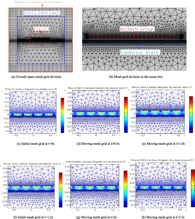
Mesh grid division for three period of Halbach array, comprised of eight magnets per period, moving over the conductor plate. Subgraph (a) shows an overview for the mesh grid of the stationary study; subgraph (b) shows the details inside the zoom box; subgraph (c)–(h) demonstrate the moving mesh technique by coupling the vertical movement with the finite element analysis for the time dependent study to obtain a dynamic simulation.

3.3. Normalized levitation forces comparison

Comparisons among normalized levitation forces under different gaps are shown in Fig. 3. Subgraph (a) shows the levitation force’s variation with gap under different magnetizing direction. Note that magnets numbers M per period of the Halbach array is chosen for convenient. It indicates that the magnetizing direction difference is 2π∕M between two neighboring magnets. For the magnetizing direction difference π∕2, π∕4 and π∕8, normalized levitation forces have an error less than 0.05 between the analytical and finite element methods. As the moving speed increases, the error changes little. It can be concluded that trends of levitation forces obtained by the analytical and finite element methods, are of highly resemblance. Impact of the wavelength on the trends’ similarity obtained by both methods, can be deduced from subgraph (b). The maximum error between the two methods is 0.13 under different wavelength. The moving speed has little impact on the error. So, trends of levitation forces acquired by the two methods are similar. The normalized levitation forces variation under different Halbach array heights is shown in subgraph (c). The maximum error is 0.02 with the levitation gap varying from 5 mm to 30 mm. The error varies little with the increase of the moving speed. For different Halbach array heights, high likeness is still kept between the analytical and finite element methods.

Fig. 3.

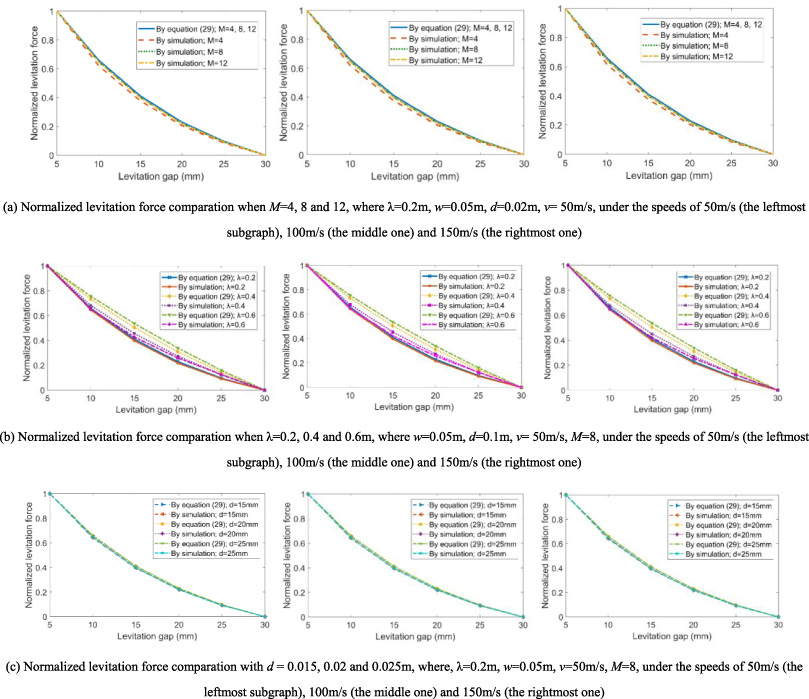
Normalized levitation forces comparation between the analytical method and the simulations; variation of the normalized levitation forces with levitation gap coincides well despite of different structural parameters under different speeds; subgraph (a) shows magnetizing directions little influence on the normalized levitation force coincidence; subgraph (b) indicates that for different wavelength, the normalized levitation forces are coincided; subgraph (c) demonstrates that the Halbach array height has little impact on the coincidence of the normalized levitation forces.

According to the above analysis, it can be concluded that levitation force trends, obtained by analytical and finite element methods, coincide well as levitation gap varies within a certain range despite of the structural parameters. Conversely, the high coincidence of the normalized levitation force could be used to deduce the accurate levitation force variation with levitation gap under different structural parameters.

3.4. Accurate levitation force estimation

Instead of fitting curves by acquiring so many points by experiment, two points are only needed to be acquired by experiment to estimate an accurate levitation force. According to the small difference between the normalized levitation force obtained by the two methods, the normalized levitation forces are deduced to be consistent for the analytical and experimental ones, that is $\begin{eqnarray} \frac{\overset{\frown}{F}(y_{1})-\overset{\frown}{F}(y_{1}^{\text{max}})}{\overset{\frown}{F}(y_{1}^{\text{min}})-\overset{\frown}{F}(y_{1}^{\text{max}})}=\frac{F(y_{1})-F(y_{1}^{\text{max}})}{F(y_{1}^{\text{min}})-F(y_{1}^{\text{max}})}, \end{eqnarray}$ (30) where, $\overset{\frown}{F}(y_{1}^{\text{min}})$ is the maximum value and $\overset{\frown}{F}(y_{1}^{\text{max}})$ the minimum value by experimental test. Taking ((29)) into ((30)), the “maximum–minimum rectification” is given to estimate accurate levitation force $\overset{\frown}{F}$ (y ₁) by $\begin{eqnarray} \overset{\frown}{F}(y_{1})={\kappa}_{1}e^{-2ky_{1}}-{\kappa}_{2}, \end{eqnarray}$ (31) where, $\begin{eqnarray} \displaystyle {\kappa}_{1} & = & \displaystyle \frac{N{\lambda}{\mu}w{\sigma}^{2}B_{r}^{2}(\overset{\frown}{F}(y_{1}^{\text{min}})-\overset{\frown}{F}(y_{1}^{\text{max}}))(1-e^{-kd})^{2}v^{2}}{\displaystyle 4k^{2}(F(y_{1}^{\text{min}})-F(y_{1}^{\text{max}}))\left(\sqrt{1+\frac{{\mu}^{2}{\sigma}^{2}v^{2}}{k^{2}}}+1\right)^{\frac{3}{2}}\left(\left(\sqrt{1+\frac{{\mu}^{2}{\sigma}^{2}v^{2}}{k^{2}}}+1\right)^{\frac{1}{2}}+\sqrt{2}\right)}, \end{eqnarray}$ (32) $\begin{eqnarray} \displaystyle {\kappa}_{2} & = & \displaystyle \frac{F(y_{1}^{\text{max}})}{F(y_{1}^{\text{min}})-F(y_{1}^{\text{max}})}(\overset{\frown}{F}(y_{1}^{\text{min}})-\overset{\frown}{F}(y_{1}^{\text{max}}))-\overset{\frown}{F}(y_{1}^{\text{max}}). \end{eqnarray}$ (33)

3.5. Experiment and verification

An existing rotating experimental device, as shown in Fig. 4, equipped with a block of permanent magnet Halbach array and an aluminum disk, is used to verify the effectiveness of the “maximum–minimum rectification” method. The Halbach array has a total length of 0.225 m and both the width and height are 0.04 m. The total length of the Halbach array is so smaller than the outermost perimeter of the disk that the rotary motion of the disk could be equivalent to a linear motion. The tray attached by the Halbach array could move freely along the sliders in the vertical direction by the support of a couple of linear bearings. Thus, force sensor I can be used to measure the lift force of the Halbach array. Force sensor II is used to measure the drag force. The radius of the aluminum disk is 0.35 m and the thickness is 30 mm. The permanent magnet Halbach array is 0.3 m away from the axis of the disk. When the disk is driven by the motor, the lift force of the permanent magnet Halbach array can be captured by the force sensor. The levitation force data are collected with the levitation gap being stable at 20 mm ∼ 35 mm. The estimated levitation force is also compared with the experimental one with the levitation gap increasing from 15 mm to 55 mm. Figure 5 shows that the estimated levitation force coincides well with the experimental one. Thus, the experiment proves that the “maximum–minimum rectification” method is validate.

Fig. 4.

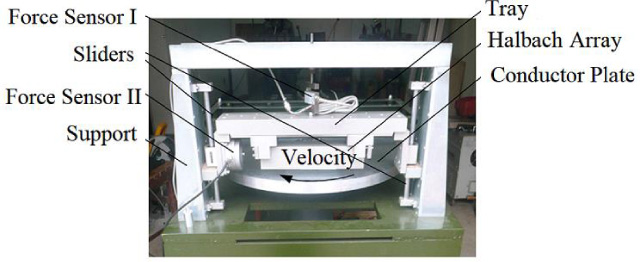
PM Halbach array—aluminum disk experimental device. The Halbach array is laid above the edge of the disk and the rotary motion of the disk could be equivalent to a linear motion; The tray attached by the Halbach array could move freely along the sliders in the vertical direction; Levitation force data can be acquired by force sensor I under different rotary speed and levitation gap. (For more details, refer to [28]).

Fig. 5.

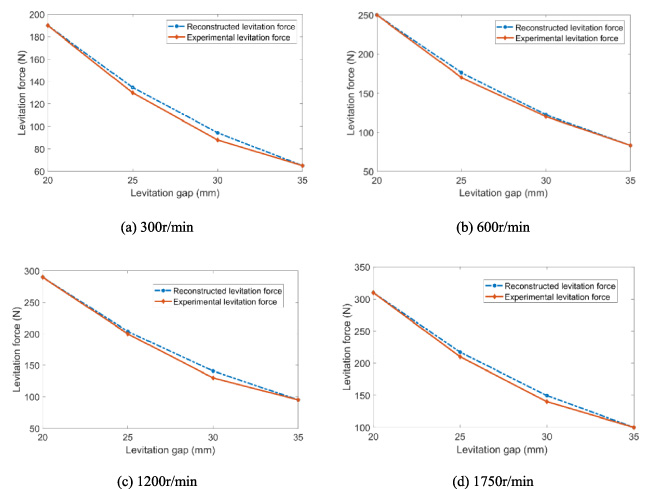
High accordance of the reconstructed levitation force with the experiment under different moving speed. The rotary speed is separately 300 r/min, 600 r/min, 1200 r/min, 1750 r/min; The levitation gap varies from 20 mm to 35 mm.

4. Control-oriented modelling and validation

Electrodynamic levitation is unstable without an active controller, as its damping is so weak that it would not be stable before a long-time vibration. Dynamic simulations have been done by both 2D numerical calculation using a moving mesh technique (refer to Fig. 2) with COMSOL finite element method (FEM) and Simulink in MATLAB software. The load is set to be 50 kg. The initial levitation gap is set to be 5 mm. Initial moving speed toward the vertical direction is set to be zero. Comparison shows dynamic response based on the control-oriented model is notably different from that of the finite element model after a few seconds (as shown in Fig. 6). The reason may be that the vertical movement coupled with the eddy current field yields a damping. However, at the beginning within 1 s, the two match so well. Imposing an active control at the initial time based on the estimated levitation force, the effect will be close to the real one.

Fig. 6.

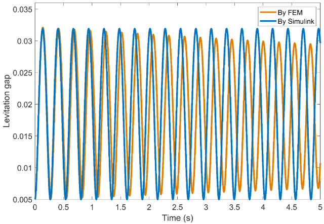
Levitation gap variation without control obtained by finite element method (FEM) and Simulink (where, 𝜆 = 0.24,w = 0.05 m, d = 0.02 m, y ₁ = 0.015 m, v = 50 m/s, M = 8).

Suppose the Halbach array is stable at a certain point, denoted as the working point, where the levitation force is equal to its load. An external force u, can be exerted on the Halbach array to realize the stability. Then the dynamic model of the electrodynamic levitation with permanent Halbach array is $\begin{eqnarray} m\ddot{y} _{1}=\overset{\frown}{F}(y_{1})-mg+u. \end{eqnarray}$ (34) At the working point y ₁ = y*, it holds $\begin{eqnarray} \overset{\frown}{F}(y^{\ast })-mg=0, \end{eqnarray}$ (35) which gives $\begin{eqnarray}{\kappa}_{1}e^{-2ky^{\ast }}-{\kappa}_{2}-mg=0.\end{eqnarray}$ (36) Inserting ((34)) and ((37)) into ((35)) gives the control-oriented model $\begin{eqnarray}\ddot{y} _{1}=\frac{{\kappa}_{1}}{m}e^{-2ky_{1}}-\frac{{\kappa}_{1}}{m}e^{-2ky^{\ast }}+\frac{u}{m}.\end{eqnarray}$ (37)

Considering practical projects using the PID or PD controller most for control, and the PD controller having an advantage of observing the steady-state error, the same PD controller is chosen for MATLAB Simulink and COMSOL FEM coupled with feedback. The PD controller is given by $\begin{eqnarray}u=K_{p}(y^{\ast }-y_{1})+K_{d}(0-{\dot{y}}_{1})+K_{i}\int _{0}^{t}(y^{\ast }-y_{1})dt.\end{eqnarray}$ (38)

To elaborate the effectiveness of verification method for the control-oriented model, we emphasize the difference between the two means:

(1) MATLAB Simulink builds block for the controlled object based on (34) and (37), but (34) is established at the premise of omitting the vertical movement. In practice, the vertical movement of the Halbach array would produce induced eddy currents always hindering the movement. A high-fidelity numerical simulation encompasses vertical damp can be chosen to reveal the fact.

(2) COMSOL FEM could realize the horizontal movement by setting up the Lorentz term and vertical movement by the moving mesh technique. Different from MATLAB Simulink, the feedback control is built-in by creating global differential equations to couple the movement with the eddy current field. By the backward differentiation method for time discretization and finite element method for space discretization, the full-coupled equations could be solved. In a word, the COMSOL FEM coupled with feedback control could realize a high-fidelity numerical simulation.

Dynamic response to the PD controller is separately simulated by MATLAB Simulink and COMSOL FEM. The initial value is set as former, and the working point is preset to be 10 mm. The proportional coefficient K _p is swept from 100000 to 50000 at a step size 5000 while differential coefficient K _d is set from 5000 to 9000 at a step size 500. Dynamic performances, including the rise time, peak time, overshoot and setting time, are compared in Fig. 7. Subgraph (a) shows the variation of the rise time with the proportional coefficient and differential coefficient. The maximum error between the simulink and the finite element method is only 0.01 s. Subgraph (b) demonstrates the peak time overlaps at some points, and the error between the two methods does not exceed than 0.007 s. Subgraph (c) presents that the overshoot obtained by simulink has only slight difference with that by finite element method, with an error less than 0.04%. Subgraph (d) displays the difference of the setting time between the two methods, and the error is within 0.04 s. Besides, the steady-state error between the two methods is below 0.07 mm given by Fig. 8. According to the results, it can be concluded that the control-oriented model is an accurate model and can directly be used for model-based controller design.

Fig. 7.

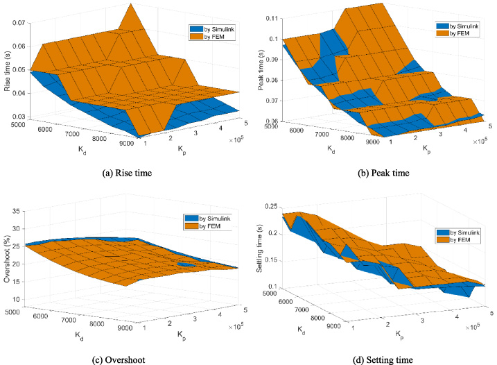
Comparison of dynamic performances for step response between the Simulink and the finite element method.

Fig. 8.

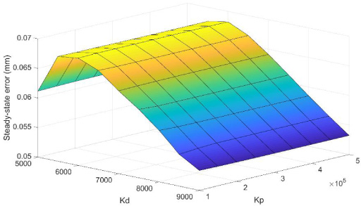
Steady-state errors between Simulink and FEM simulations.

5. Conclusion

This paper explored a control-oriented model for the electrodynamic levitation with permanent magnet Halbach array. By neglecting the end effect, an explicit levitation force formula has been given to clarify the mapping between the levitation force and levitation gap. Furthermore, the “maximum–minimum rectification” method is brought forth to evaluate the accurate levitation force; and experiment shows the validation of the method. The control-oriented model is put forward and justified by a PD controller with the proportional and differential coefficients varying over a large-scale range. The control-oriented model promises the well-established advance control theory, e.g. robust control, optimal control, etc. to be applied in the control of the electrodynamic levitation with permanent magnet Halbach array.

Footnotes

Proof of magnetizing currents being zero inside the ideal Halbach array

For the ideal Halbach array, it is regarded as uniformly and continuously magnetized. Then the magnetizing currents are seen as distributed on the front, rear, upper, lower surfaces. Note that the 2D analysis omitted the front and rear surfaces magnetizing currents. For any point at z, choose a microelement, with a width Δz and height d, neighboring to point z in region II, as shown in Fig. 9. At the interval [(z −Δz), z) and (z, (z + Δz)], the magnetization angles are separately θ −Δθ and θ + Δθ. At point z, the magnetizing current are expressed as (39) $\begin{eqnarray}\displaystyle j_{z} & = & \displaystyle \frac{B_{r}}{{\mu}_{0}}\sin ({\theta}-{\rm\Delta}{\theta})-\frac{B_{r}}{{\mu}_{0}}\sin ({\theta}+{\rm\Delta}{\theta})\nonumber\\ \displaystyle & = & \displaystyle -\frac{2B_{r}}{{\mu}_{0}}\cos {\theta}\sin ({\rm\Delta}{\theta}).\end{eqnarray}$ Note that θ has a linear relationship with z, so that when Δz → 0, Δθ → 0 and sin(Δθ) → 0. Meanwhile cosθ is a bounded value. Thus, j _z = 0 for any point z. That means magnetizing currents is zero inside the ideal Halbach array.

References

Gurol

Baldi

Jeter

Kim

I.K.

and Bever

, General atomics low speed maglev technology development program (supplemental #3), Magnetic Levitation Vehicles 57(10) (2005), 2988–3000.

Montgomery

D.B.

, Overview of the 2004 magplane design, Magplane Technology, Inc, Tech. Rep, 2004.

Wang

Lin

and Fang

, Analytical prediction of torque characteristics of Eddy current couplings having a Quasi-Halbach magnet structure, IEEE Transactions on Magnetics 52(6) (2015), 1–9.

Chen

Zhang

Bird

J.Z.

Paul

and Zhang

, A 3-D analytic-based model of a null-flux Halbach array electrodynamic suspension device, IEEE Transactions on Magnetics 51(11) (2015), 1–5.

Luo

Zhang

and Jing

, 3D analytical model of permanent magnet and electromagnetic hybrid Halbach array electrodynamic suspension system, Journal of Electrical Engineering & Technology 15(4) (2020), 1713–1721.

Tongyu

and Dazhi

, 3D Analytical model of drag and lift force for a conductive plate moving above a Halbach magnet array, Transactions of the Institute of Measurement and Control 40(12) (2018), 3515–3524.

Jin

Tian

Guo

and Zhu

, 3-D analytical magnetic field analysis of the Eddy current coupling with Halbach magnets, IEEE Transactions on Magnetics 56(1) (2020), 1–4.

Paul

and Bird

J.Z.

, Improved analytic model for eddy current force considering edge-effect of a conductive plate, in: XXII International Conference on Electrical Machines, 2016.

Flankl

Wellerdieck

Tüysüz

and Kolar

J.W.

, Scaling laws for electrodynamic suspension in high-speed transportation, IET Electric Power Applications 12(3) (2017), 357–364.

10.

Chaidez

Bhattacharyya

S.P.

and Karpetis

A.N.

, Levitation methods for use in the hyperloop high-speed transportation system, Energies 12 (2019).

11.

Abdelrahman

A.S.

, Hyperloop transportation system: Analysis, design, control, and implementation, IEEE Transactions on Industrial Electronics 65(9) (2018), 7427–7436.

12.

Iniguez

and Raposo

, Numerical simulation of a simple low-speed model for an electrodynamic levitation system based on a Halbach magnet array, Journal of Magnetism & Magnetic Materials 322(9-12) (2010), 1673–1676.

13.

Cho

H.W.

Han

H.S.

Bang

J.S.

Sung

H.K.

and Kim

B.H.

, Characteristic analysis of electrodynamic suspension device with permanent magnet Halbach array, Journal of Applied Physics 105(7) (2009), pt. 2, p. 08P510.

14.

Bird

and Lipo

T.A.

, Characteristics of an electrodynamic wheel using a 2-D steady-state model, IEEE Transactions on Magnetics 43(8) (2007), 3395–3405.

15.

Duan

Xiao

Zhang

Rotaru

and Sykulski

J.K.

, Analysis and optimization of asymmetrical double-sided electrodynamic suspension devices, IEEE Transactions on Magnetics 55(6) (2019), 1–5.

16.

Zhang

Wang

and Geng

, Design and optimization of Halbach-Array PM rotor for high-speed axial-flux permanent magnet machine with ironless stator, IEEE Transactions on Industrial Electronics 99 (2019), 1.

17.

Duan

Xiao

Zhang

Rotaru

and Sykulski

, Analysis and optimization of asymmetrical double-sided electrodynamic suspension devices, IEEE Transactions on Magnetics 55(6) (2019).

18.

Ham

Lin

K.C.

and Joo

, Study of a hybrid magnet array for an electrodynamic maglev control, Journal of Magnetics 18(3) (2013), 370–374.

19.

Long

and Xue

, Study of EDS & EMS hybrid suspension system with permanent-magnet Halbach array, IEEE Transactions on Magnetics 47(12) (2011), 4717–4724.

20.

Long

and Zhang

, Experimental research on an energy-saving maglev train, Environmental Engineering & Management Journal (EEMJ) 10(7) (2011).

21.

Boeij

J.D.

Steinbuch

and Gutierrez

H.M.

, Mathematical model of the 5-DOF sled dynamics of an electrodynamic maglev system with a passive sled, IEEE Transactions on Magnetics 41(1) (2005), 460–465.

22.

Boeij

J.D.

Steinbuch

and Gutierrez

, Real-time control of the 3-DOF sled dynamics of a null-flux maglev system with a passive sled, in: IEEE International Symposium on Industrial Electronics, 2006.

23.

Okubo

Ueda

and Ohashi

, Effective control method of the active damper system against the multidirectional vibration in the superconducting magnetically levitated bogie, IEEE Transactions on Applied Superconductivity 26(4) (2016), 1–4.

24.

Zhou

Kou

Wang

and Xing

, Modeling and analysis of a maglev vibration isolation unit using rectangle Halbach permanent magnet array, in: 2014 17th International Conference on Electrical Machines and Systems (ICEMS), 2014, pp. 1711–1714.

25.

Fang

and Sun

, Design of a Halbach array permanent magnet damping system for high speed compressor with large thrust load, IEEE Transactions on Magnetics 51(1) (2015), 1–9.

26.

Dynamic response characteristics of high temperature superconducting maglev systems: Comparison between Halbach-type and normal permanent magnet guideways, Physica C Superconductivity & its Applications 519 (2015), 147–152.

27.

Post

and Ryutov

, The Inductrack Concept: A New Approach to Magnetic Levitation, Livermore, CA, 1996, UCRL-ID-124115.

28.

Yuwei

, Technological Analysis for Permanent Magnet EDS System Based on Halbach Structure, 2009, (in Chinese).