
Abstract
In this article we present an approach to the quantitative evaluation of the 3D printed sample made of polyethylene terephthalate glycol (PETG) using the active infrared thermography (AIT) method with halogen lamps excitation. For this purpose, numerical and experimental studies were carried out. The numerical model solved with finite element method (FEM) was used first to create a database of signals and further to train neural networks. The networks were trained to detect the heterogeneity of the internal structure of the tested printed sample and to estimate the defects position. After training, the performance of the network was validated with the data obtained in the experiment carried out with the active thermography regime on a real 3D print identical to the modelled one.
Keywords
Introduction
3D printing, known also as additive manufacturing (AM), is now widely used in many industry branches. Initially, printed structures were used mainly in the design and creation of preliminary prototypes [1]. However, the development of 3D printing techniques caused that such structures are more and more often also the final product. The variety of materials currently available for use in AM makes printed elements appear in the advanced industries including, but not limited to, the medical (for building blood vessels or low-cost prosthetic parts), architectural, and automotive. Such use of these materials makes it important to assess their quality. Process control in AM is possible at all its stages—preparatory (examination of the quality of the feedstock material), print stage (control of the printing process), and the final evaluation of the finished product [2]. Herein, we focus on quality control in the final stage of 3D printing production.
In this article, one of the non-destructive testing techniques (NDT) - active infrared thermography (AIT) [3–6] was used to qualitative and quantitative assess of the printed structure, this approach is relatively new and has so far been published in only a few articles [7–9]. In this method, an external energy source is used to create a temperature difference within the test sample. This difference is observed on the sample’s surface using a thermal imaging camera. Heterogeneities inside the examined structure are visible as deviations (warmer or cooler spots) in the observed distribution.
The key goal of this work is the processing of the data obtained in a result of the thermovison inspection in order to qualitatively assess the tested 3D prints. Therefore the automatic defects recognition procedure, based on neural network (NN) models, was developed. The high efficiency of such procedure is highly dependent on the formulation of such post-processing procedures in the database that will enable unambiguous differentiation, often multi-threaded, dependencies between the object’s condition and the characteristics of the recorded infrared radiation. The use of a set of features for this purpose, indisputably characterizing a given signal, is often charged to a large error resulting from human participation (and thus subjective one) in such a process (e.g., through manual configuration or adaptation of parameterization procedures). Therefore, researchers are interested in relying on methods that allow this stage to be skipped in favour of automated procedures. Over the past decade, deep neural networks have gained importance in this area due to the ability to efficiently solve a very wide range of problems [7,8,10,11]. One of the key factors influencing the observed dynamics of deep learning development in many applications is the elimination of the need to manually parameterize the analysed phenomenon in order to conduct the behavioural learning process [8,12]. A special group in the context of the presented in this paper experiments and analysis (of the infrared radiation of the tested object with defects) are recursive RNN neural networks. These networks are the subject of many research works in a wide range of applications due to their enormous possibilities of modelling and predicting the dynamics of nonlinear time-varying systems [10,13]. RNNs are generally capable of creating and processing records of any sequence of input data. RNNs can learn rules and dependencies that combine sequential and parallel information processing in an efficient way based on mass parallelism. As a result, it enables the achievement of a significant decrease in computational costs. Recently, networks based on the Long Short-Term Memory (LSTM) mechanism stand out among recursive networks with a significant potential and achievements. Contrary to the regular RNN, in which there is a vanishing gradient effect, LSTM networks have a modified structure, thanks to which it is possible to capture multiple time dependencies with different characteristics, including long-term effects [10,13,14]. Therefore, considering that the defects occurring in the tested object have both a short-term and long-term effect on the characteristics of the obtained infrared radiation waveforms, a structure based on a unidirectional LSTM network was used to implement the final procedure of automatic defect recognition in the tested object.
In order to prepare the experiment, appropriate samples were printed and tested by means of active thermography with halogen lamps excitation. In the designed experiment, simple sample geometry (cuboid) and defects in the form of printed cylindrical holes of various diameters and depths were assumed. In the first stage, a numerical model representing real experimental conditions was prepared in the COMSOL environment. In the second stage, the prepared model was used to create a database that served as a training material for the designed LSTM network. The task of the trained network was to detect and localize the defects. The third step was the validation of the trained network on the experimental data. It should be emphasized that the application of numerical data to the trained network allows for the automation of the sample control process. According to the authors’ knowledge, the use of deep LSTM networks trained on numerical data to assess the condition of printed materials based on thermal imaging inspection has not been published so far.
Experimental methodology and numerical model
The main goal of this study was to develop a technique for the real samples evaluation, based on neural networks trained on the numerical data. This approach allows for the creation of a more general database and can be the basis for automating the process of assessing structures tested using the thermovision method. In order for the created database to be useful in this case, it is necessary to build a numerical model accurately reflecting the experimental scenario. In this section, the experimental setup, tested samples and assumptions of the numerical model are presented.
Evaluated sample and experimental setup
The tested sample was printed using the 3D printing technique utilizing the Filament Fuse Fabrication (FFF) method. The popular, durable and easy to print polyethylene terephthalate glycol (PETG) filament was used. The printout density has been set to 100%. The sample was designed as a flat plate, 105 ×105 ×7 mm in size with a series of holes of various diameters (1.4 to 7 mm) and depths (1.4 to 4.2 mm). The sample CAD model and a photo are presented in Fig. 1. Like most of the available filaments, PETG is a material with a low coefficient of thermal conductivity. Its basic thermal properties, important in the presented analysis, are summarized in the Table 1.
The basic heat properties of PETG
The basic heat properties of PETG

Experimental sample – CAD model and a photo of printed structure (dimensions in [mm]).
The material was tested with the active infrared thermography (AIT) with halogen lamp excitation. The transmission technique was used: the material was heated from the rear side (RS) and observed from the front side (FS). Due to the poor thermal conductivity of the tested material, long step heating was selected. The heating time was set to 60 s, followed by 300 s of natural cooling of the sample. Throughout this time, the temperature distribution on the front side of the sample was registered with a thermal imaging camera, and the recording frequency was 1 frame per second. As a result, 360 thermograms were obtained, ready for further processing. In Fig. 2 the experimental setup is presented.
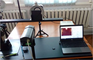
Experimental setup.
The numerical model was prepared with the commercial Finite Element Method based (FEM) COMSOL Multiphysics environment with Heat Transfer and Surface to Surface Radiation module, using the radiosity method to model the radiation on diffuse surfaces. Here we assume that the only heating mechanism in the system is the radiation. Therefore the most important factor is the heat flux by radiation, introduced at the heated surface. This expression is dependent on the two main variables: total irradiation and radiosity. The irradiation can be defined as the total incoming radiative flux, caused by the external energy sources, whereas the radiosity is the sum of diffusively reflected and emitted radiation:
The geometry of the system is presented in the Fig. 3. For the whole geometry simplification the heat source (a halogen lamp in the experiment) was simulated here as 33 point sources with a given power, radially distributed at a distance of 10 cm from the heated surface of the sample. To simulate the real life heat source the power given at a single point source was decaying in every row linearly from 100% in the centre to 20% at the outermost row. It will be further shown, that made assumptions did not have the significant impact on the time-temperature characteristics obtained as a result of the simulation. The location of the source is shown in the Fig. 3(a). As in the experiment, the transmission method was used, hence the temperature is measured on the front surface and the rear surface is heated, as shown in Fig. 3(b) and 3(c).
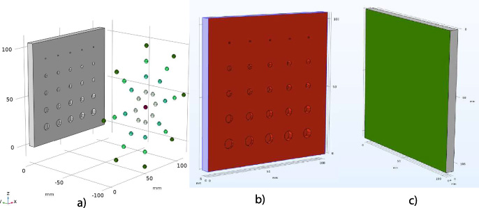
The geometry of the numerical model: (a) full setup — the sample and the heating device depicted as 33 point sources, (b) the rear side (RS) of the sample — heated one, (c) the front side (FS) of the sample — observed one.
One of the most important and basic tasks related to the issues of training neural networks is to create an appropriate database. In this article, the database will be built only using the numerical data, and its effectiveness will be checked on both: numerical and experimental data, where the latter were not fed to the network training. In order for the trained network to be effective, the numerical data should be strongly correlated with the experimental ones. It is also important to process and carefully select the data. In this chapter, first the experimental and numerical results will be compared. Then, the method of data processing by subtracting the trend and normalization will be presented. In the last step the process of the data selection for the NN training will be explained.
The comparison between the numerical and experimental data
The results were obtained as a sequence of 360 images having a size of 220 × 220 pixels, thus the whole database contains 48400 time-temperature characteristics. The Fig. 4 shows an example of the temperature distribution (captured at t = 60 s — the end of the heating period) on the surface of the test sample obtained experimentally (Fig. 4(a)) and numerically (Fig. 4(b)). A significant similarity of the obtained results can be observed, especially when it comes to the number of visible defects. The maximum temperature obtained for the numercial result for this frame is 314.36 K, which is 2.37 K higher than in the experiment.
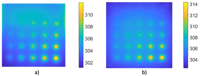
Exemplary thermogram (for t = 60 s) obtained experimentally (a) and numerically (b).
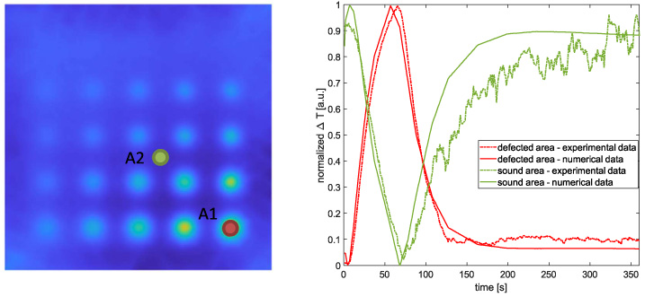
In order to assess the fit of the numerical model to the results of the experiment, the comparison of the time-temperature characteristics averaged from the selected areas (A1 - the area within the selected defect and A2 - the area without defects) is presentred in Fig. 5. As can be seen, the general characteristics of the curves are consistent for both of these areas, there are slight deviations in the values not exceeding 13% of the value range.
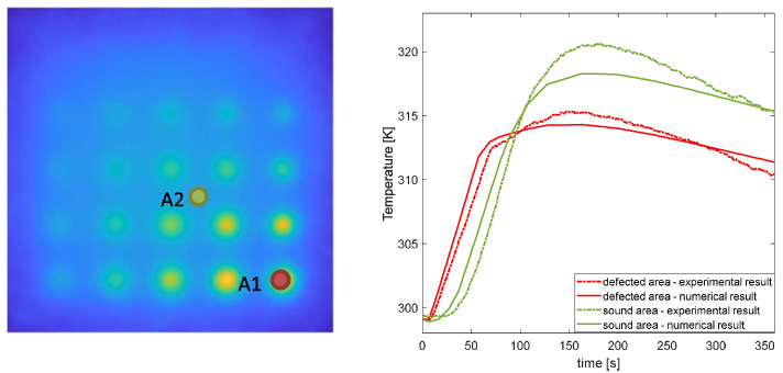
The comparison of the time-temperature characteristics for the experimental and numerical data. The characteristics were plotted as the mean values of the pixels from defected area A1 - localized within the defect with 7 mm diameter and 4.2 mm depth (red lines) and sound area A2 (green lines).
The compliance of time-temperature characteristics was also tested quantitatively. For each pixel, the correlation between the time-temperature characteristics obtained numerically and experimentally was calculated. As a result, the value of linear correlation coefficient was obtained for each pixel and these values were plotted as a correlation map (Fig. 6). As can be easily seen, the correlation coefficients range from 0.85 to 0.99.

The linear correlation coefficients map.
The halogen lamp used in the experiment as a heat source has a certain directional heating characteristic, resulting in uneven heating of the test sample (this effect was also roughly repeated in the numerical simulation). The results can therefore be significantly improved if the trend resulting from uneven lamp heating is removed from the obtained thermograms. In this paper, the removal of the trend by the surface fitting method for each thermogram in the sequence was used. The procedure is shown in Fig. 7. The least squares method was used to approximate the temperature distribution of the thermogram, assuming the approximating function in the form of a 6-th degree polynomial in two variables (Fig. 7(a)). The approximating surface thus obtained reflects the trend resulting from uneven heating with the lamp, but not the defects themselves, which are relatively small disturbances in the temperature distribution (see Fig. 7(b) with the surface and the thermogram overlapped). The area obtained in the procedure of the approximation is subtracted from the original thermogram. Finally, the trend leveling and improvement in the visibility of defects is obtained (see the comparison between the data before the trend removal — Fig. 7(c) and after it Fig. 7(d)). Another method of trend removal is based on estimation of background temperature distribution using a 2D filtering with median or Gaussian filter. In this case the size of moving window should be noticeable bigger than the size of smallest possible defects. Such method is utilized in case of X-ray evaluation [15]. The advantage of the method using approximation in relation to the filtering method is faster operation for the image sequence — the approximation coefficients calculated for the previous sequence are transferred to the calculations in the next sequence, which significantly reduces the computational complexity and computation time.
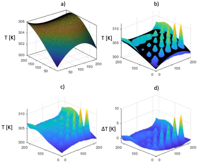
The procedure of the trend removal shown for exemplary thermogram from the sequence: (a) the approximated surface obtained with 6-th order polynomial in two variables, (b) the surface and the thermogram data overlapped, (c) the thermogram before the trend removal, (d) the same thermogram after trend removal.
The Fig. 8 shows a comparison of selected thermograms obtained experimentally and numerically (again for t = 60 s), which were subjected to the process of trend removal. It can be seen that the background of both thermograms is more homogeneous and that all but the smallest (diameter equal to 1.4 mm) defects are visible. The last stage was the normalization of the obtained results. The Fig. 9 shows a comparison of the time-temperature characteristics averaged for pixels from the defect area and the area without defect, obtained from the sequence after subtracting the trend. Just like in the previous case, the character of the numerical and experimental curves remains consistent. For the characteristics within the defect range, the difference between the numerical and experimental data does not exceed 10% of the value range.

Exemplary thermogram after the trend removal (for t = 60 s) obtained experimentally (a) and numerically (b).
The comparison of the time-temperature characteristics for the experimental and numerical data after the procedure of trend removal. Again the characteristics were plotted as the mean values of the pixels from defected area A1 - localized within the defect with 7 mm diameter and 4.2 mm depth (red lines) and sound area A2 (green lines).
As mentioned earlier, both numerical and experimental data were used at the last stage of work on the automatic defect recognition procedure. The results of both experiments were placed in two sets. First, a set of numerical data was used during the process of selecting the structure and configuration of the neural network. Before this work was carried out, three subgroups were distinguished in the data set: training, validation, and testing. Each of the subgroups contained a unique representation of all cases. To avoid the problem of favoring any cases, first, based on the knowledge about the actual defect location, 26 subgroups of signals were distinguished: a subgroup representing the area without a defect and 25 for subsequent defects. Then the representatives of individual subgroups were randomly divided between the training, validation and testing set, keeping all cases equal in each set. In the case of defects with the smallest diameters, the database was supplemented with additional ones created on the basis of real signals modified with the use of noises with random instantaneous values. Finally, the database was divided in the ratio of 0.7: 0.15: 0.15 into training, validation and testing sets, where the two classes: “defect” (containing data from 25 groups) and “non-defect” were defined.
In case of the experimental results, whole representation was used for the testing in the obtained NN performance verification stage.
Deep learning-based defect indication procedure
Considering that the defects occurring in the tested object have both a short-term and long-term effect on the time-temperature characteristics, a structure based on a unidirectional LSTM network was used to implement the final procedure of automatic defect recognition.
LSTM neural network structure
As an assumption, automatic detection of defects was carried out in relation to the prediction of the areas of occurrence and absence of defects in the tested object. Thus, it is the task of classification with the distinction of two classes. Therefore, five basic layers can be distinguished in the general structure of the used LSTM network. The network begins with an input layer, to which a vector (a time-series of 360 values) of the temperature distribution at a given point on the sample surface is fed. The next layer is LSTM one. During the work, a simple unidirectional LSTM structure was used. Compared to classic RNNs, the LSTM network architecture is modified by introducing a gating mechanism replacing the classic activation functions [10,14,16,17]. LSTM cells have three gates: input, forget, and output. As a result, they enable the modification of the cell state vector and memorizing many dependencies with different dynamics. Then, to predict class labels, the network ends with a sequence of three classifying layers: fully connected, softmax and classification output. The fully connected is a flattened one-dimensional array of the previous layer, where each neuron is connected to each neuron from the previous layer, and each connection has its own weight. The probability value of belonging of the input vector to a specific class is calculated in the softmax layer using the normalized exponential (softmax) function [18]:
During the selection of the final LSTM network configuration, preliminary experiments were carried out considering the 6 different size of the LSTM layer ranging from 30 to 1080. The calculations were also carried out for different network depths using one and two successive LSTM layers. Moreover, to minimize the risk of an overfitting problem, a dropout layer was used in the network structure. As a result of the dropout, individual neurons are randomly removed from the layers during the learning process. The probability of removing a given neuron in the next round of the learning process was changed from 20% to 90%. For each configuration, the calculations were performed five times, and then the result with the highest network accuracy value for the test set was selected. Considering the reduction of the computational time required for the whole optimization process, a stochastic gradient-based approximation method Adam was used during the training with an initial learning rate set to 10−3 to avoid overfitting [19]. The mini-batch size was set to 51 and maximum epochs number to 200. The final structure and configuration of the LSTM network obtained as a result of the performed preliminary experiments is presented in Fig. 10.
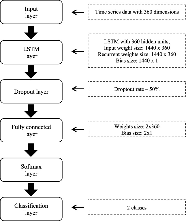
Final structure of the LSTM neural network.
For the verification of the trained LSTM network structure, the classification was run over the testing set. The confusion matrix of network is presented in Table 2. The rows correspond to the predicted classes and the columns to actual ones of the testing sets. The actual non-defect case was ascribed as negative class (N) while the defect occurrence was identified as the positive one (P). The percentage of properly classified defects is at good level equal to 96.5%. Additionally, several other coefficients allowing the assessment of the network performance under different aspects were calculated [20]. The true positive rate TPR (called sensitivity or recall):
Confusion matrix of the obtained final network.
Note: TP — true positive; FP — false positive; TN — true negative; FN — false negative.
To visualize the operation of the obtained LSTM network, the existence prediction of the classes over the whole surface of the tested object was performed for the numerical simulation data. The obtained distribution is presented in Fig. 11(a). It can be noted that practically the occurrence of all defects was properly indicated. The highest misclassification rate concerns the cases of the defects having the smallest diameter as not all were indicated. The comparison of the predicted state and the actual one over the objected surface can be seen in Fig. 11(b), where both states were marked with different colors. One can notice that although the defects occurrence was generally correctly assessed, the true area covered by defects is not so precisely pointed. This may be because the material located in the close vicinity of the defect is, in a way, a transition area between the defect-free and defect state. Such an area is not completely healthy, but there is no defect in it either. Nevertheless, the response of the infrared radiation characteristic for this region differs from both cases, which in turn results in over-marking of the predicted defect area.
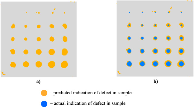
Results of the LSTM neural network validation stage achieved for numerical simulation data for whole sample: (a) visualization of the predicted (depicted with orange) indication of defects existence and position over the sample surface, (b) visualization of both predicted (orange) and actual (blue) indication of defect over the sample surface.
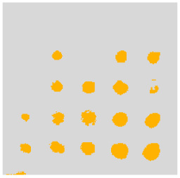
Visualization of the predicted (depicted with orange) indication of defects existence and position over the sample surface carried out for measurement results.
Final verification was carried out for the data obtained during the measurements. Similarly, as for the numerical simulation results, the obtained LSTM network was also applied to measured sequences of temperature distribution. The predicted indication of the defects distribution over the object surface can be seen in Fig. 12. One can notice that even though the measured characteristics have not been considered in the LSTM network training, mostly, the occurrence of the defects was predicted properly. Only the defects with the smallest diameter were not indicated at all. The other groups can be generally noticed with fairly good rate.
In the presented study the main goal was to develop a technique for thermographic evaluation of real (3D printed) samples using neural networks trained on numerical data (obtained using finite element method based computation). This approach is highly dependent on quality of numerical model and its compliance with the measuring experiment conditions. Thanks to proper modelling of halogen lamp based heat source and its directional radiation characteristics, similar temperature distributions were obtained using both simulations and measurements. This similarity was evaluated quantitatively using correlation coefficient. The calculated over entire surface correlation coefficients ranged from 0.85 to 0.99, what clearly indicates the high quality of numerical model and all the assumptions made during simulation process (including material physical properties). Moreover, in order to reduce the influence of the mentioned halogen lamp directional radiation characteristics, surface fitting procedure was proposed and verified. This procedure allowed to reduce the background temperature distribution and in consequence have enabled the creation of a more general database, that can be the basis for automating the process of assessing structures tested with the thermovision method. A LSTM neural network was selected for the task of automatic detection of defects. Its structure was optimized on the basis of a series of preliminary experiments. The proposed LSTM network shows good defect indication probability (both sensitivity and specificity are over 96%) while maintaining low level of false calls at the same time. Concluding, most of the defects were detected as well as their positions were predicted properly. The proposed method has been inefficient only in the case of the defects having the smallest diameter (𝜙 =1.4 mm) which were classified as non-defect in case of 2 most shallow ones (depth equal to 1.4 mm and 2.1 mm) for the numerical data and were not indicated at all in the experimental data. However, the detection of such defects should be considered as a hard case, which barely influences the local heat distribution in the sample characterized by the low value of thermal conductivity (such as the tested in this paper).
Footnotes
Acknowledgements
This research was funded by the National Science Center, Poland (Narodowe Centrum Nauki, NCN), within the research project “Evaluation of the internal structure and assessment of the structure health of complex materials using active infrared thermography with multiple excitation sources”, grant number 2020/04/X/ST7/01388. The APC was funded by the Research Fund of the Faculty of Electrical Engineering (West Pomeranian University of Technology, Szczecin, Poland).