Research on lane identification based on deep learning

Abstract

In order to meet the real-time and robustness requirement of driverless cars driving on highway, this paper proposed a lane line identification method based on the Deep Learning. This method first built a lane line image library and then input the pictures of the lane line image for denoising and normalized processing. Secondly, the Lenet – 5 network model was used for classification and recognition, with a recognition rate of 99.4%, and the lane line type was displayed through GUI interface. Finally, this method was compared with the support vector machine and BP neural network, and the results effectively verified that the method can satisfy the requirement of real-time and accuracy of lane line identification.

Keywords

Image processing lane line identification convolutional neural network deep learning

1. Introduction

With the continuous development of image processing technology, many research schools have applied this technology to environmental awareness and achieved good result in lane line identification, an important technology in unmanned driving. This technology not only requires lane line image with recognition rate, but also strictly demands for real-time and robustness.

The research of lane line recognition mainly adopts the following methods: the Support Vector Machine (SVM) [1] method mainly uses prior knowledge and artificial designed machine model [2], which can identify whether a model design could affect the final recognition results or not, but it could not ensure the recognition rate; The BP neural network [3] method has a good self-learning ability, but the design model requires the manually designed weight, threshold value and the number of iterations, which can easily lead to the fitting; for the detection method of hough transform, [4] in case of a road with seriously damaged or blurred lane lines, the recognition rate will be low and the robustness is not good enough to meet the visual technology.

In this paper, Deep Learning is applied to the classification and identification of lane lines, and the feature extraction and recognition of lane lines is made by constructing a seven-layer network model. Meanwhile, the image preprocessing of binarization and denoising is added in the experiment, and the collected images are made into training sets and test sets. By comparing different methods, it is effective to verify that this method has a good recognition effect.

2. The research methods

2.1 SVM (support vector machine)

Support vector machine (SVM) is a general machine learning method which is trainable and based on the principle of structural risk minimization. The principle of SVM method is the process of linearization and dimensionality. SVM is developed from the optimal classification hyperplane in the case of linear separability. As shown in the Fig. 1, hollow points and solid points represent two types of samples respectively. H is the h-dimensional classification hyperplane, HI and H2 are hyperplanes that are over various points and closest to the classification hyperplane for example and parallel to H. The optimal classification hyperplane theory requires the classification hyperplane to maximize the classification interval on the basis of correctly separating the two types.

Figure 1.

SVM schematic.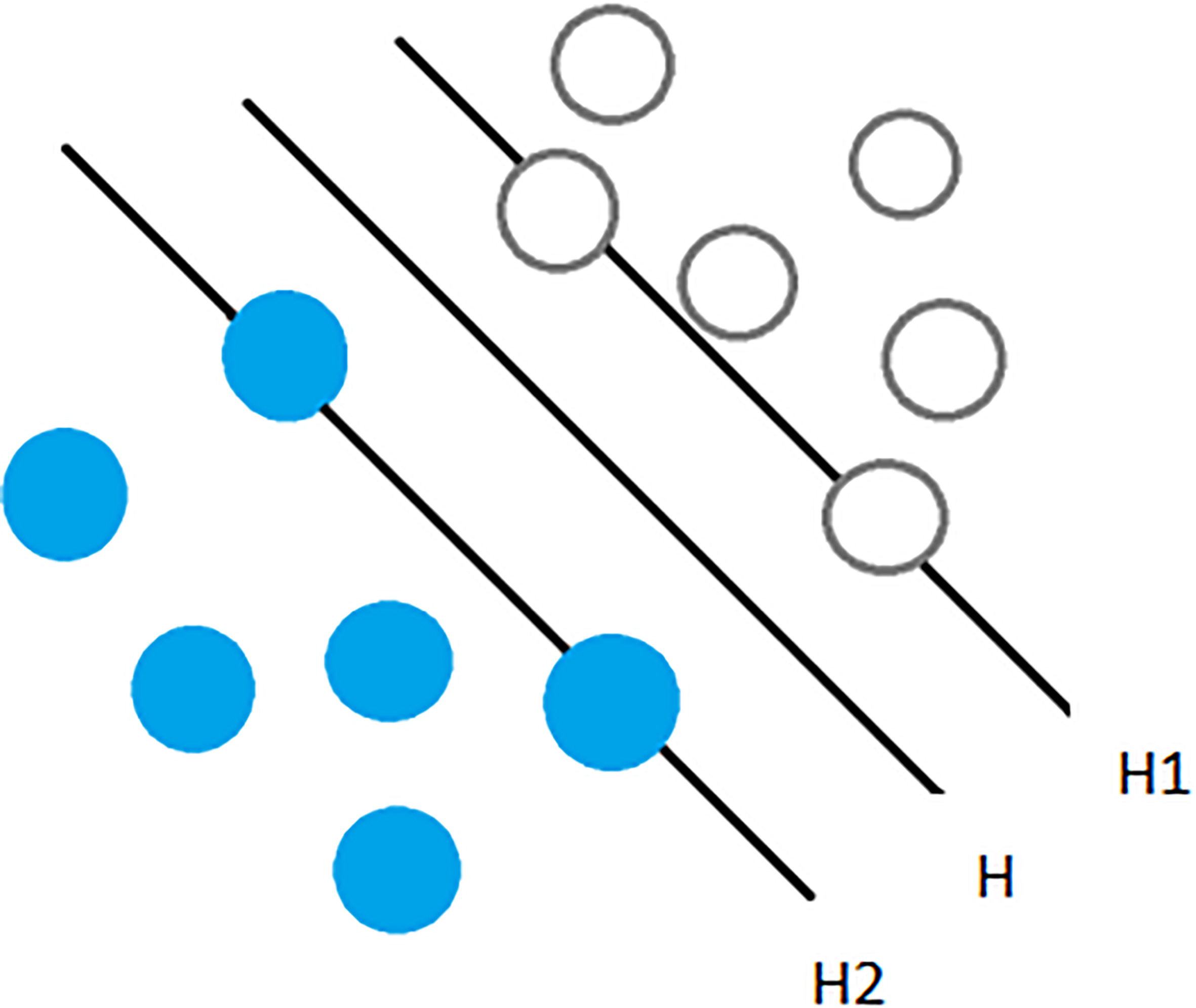

Obviously, the SVM has a better classification, but it’s harder to train for large-scale data training. Therefore, SVM is not adopted as the research method in this paper.

2.2 BP neural network

The basic principle of BP learning algorithm is gradient descent method. By adjusting the power values, the network is minimized. At the time of the signal propagation phase, the input is processed through the input layer, the sublayer is processed, the output is processed through the layer, and finally the output is processed. In the phase of error back propagation, the output signal value of the output layer is compared with the expected output signal value to obtain the error. If the error is large, the error signal will be sent back to the hidden layer until the input layer. In each layer of neurons, the error signal is used to modify the weight coefficient, and then the next iteration is conducted. The Fig. 2 shows a simple BP neural network model.

Figure 2.

BP neural network model.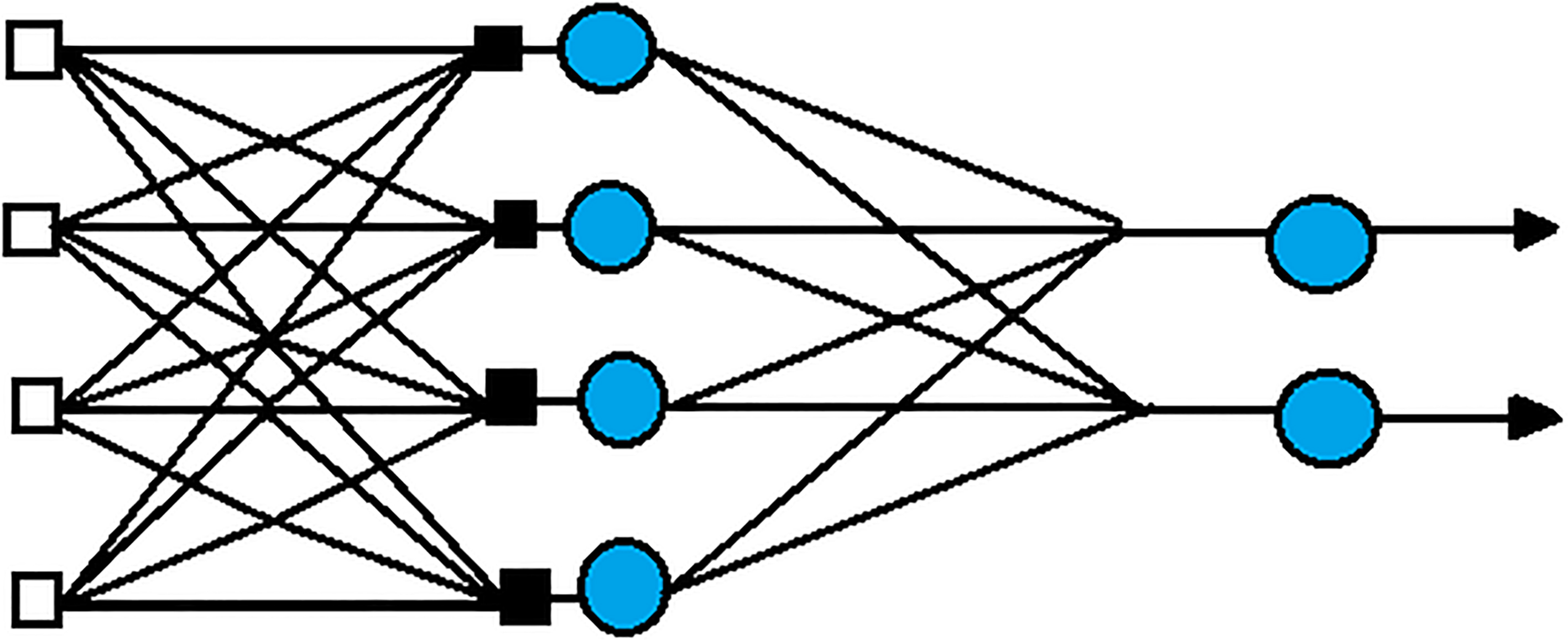

According to the above principle, BP neural network has a better fault tolerance. However, the complex processing results in a slow operation speed, so this paper does not use BP neural network as recognition method.

2.3 Deep learning

In 2006, the field of artificial intelligence, Hinton published an article about Deep Learning in science [5], which caused a new wave of Deep Learning in all walks of life. Deep learning [6] is designed to imitate the visual perception of human brain. By taking the convolution layer and the lower sampling layer, the image can be extracted and transformed layer by layer, so that the characteristics can be studied more effectively. At present, Deep Learning has been applied in many fields, such as handwriting recognition [7], license plate character recognition [8], traffic sign recognition [9], face recognition [10] and so on. In this paper, lane line identification is based on deep learning framework. The recognition under classification is different from general models, such as convolutional neural network (CNN) [11], which is the deep learning under a model framework. The network structure of the design is shown in Fig. 3.

Figure 3.

Convolutional neural network structure.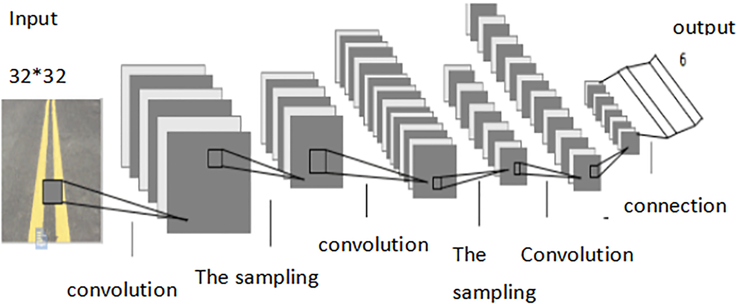

3. Results and discussion

Before the feature extraction of the image, it is necessary to preprocess the image, so the image input to the network is generally 32*32 pixels. Considering the number and parameters of the network structure layer, the image input into the network should be small as possible, so that the real time can be improved. The network structure is shown in Table 1.

Table 1
A seven-layer convolution neural network layers

No.	Type	C.kernels	Neurons	Characteristics
0	Input layer		32*32
1	Convolution layer	5*5	28*28	6
2	Sample layer	2*2	14*14	6
3	Convolution layer	5*5	10*10	16
4	Sample layer	2*2	5*5	16
5	Convolution layer		1024
6	Output layer		6

3.1 Image pre-processing

In the process of acquiring lane line images, there are many factors that may lead to interference, such as vehicle, shade, long-term wear of lane line and so on. In order to make the image characteristics better, so you need to do image preprocessing. The image preprocessing in this paper is to expand the sample size, mainly including image binarization, image denoising and others.

3.2 The characteristics of the convolutional neural network

The three characteristics of the convolution neural network are: local sensing field [12], descending sampling and weight sharing [13], which enables the network model invariable to translate, scale and deform in other forms. The local perception field is to reduce the number of training parameters, shorten the time and meet the real-time requirement. Weight sharing is designed to reduce the number of parameters per layer and network complexity. The convolutional neural network not only has the self-learning ability of traditional machine learning, but also has the advantages of automatic feature extraction [14].

3.3 The operation of the convolutional neural network

3.3.1 Forward propagation

In the forward propagation process of the convolutional neural network, the collected images are taken by the convolution layer. The characteristics of convolution layer is extracted and transferred to the pooling layer. Then the whole connection layer is processed, and the output layer is finally classified and recognized.

In the convolution process, the convolution layer is the two-dimensional convolution of the input image of the input layer or previous pooling layer and the non-linear excitation function, which can be expressed in Eq. (1):

$\displaystyle G_{k}^{l}=f\left(\sum\limits_{i=1}^{M_{l-1}}{G_{i}^{l-1}}\ast Q_% {ik}^{l}+b_{k}^{l}\right)$ (1)

In the formula: $G_{k}^{l}$ is the output of the k convolution feature subgraph in the first layer; $M_{l-1}$ is the total output of the previous layer; $Q_{{ik}}^{l}$ is the weight of the $k^{\rm th}$ convolution in the $l^{\rm th}$ layer; $b_{k}^{l}$ is the threshold value of $k^{th}$ convolution in the first layer; symbol “*” denotes to two dimensional convolution operation; $f()$ is a nonlinear excitation function, which can be expressed by Eq. (2):

$\displaystyle f(x)=\frac{1}{1+{e}^{-x}}$ (2)

In the formula: $x$ is the input of the function.

The pooling layer is the sampling of the convolution layer output. The characteristics of the output after the pooling will be reduced by k, and the Eq. (3) can be expressed as:

$\displaystyle G_{k}^{l+1}=\text{down}\ (G_{k}^{l})$ (3)

In the formula: $G_{k}^{l+1}$ represents the output of the $k^{th}$ sampling in the $l+1$ layer; $G_{k}^{l}$ is the characteristic of $l$ layer output; down () is the sampling of the characteristics in the pooling.

3.3.2 Back propagation

The reverse propagation of the convolution neural network is the process of weight and threshold correction in the model, and the propagation error is minimized. Therefore, the activation function chosen is expressed as follows.

$\displaystyle f(x)=\frac{A}{1+e^{-\frac{w}{B}}}$ (4)

Using gradient descent method, the weight and threshold of the hidden layer and the output layer are adjusted. The adjustment is as follows:

$\displaystyle{w}_{{ik}}=w_{ik}-\eta_{1}\cdot\delta_{i{k}}\cdot x_{i}$ (5) $\displaystyle{b}_{k}=b_{k}-\eta_{2}\cdot\delta_{i{k}}$ (6)

Changes to the weight and threshold of the input and hidden layers are as follows:

$\displaystyle{w}_{{ki}}=w_{ki}-\eta_{1}\cdot\delta_{ki}\cdot x_{k}$ (7) $\displaystyle{b}_{i}=b_{i}-\eta_{2}\cdot\delta_{ki}$ (8)

3.3.3 The sampling

In the convolution neural network model, the convolution layer is trained by extracting the characteristics of the input layer. When the image size is large, the network training time will be very long. In order to maintain the real time, the convolutional neural network will connect a lower sampling layer after the convolution layer. The basic principle of the bottom sampling is that the image has a relatively static property, and the statistical property of the image in one region is similar to that of the adjacent region [15]. In addition to reducing the occurrence of the fitting, it can also reduce the operation time.

4. Experiment and analysis

4.1 Sample selection and pretreatment

The six types of lane lines that are common in China are selected as subjects: double yellow solid line, single yellow solid line, single white solid line, single white dotted line, single yellow dashed line and cross road crossing line. Training samples and test samples of lane line are selected from the shot images. Then, the samples receive denoising, binarization processing and other image pre-processings, to obtain more samples and make their network to adapt to severe environment. As shown in Fig. 4, after image preprocessing, such as binarization, noise processing and acquisition of the original image. In the process of filming, both the used camera and lane lines have relative velocity, and the shades of the trees and other factors may bring interference, so the obatined images may be not so clear, with much reflection. However, the designed network can adapt to various bad environment.

Figure 4.

Part of lane line samples.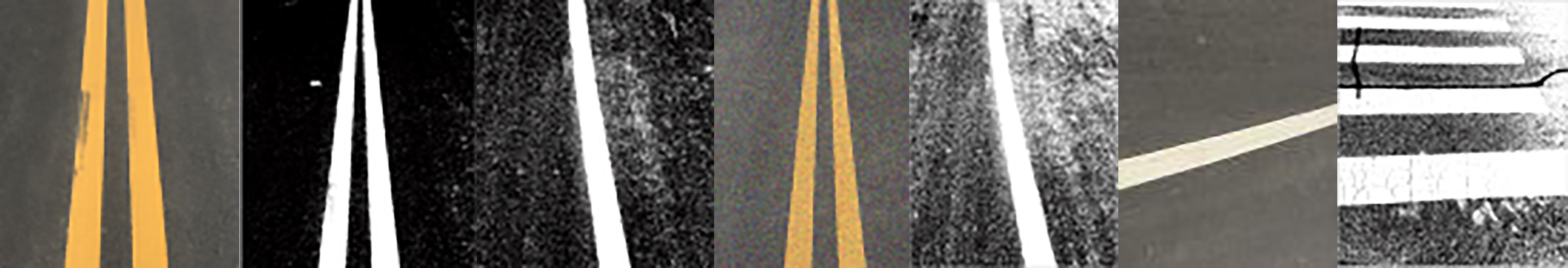

The collected lane line images were made into training set and test set. Before inputting the pictures in the model, they have to be pre-processed first, such as binarization and denoising. After that, the images were normalized to 32*32 pixels and input in the CNN network. In total, there are 548 training samples and 230 test samples.

4.1.1 Image binarization

Image binarization is to set the image pixel to 0 to 255, and at the same time reduce image data quantity. This highlights the image edge, thus improving the image detection and the real-time and accuracy of image recognition.

Figure 5.

Contrast of image binarization effect.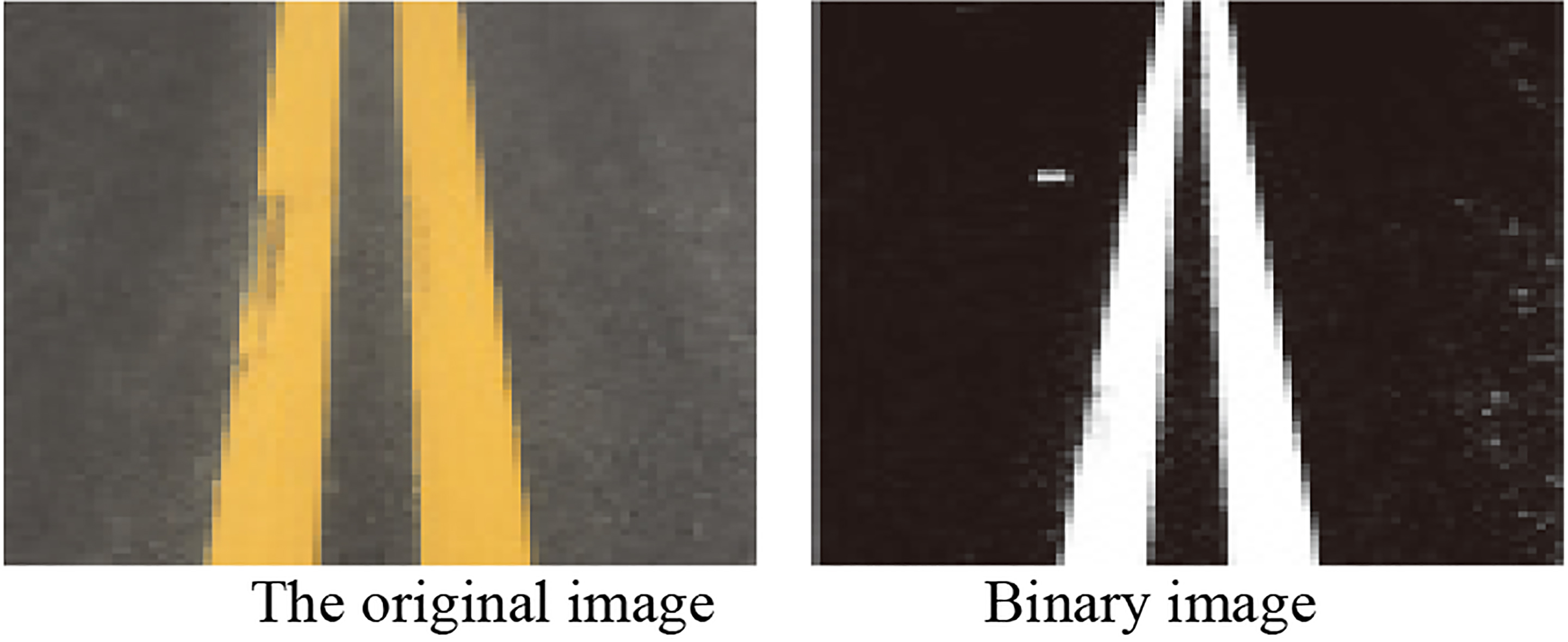

4.1.2 Image denoising

After image preprocessing, there will be some noise, which may degrade image quality and affect image detection and image recognition. Denoising can not only provide better image but also better support for recognition system.

Figure 6.

Contrast of image denoising effect.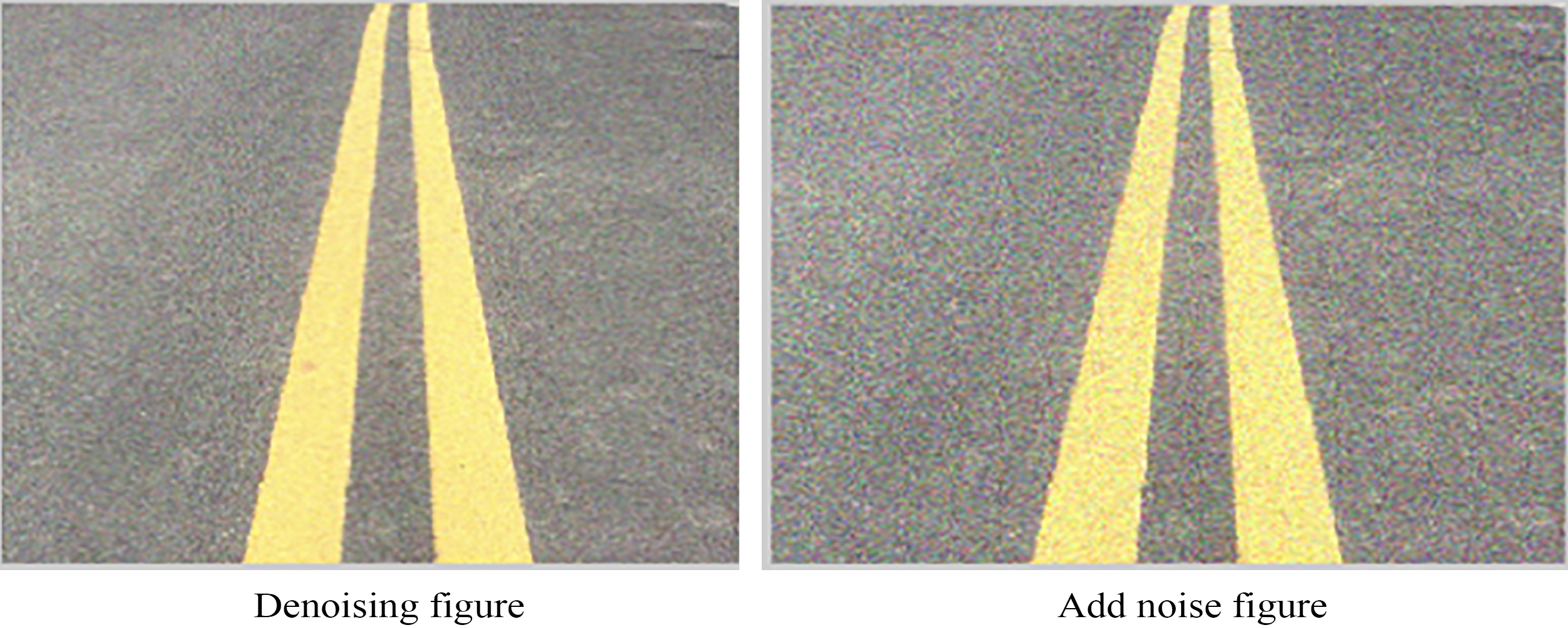

4.1.3 Image normalization

Image normalization is a uniform format image obtained after image processing. This is to ensure that the processed images do not affect the experimental results.

4.2 The main interface display

The following figures show the interface of lane identification, which is based on the GUI interface compiled by the tensorflow. It is mainly a recognition of the test sample and identified by inputting images under different conditions. This is shown in Figs 7 and 8.

Figure 7.

Double yellow lane line identification.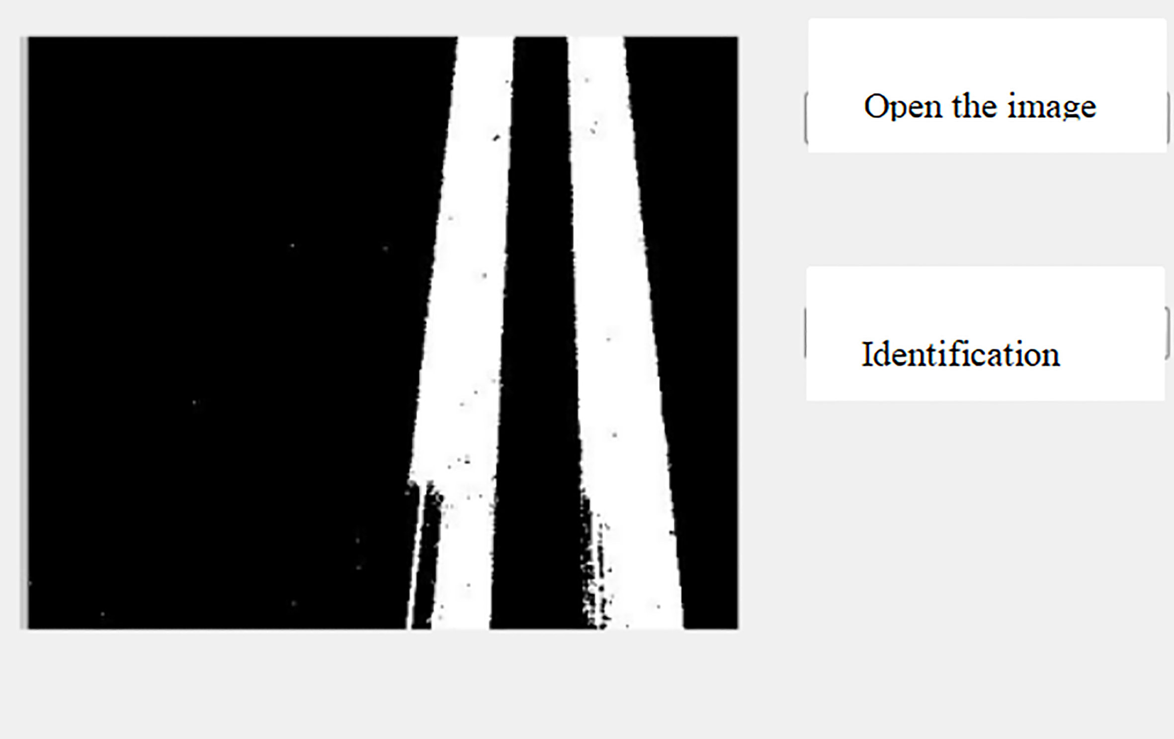

Figure 8.

Crosswalk identification.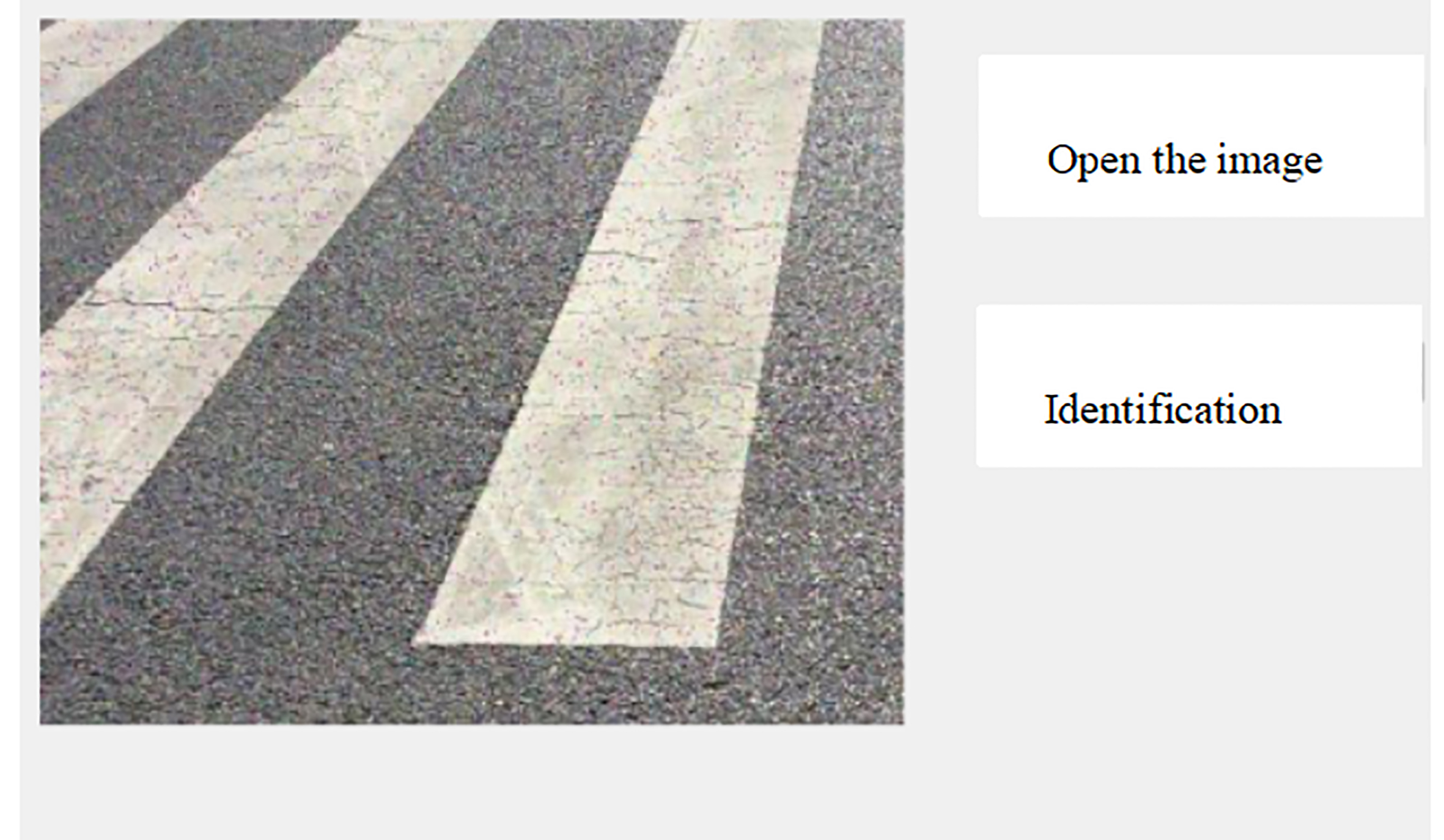

4.3 Experimental comparison and analysis

Some existing lane line location methods are used to classify the training samples and test samples, and convolution neural network is utilized to test the test samples. Totally, 230 test samples are classified into 6 types.

After the analysis of the experimental results, a total of 6 types of input networks were put into the lane line. After network classification, the detection accuracy reached to 99.4% and the experimental results were very significant.

In order to validate the advantage of the network, BP neural network and SVM were compared. The classification method used in this paper has a high accuracy, can adapt to the scenes under weak light, high salt and pepper noise and gaussian noise as well as with fuzzy lane line.

Compared with the traditional support vector machine and BP neural network, the recognition rate of the convolution neural network method is significantly higher. The comparison results are shown in Table 2.

Table 2
Comparison of recognition rates

Classification method	Parameter	Recognition rate
Convolutional neural network	Input: 32*32 Output: 6 The network structure: 7	99.4%
Support vector machine	Kernel function: Radial basis function Penalty factor: 78.15 Kernel parameter: 9.80	86.12%
BP neural network	Vector: 0.01 Hidden node number: 600 The network structure: 3	90.46%

The learning rate is 0.001, the number of iterations is 50, and the error rate and the recognition rate are shown in Fig. 9. The error rate and the recognition rate at the step 40 to 50 are basically stable, and the final recognition rate is 99.4%.

Figure 9.

Recognition rate and error rate.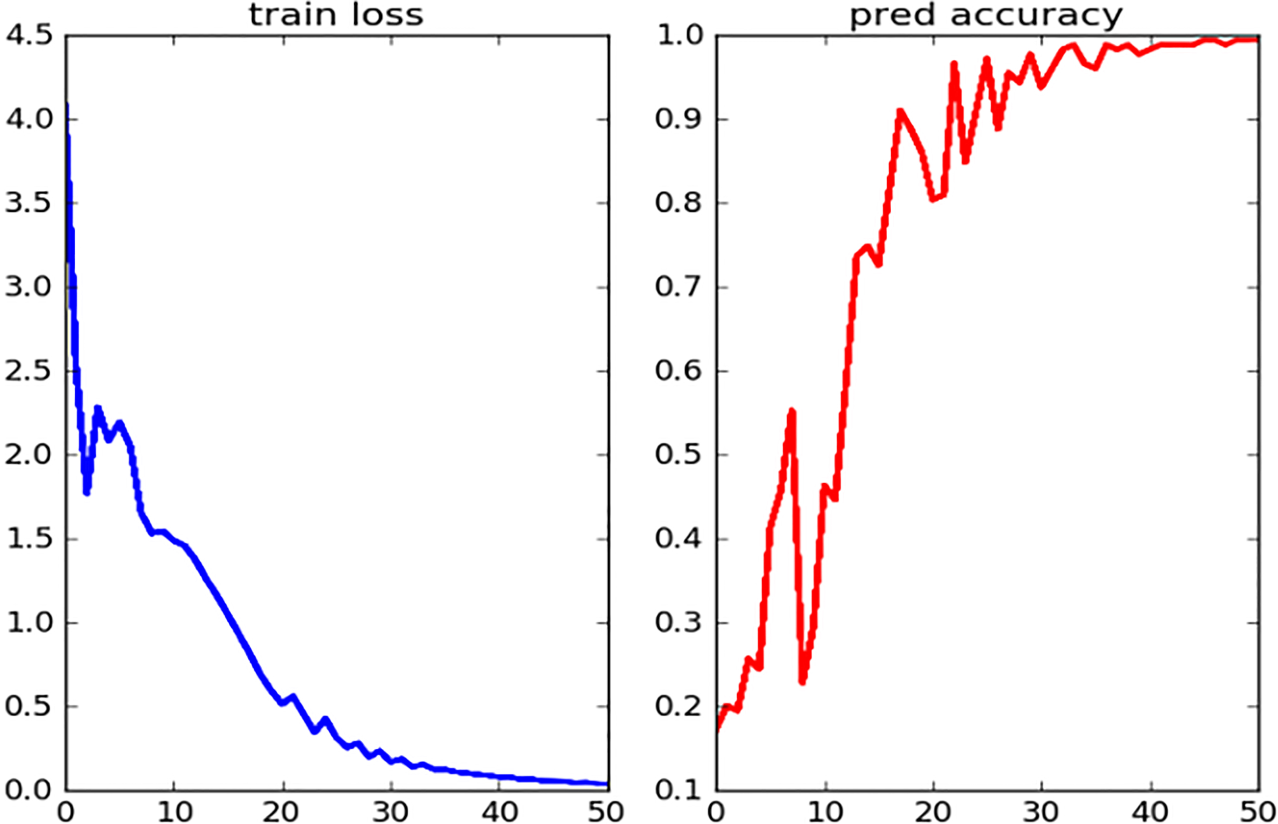

5. Conclusion

A seven-layer convolutional neural network was used to classify the lane lines using images provided by training samples. The experimental results show that, for the scenes with low light intensity, high pretzel noise and high gaussian noise, fuzzy lane line scene can be well adapted. The network structure has a recognition rate of 99.4% and can be tested in different scenarios. Compared with traditional methods, deep learning has higher recognition rate and so is of great significance in research. However, this method could not well recognize lane lines shot at night, which will be the main research content in the next step.

Footnotes

Acknowledgments

The authors acknowledge the National Key R&D Program of China (2018YFC0808203), Supported by Foundation of Shaanxi Key Laboratory of Integrated and Intelligent Navigation (SKLIIN-20180101).

References

Kazemi

F.M.

Samadi

Poorreza

H.R.

et al., Vechicle recognition using Curvelet transform and SVM[C]//Proc of the 4th International Conference on Information Technology: IEEE Press, 2007, 516–521.

Huang

and Zhang

, Identification of traffic signs using deep convolutional neural network, Modern Electronic Technology (13) (2015), 101–106.

Niu

and Li

, Application of neural network and bayesian filter in the prediction of change of channel, Science and Technology and Engineering (14) (2016), 212–216.

Niu

Zhang

and Li

, The lane line recognition algorithm based on machine vision, Journal of Tianjin Vocational and Technical Normal University (3) (2015), 16–19.

Hinton

G.E.

and Salakhutdinov

, Reducing the dimensionality of data with neural networks, Science 313(504) (2006).

Jia

and Chen

, Deep learning yesterday, today and tomorrow, Computer Research and Development (9) (2013), 1799–1804.

Song

and Yu

, Study on handwritten digital classification based on deep learning, Journal of Chongqing Technology and Business University (Natural Science Edition) (8) (2015), 49–53.

Zhao

Yang

and Ma

, Study on license plate character recognition of lenet-5 based on convolution neural network, Journal of System Simulation (3) (2010), 638–641.

Lin

and Zhang

, Identification of traffic signs using deep convolutional neural networks, Modern Electronic Technology (13) (2015), 101–106.

10.

Yang

Liu

and Fang

, Research on face recognition method based on deep learning, Journal of Tianjin University of Science and Technology (6) (2016), 1–10.

11.

Krizhevsky

Sutskever

and Hinton

G.E.

, ImageNet Classification with Deep Convolutional Neural Networks, Advances in Neural Information Processing System 25(2) (2012), 1097–1105.

12.

Lecunn

, Generalization and network design strategies, In connection and network design strategies in connection in perspective: University of Toronto, 1989.

13.

Silver

Huang

Maddison

C.J.

et al., Mastering the game of Go with deep neural networks and tree search, Nature 529(7597) (2016), 484–489.

14.

Chen

, Study on deep learning algorithm and application of convolutional neural network, Hangzhou: zhejiang university of commerce and technology, 2014.

15.

, Application of convolutional neural network in image classification, Sichuan: university of electronic science and technology, 2015.