Automatic classification and recognition of geomagnetic interference events based on machine learning

Abstract

Geomagnetic interference events seriously affect normal analysis of geomagnetic observation data, and the existing manual identification methods are inefficient. Based on the data of China Geomagnetic Observation Network from 2010 to 2020, a sample data set including high voltage direct current transmission (HVDC) interference events, other interference events and normal events is constructed. By introducing machine learning algorithms, three geomagnetic interference event recognition models GIEC-SVM, GIEC-MLP, GIEC-CNN are designed based on support vector machines (SVM), multi-layer perceptron (MLP) and convolutional neural networks (CNN) respectively. The classification accuracy for each model on the test set reached 76.77%, 84.96% and 94.00%. Two optimal GIEC-MLP and GIEC-CNN are selected and applied to the identification of geomagnetic interference events at stations not participated in training and testing from January, 2019 to June, 2021. The accuracy are 72.11% and 78.24% respectively, while the efficiency is 150 times that of manual identification. It shows that the geomagnetic interference event recognition algorithm based on machine learning algorithm has high recognition accuracy and strong generalization ability, especially the CNN algorithm.

Keywords

Geomagnetic interference automatic recognition machine learning HVDC CNN

1. Introduction

Geomagnetic observation data is important basic data for the study of seismic-geomagnetic relationship, earthquake prediction and geomagnetic storm prediction [1, 2]. Zhang et al. [3] used the membership function method to extract earthquake precursor anomalies in geomagnetic observation data; Yuan et al. [4] used the first-order difference method to extract earthquake precursor signals from geomagnetic data; Xu et al. [5] studied the relationship between the strength and weakness of the geomagnetic spectrum before and after the Jiuzhaigou Ms7.0 earthquake; Feng et al. [6] analyzed the relationship between earthquakes in the north-south belt of the Chinese mainland and the distribution of induced currents due to magnetic variation; Isa et al. [7] calculated the daily ratio of the geomagnetic vertical component of geomagnetic observation stations, and analyzed the relationship between the daily ratio anomaly characteristics and strong earthquakes in Xinjiang. At present, a digital geomagnetic observation network covering the whole China mainland has been established as shown in Fig. 1. There are 173 geomagnetic stations and 328 geomagnetic relative observation instruments. The seconds-sampled geomagnetic observation data includes: horizontal intensity H, vertical component Z, magnetic declination D, magnetic inclination I, total intensity F, etc.

Figure 1.

Distribution of China Geomagnetic Observation Network.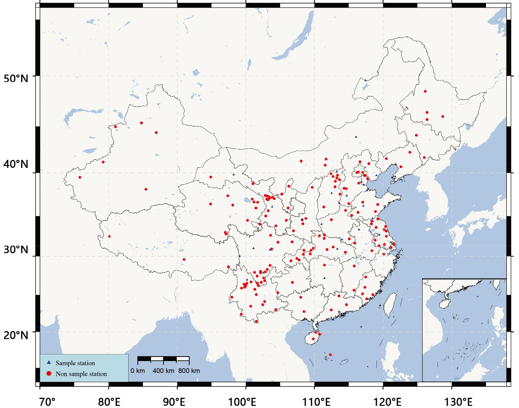

With the rapid development of economy, geomagnetic observation is seriously interfered by subways, light rails, and power grids [8, 9, 10]. According to statistics, there are 287 geomagnetic relative observation instruments in the country that are affected by the interference of high-voltage direct current transmission (HVDC), accounting for 87.5% of the total number of instruments. These interference events have severely affected the quality of geomagnetic observation data and restricted the study of seismic-geomagnetic relationships. To ensure the quality of the observation data, the front-line staff of stations currently mark and preprocess various interference events based on their professional knowledge and work experience, and then the staff of the National Geomagnetic Network Center will manually review them. With the implementation of the China Earthquake Science Experimental Field Project and the National Earthquake Monitoring Station Network Reconstruction and Expansion Project, the scale of geomagnetic stations and observation instruments will expand rapidly and exponentially. The existing manual identification of interference events will be difficult to meet the demand for massive data processing.

Researchers have developed a variety of geomagnetic interference event classification (GIEC) algorithms. Typical algorithms include first-order difference [11], polarization method [12], membership function [3], wavelet transform [13], empirical mode decomposition [14] and other methods. These mathematical or statistical methods are used to compare and analyze the magnitude of the data changes in different periods or compare with the observation data of reference stations in the same period. Then the observation data whose amplitude changes exceed the threshold are screened out [15]. Researchers determine the interference category based on work experience and expert knowledge, and the labor cost is very high. To replace the manual recognition, researchers have tried to develop automatic recognition technology for geomagnetic interference events. Chen et al. [11] compared the geomagnetic observation data of a certain station with the observation data of a reference station, and designed a high-accuracy HVDC interference automatic recognition system using the first-order difference method. This algorithm needs to set different thresholds for different station instruments, so the degree of automation is low. Yang et al. [16] used the same idea and used the first-order difference and reference component slope backcalculation method to propose a method that can automatically identify spike and step type geomagnetic interference events, but the disadvantage is that a suitable reference station must be selected for each station. It is assumed that no interference event occurs at the reference station at the same time. Its application conditions are relatively harsh. In addition, the universality of this method is still poor, which is only effective for regular HVDC interference events, and cannot identify other types of interference events such as traffic and infrastructure impacts.

In recent years, machine learning (ML) algorithms have achieved great success in the fields of image recognition [17], speech recognition [18], and natural language processing [19], etc. Researchers try to apply ML methods such as support vector machines (SVM), random forests, decision trees, and neural networks to geomagnetic data reconstruction [20, 21, 22], magnetic anomaly detection [23, 24, 25], earthquake precursor anomaly detection [26], geomagnetic storm prediction [27], seismic-geomagnetic relationship research [28] and other fields of geomagnetic data processing. Deep Neural Networks (DNN) represented by Convolutional Neural Networks (CNN) and Recurrent Neural Networks (RNN) have stronger automatic feature extraction performance, which has shown great potential in this field [24].

Geomagnetic observation data and manual preprocessed data from stations across the country from January 2010 to December 2020 are used to construct a sample set of geomagnetic interference events. SVM, multi-layer perceptron (MLP) and CNN are introduced to build GIEC-SVM, GIEC-MLP and GIEC-CNN geomagnetic interference event recognition models, respectively. The accuracy on the test set reached 76.77%, 84.96% and 94.00% respectively. To further test the effectiveness of the method, the GIEC-MLP and GIEC-CNN models with high accuracy were selected and applied to the identification of geomagnetic interference events at stations from January 2019 to June 2021. With a total of 7113 samples, the experimental results show that the two models completed the recognition work within 30 seconds, with accuracy of 72.11% and 78.24%, respectively, indicating that the geomagnetic interference event recognition algorithm based on the ML algorithm has good recognition accuracy and strong generalization ability. Compared with traditional manual identification, the processing time is greatly shortened, which effectively reduces the burden of preprocessing and review.

2. Data and preprocessing

In order to discuss the technology of geomagnetic interference events recognition using ML algorithms, the raw observation data recorded by the National Geomagnetic Station Network and the preprocessed data after manual interference removal from 2010 to 2020 are used to construct a sample data set. The data set recorded more than 2 million preprocessed records and more than 30 types of interference. Among them, the number of interference categories affected by HVDC is the largest, as many as 410,000, which is much higher than the number of other interference events such as vehicle impact, infrastructure project impact, and ground resistivity observation impact. Given the extremely uneven distribution of various interference categories, which may affect the accuracy and generalization ability of machine learning recognition, this article treats the impact of HVDC as a separate interference category, while the other interference events are unified into another category. The observation data of non-interference events is classified as normal.

The construction process of the sample set is as follows:

(1)
Select the D, H, Z converted data (that is, the minute-sampled data produced by Gaussian filtering of the raw seconds-sampled data) and manual preprocessed data of the GM series of geomagnetic observation instruments in Mengcheng, Changli, Shexian, Hongshan, Xilinhot, Jiayuguan, Lushi, Lanzhou, Xinyang, Yingcheng, Batang, Chongzhou, Qianling, Lijiang, Taiyuan, Dalian, Datong, Gaoyou, Jinghai, Tancheng, Shaoyang, Dao Fu, Xichang, Manzhouli, Tai’an, Wudi, Xuzhuangzi Station (the blue stations in Fig. 1) from 2010 to 2020 as the data source.
(2)
The converted sub-data of D, H, Z components produced by each observation instrument is taken as a sample every half an hour, and 48 samples are generated every day. If the sample lacks a certain component data or a component has more than 5 consecutive missing values, delete the sample data, otherwise replaced it with the previous value.
(3)
Calculate the difference between the converted minute-data of the sample and the manual preprocessed data. If the maximum variation of any one of the components is greater than the threshold 0.5, it is considered that the sample has an interference event, otherwise it is regarded as normal observation data and marked it as $-$ 1.
(4)
In the previous step, if the sample is considered to have an interference event, query the manual preprocessed log records of the instrument during the corresponding period. If it is a HVDC interference, mark it as 1, otherwise mark it as 0.
(5)
Standardize the sample observation data.

After the above steps, a total of 50,000 HVDC interference event samples were generated. Since the number of normal samples and other interference event samples is much larger than the number of HVDC interference event samples, considering the balance of data samples, 50,000 samples are randomly selected from normal samples and other interference event samples so that the sample size ratio of the three categories is 1:1:1.

Table 1
List of sample quantity

[height=1cm,width=2cm]QuantityCategory Normal Other HVDC

Training set 34000 34000 34000

Validation set 8500 8500 8500

Test set 7500 7500 7500

Total 50000 50000 50000

3. Method

[height=1cm,width=2cm]QuantityCategory	Normal	Other	HVDC
Training set	34000	34000	34000
Validation set	8500	8500	8500
Test set	7500	7500	7500
Total	50000	50000	50000

The identification of geomagnetic interference is essentially a classification problem. First, based on the classic SVM machine learning method, the geomagnetic interference event recognition model GIEC-SVM is constructed. Second, considering the great success of deep learning networks achieved in recent years, we construct a geomagnetic interference event recognition model GIEC-MLP based on MLP and a geomagnetic interference event recognition model GIEC-CNN based on CNN.

3.1 GIEC-SVM method

The SVM algorithm was proposed by Corinna Cortes et al. [29]. It is used to find a hyperplane with the largest separation in the feature space, so that the distance between various sample points and the hyperplane is the farthest. It has been widely used in classification recognition, sequence prediction and other fields. Dixit et al. [30] used the SVM algorithm to build a diagnostic framework for COVID-19 patients, and the recognition accuracy was as high as 99.34%; Ma et al. [31] used SVM to predict and monitor the flue gas temperature in the airtight process of roadway fires; Xu et al. [32] constructed a prediction model of dynamic measuring pressure of storage silo wall base on SVM and optimized SVM hyperparameters by cross validation and grid search method. Zheng et al. [33] used SVM to represent the human control strategy by the parametric model without knowledge of the actual robot mathematical model.

SVM is a two-classification model. However the samples of geomagnetic interference events in this article are divided into three categories: normal, HVDC interference and other interference, which is a multi-classification task. To enable SVM to achieve multi-classification tasks, multiple SVM classifiers need to be constructed and trained. There are two main strategies: One-Versus-One (OVO) and One-Versus-Rest (OVR).

In the SVM-OVO method, it is necessary to design an SVM classifier for any two types of samples, and use the corresponding sample sets for training. Therefore, if there are K categories, K*(K-1)/2 SVM classifiers need to be constructed. When classifying a new sample, the sample needs to be input into all SVM classifiers, and the category with the most votes is the final category of the new sample. In the SVM-OVR method, samples of a certain category are classified into one category, and samples of other categories are classified into another one. At this time, K categories need to construct K SVM classifiers, and train them separately according to the classification of corresponding samples. When classifying a new sample, it is necessary to input the sample into the above K SVM classifiers to obtain a classification result respectively, and select the largest one of the K values as the classification result. The advantage of the SVM-OVO classification method is that the generalization ability is strong as the samples are balanced, but when there are many categories, more classifiers need to be built, and the cost of model training is quite high. The advantage of the SVM-OVR algorithm is that the number of SVM classifiers to be built is small, and the classification training speed is relatively fast. The disadvantage is that the generalization ability of the model is often poor due to the uneven number of samples.

In the classification task of geomagnetic interference events in this paper, there are 3 categories, so the value of K is 3, and both algorithms need 3 SVM classifiers. This article uses the sklearn library to create the above two SVM classifiers, and chooses the Gaussian kernel as the kernel function to implement the nonlinear classification task.

3.2 GIEC-MLP method

MLP is also known as fully connected neural network, in which each layer is composed of multiple neurons and usually divided into input layer, hidden layer and output layer. Each output of the lower layer is used as the input of the higher layer, as shown in Fig. 2. The network can automatically learn effective feature representations from a large amount of input data. In recent years, it has performed well in image classification [34, 35] and other fields, which is easy to parallelize and has high generalization ability.

Figure 2.

GIEC-MLP network structure.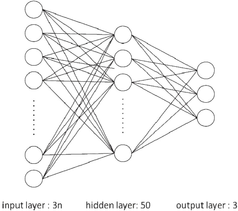

The GIEC-MLP constructed in this paper based on the multilayer perceptron is shown in Fig. 2, which includes an input layer, a hidden layer and an output layer. Since there is only one hidden layer, the model can also be regarded as a shallow neural network structure. Because this article takes the D, H, and Z data of an instrument as a sample every 30 minutes, the number of input layers of this network model is the number of all observations in a sample, that is, 3*n, where 3 means three components of D, H, Z, n is 30 observed value. The number of neurons in the middle hidden layer is set to 50, and the number of neurons in the output layer is the number of classification tasks, which is 3. To enhance the nonlinear expression ability of the model, GIEC-MLP selects the Sigmoid activation function.

3.3 GIEC-CNN method

Deep learning networks, especially CNN, are widely used in anomaly detection [36], time series classification [37], seismic event classification [38], earthquake location [39] and other fields, and achieved good application results. CNN introduces hidden layers such as convolutional layer and pooling layer based on MLP. It greatly reduces the number of neural network parameters through local connection and sharing-parameters, reduces storage consumption, and improves computing efficiency. Through multiple convolution kernels of different sizes and multi-layer convolution stacking, various local morphological feature information of the input data can be captured, which has strong robustness and fault tolerance, and is easier to train and optimize [40].

Figure 3.

GIEC-CNN network structure.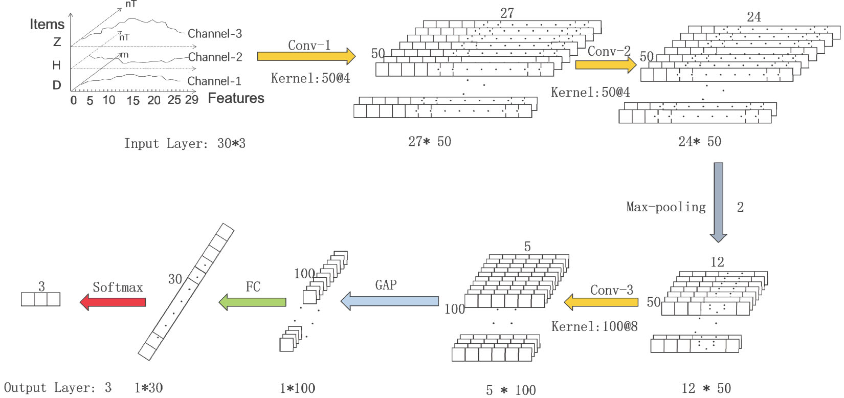

The GIEC-CNN network structure is shown in Fig. 3, which consists of an input layer, a convolutional layer, a pooling layer, a fully connected layer, and an output layer. Among them, it contains 3 convolutional layers to extract different features of the input data; 1 maximum pooling layer and 1 global average pooling layer. As an effective dimensionality reduction method, the pooling layer can remove the redundant information compress data features, enhance non-linear features, expand the perceptual field of view, simplify network complexity, reduce network parameters, calculations and memory consumption, and achieve translation invariance, rotation invariance and scale invariance.

(1)

Input layer: Since each data sample contains 30 values of the D, H, and Z components of the geomagnetic observation instrument, the D, H, and Z components are input to the convolutional layer as three channels, so the input layer is a 30 *3 matrix.

(2)

Convolutional layer Conv-1: defines 50 convolution kernels of length 4, and outputs a 27*50 neuron matrix after convolution operation.

(3)

Convolutional layer Conv-2: Like the convolutional layer Conv-1, 50 convolution kernels of length 4 are still used, and the output matrix size is 24*50.

(4)

Maximum pooling layer Max-pooling: After the convolutional layer, the maximum pooling layer is introduced, the pooling size is set to 2, and the output matrix size of this layer is 12*50.

(5)

Convolutional layer Conv-3: This layer defines 100 convolution kernels with a length of 8 to extract higher-level data features, and the output matrix size is 5*100.

(6)

Global average pooling layer GAP: Global average pooling layer can greatly reduce network parameters and avoid over-fitting. The output matrix size of this layer is 1*100.

(7)

Fully connected layer FC: The number of output neurons is set to 30.

(8)

Softmax layer: This layer uses Softmax as the activation function, and the number of neurons is the number of output categories 3.

Since the features of geomagnetic interference event data are nonlinear, the introduction of activation functions can enhance the nonlinear feature extraction ability of the neural network and strengthen the learning ability of the neural network. The ReLU activation function effectively solves the problem of the disappearance of the gradient. Besides, the calculation speed is fast, and the convergence speed is also faster than the Sigmod and tanh activation functions. Therefore, in the above-mentioned layers, except for the 8th layer, all other layers select ReLU as the activation function.

When training a deep network model, an optimizer based on gradient descent is usually used to minimize the loss function. This article chooses the Adam (Adaptive Moment Estimation) optimizer. Adam uses the exponentially weighted average of gradients and the exponentially weighted average of gradient squares to dynamically adjust the learning rate of each parameter. The initial value of the learning rate is set to “0.01”. In order to prevent overfitting, the weight decay rate is set to 1e-08.

4. Experiment and results

The test environment of this article is a desktop computer configured with an Intel Core i9-10900K CPU (3.70 GHz, 10 cores), 64 GB memory, Windows 10 Enterprise Edition operating system and 512 GB hard drive. GPU is 1 Nvidia Tesla V100 (16 GB). This article uses the sklearn library to build the GIEC-SVM model and Keras open source framework to build GIEC-MLP and GIEC-CNN models.

In order to compare and analyze the classification effects of different models, this article uses accuracy, recall and precision indicators for comparative analysis. Table 2 shows the confusion matrix between the predicted and true values of the geomagnetic interference category classification model in this paper. Among them, TP (True Positive) means that the prediction is correct, that is, the true value of the sample is the same as the predicted value, which is expressed in bold font; FP (False Positive) indicates a prediction error, that is, the true value of the sample and the predicted value are not the same.

Table 2
Confusion matrix

[height=1cm,width=2.9cm]Actual value Predictive value	$-$ 1	0	1
$-$ 1	$\textit{TP}_{-1}$	$\textit{FP}_{1}$	$\textit{FP}_{2}$
0	$\textit{FP}_{3}$	$\textit{TP}_{0}$	$\textit{FP}_{4}$
1	$\textit{FP}_{5}$	$\textit{FP}_{6}$	$\textit{TP}_{1}$

The accuracy is the ratio of the number of samples that the model predicts correctly to the total number of samples, namely:

$\displaystyle A=\frac{\textit{TP}_{-1}+\textit{TP}_{0}+\textit{TP}_{1}}{% \textit{TP}_{-1}+\textit{FP}_{1}+\textit{FP}_{2}+\textit{FP}_{3}+\textit{TP}_{% 0}+\textit{FP}_{4}+\textit{FP}_{5}+\textit{FP}_{6}+\textit{TP}_{1}}\times 100\%$ (1)

Precision refers to that the proportion of samples whose predictions are positive. To calculate the precision of the model, the precision of each category is calculated at first. The precision of the normal category $P_{-1}$ is defined as shown in Eq. (2).

$\displaystyle P_{-1}=\frac{\textit{TP}_{-1}}{\textit{TP}_{-1}+\textit{FP}_{3}+% \textit{FP}_{5}}\times 100\%$ (2)

Similarly, the precision of other interference category is:

$\displaystyle P_{0}=\frac{\textit{TP}_{0}}{\textit{TP}_{0}+\textit{FP}_{1}+% \textit{FP}_{6}}\times 100\%$ (3)

The precision of HVDC interference category is:

$\displaystyle P_{1}=\frac{\textit{TP}_{1}}{\textit{TP}_{1}+\textit{FP}_{2}+% \textit{FP}_{4}}\times 100\%$ (4)

Since the sample sizes of the three categories in the sample in this article are the same, the precision of the model is defined as the average of the precision of the three categories, namely:

$P=\frac{P_{-1}+P_{0}+P_{1}}{3}$ (5)

Recall refers to the proportion of samples predicted to be positive among all samples whose true value is positive. Taking the normal category as an example, the recall can be defined:

$\displaystyle R_{-1}=\frac{\textit{TP}_{-1}}{\textit{TP}_{-1}+\textit{FP}_{1}+% \textit{FP}_{2}}\times 100\%$ (6)

In the same way, the recall of the other interference category and HVDC interference category are defined as shown in Eqs (7) and (8), respectively.

$\displaystyle R_{0}=\frac{\textit{TP}_{0}}{\textit{TP}_{0}+\textit{FP}_{3}+% \textit{FP}_{4}}\times 100\%$ (7) $\displaystyle R_{1}=\frac{\textit{TP}_{1}}{\textit{TP}_{1}+\textit{FP}_{5}+% \textit{FP}_{6}}\times 100\%$ (8)

In the same way, the recall of the model is defined as the average of the recall of 3 categories, namely:

$\displaystyle R=\frac{R_{-1}+R_{0}+R_{1}}{3}$ (9)

4.1 GIEC-SVM experimental results

Combine the training set and validation set samples, and then reorganize the samples for training and testing according to the OVO and OVR strategies. The kernel function selects the Gaussian kernel function. Experimental results show that the highest accuracy of SVM-OVO and SVM-OVR on the training set are 79.67% and 79.63% respectively; the accuracy on the test set are 76.50% and 76.77% respectively, the precision are 78.89% and 79.14% respectively, and the recall are 77.60% and 77.94% respectively. It can be seen that the accuracy of the model on the test set and the training set is equivalent, the accuracy of the model is low, and the classification ability is poor; the classification performance of the two strategies of OVO and OVR is not much different.

4.2 GIEC-MLP experimental results

In the GIEC-MLP network model, the initial value of the learning rate is set to 0.01. In order to obtain the optimal model, an Early Stopping strategy is adopted, that is, the loss (val_loss) indicator of the monitoring model on the verification set. If the indicator does not improve after 30 consecutive iterations, the model is considered to be optimal and stop training automatically. The changes in accuracy and loss during the training of the GIEC-MLP model are shown in Fig. 4. In the end, the accuracy of the model on the training set and validation set are 88.55% and 84.48% respectively. On the test set, the accuracy is 84.96%, the precision is 84.85%, and the recall is 84.76%. It can be seen from Fig. 4 that as the number of iterations increases, the accuracy of the model on the training set continues to increase, and the loss continues to decrease, while the accuracy of the model on the validation set does not increase significantly. The loss tends to stabilize, indicating that the model has over-fitting phenomenon. Compared with the GIEC-SVM model, the classification accuracy of the GIEC-MLP model is further improved, indicating that the model has a stronger classification performance.

4.3 GIEC-CNN experimental results

In the training process of the GIEC-CNN model, the same early stopping strategy as the GIEC-MLP model is still adopted. The accuracy and loss changes during the training process are shown in Fig. 5. The accuracy of the model on the training set and validation set are 95.00% and 94.54% respectively. On the test set, the accuracy is 94.00%, the precision is 94.27%, and the recall is 94.24%. It can be seen from Fig. 5 that the model fits well on the training set and the test set, and there is no obvious over-fitting phenomenon, and the accuracy of the model is significantly higher than that of the GIEC-SVM and GIEC-MLP models. GIEC-CNN has strong classification performance.

5. Results analysis and application test

Based on the above models, the accuracy, recall, precision and loss of the geomagnetic interference event recognition model in the training set, verification set and test set are analyzed as shown in Table 3.

Table 3
Model accuracy, precision, recall and loss

Algorithms	Training set		Validation set		Test set
	Accuracy	Loss	Accuracy	Loss	Accuracy	Recall	Precision	Loss
GIEC-SVM (OVO)	79.67%	/	/	/	76.50%	77.60%	78.89%	/
GIEC-SVM (OVR)	79.63%	/	/	/	76.77%	77.94%	79.14%	/
GIEC-MLP	88.55%	0.36	84.48%	0.42	84.96%	84.76%	84.85%	0.45
GIEC-CNN	95.00%	0.16	94.54%	0.19	94.00%	94.24%	94.27%	0.21

Figure 4.

MLP training curve.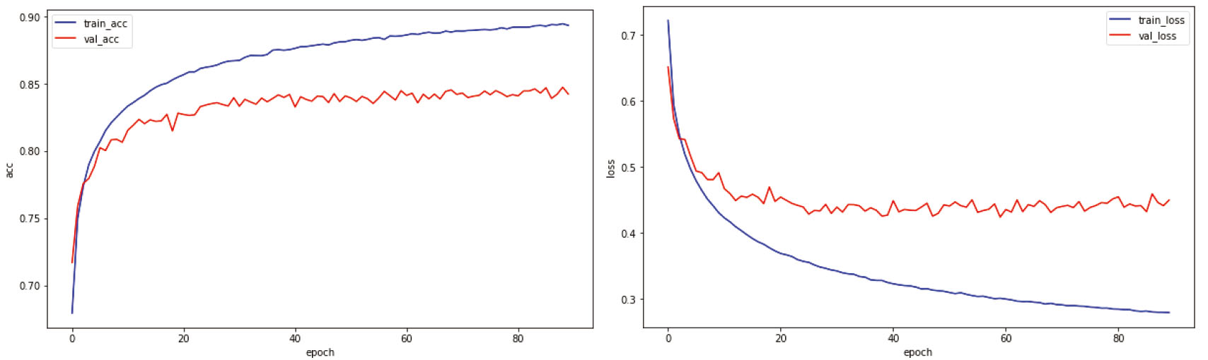

Figure 5.

CNN training process curve.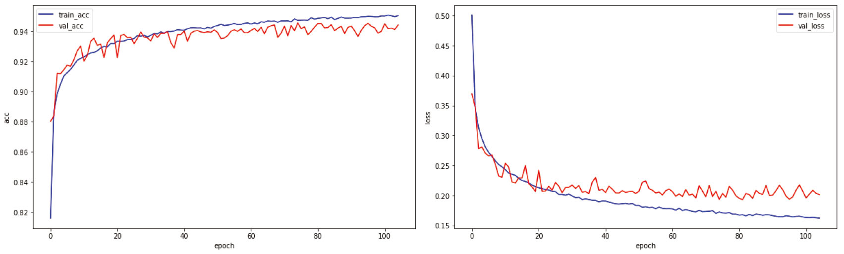

Since the SVM model combines both the training set and the validation set samples during training, we redivides the samples according to the algorithm needs. So the accuracy of the GIEC-SVM (OVO) and GIEC-SVM (OVR) models on the training set is actually the result of training on the training set and validation set. As can be seen from Table 3, the accuracy of GIEC-CNN model is the highest in both the training set and the verification set, which are 95.00% and 94.54% respectively, and the loss is the lowest, which are 0.16 and 0.19 respectively. In the test set, GIEC-CNN model had the highest accuracy, precision and recall (94.00%, 94.27% and 94.24%, respectively), followed by GIEC-MLP model, and GIEC-SVM model had the lowest. The results show that the neural network has a clear advantage over the traditional SVM model in automatic feature extraction of geomagnetic interference events. Especially with the increase of network depth, the feature extraction ability of the model is enhanced. The GIEC-CNN model is ahead of the other two models in all indicators. In addition, the accuracy, precision and recall of GIEC-CNN model on the test set all reached more than 94%, indicating that the model has good classification ability and certain practical value.

In order to further test the actual classification effect of the above geomagnetic interference event identification model, the observation data of stations that did not participate in training and testing from January 2019 to June 2021 were collected manually, and 7113 sample data were produced. The number of samples of normal category, HVDC interference event category and other event category was 2371 each. GIEC-SVM, GIEC-MLP and GIEC-CNN models are used for further testing.

The experimental results are shown in Table 4. GIEC-SVM still performed poorly. GIEC-CNN model is significantly superior to GIEC-MLP model in accuracy, precision and recall. However, the accuracy of GIEC-MLP and GIEC-CNN models only reached 72.11% and 78.24% in the new sample set respectively, lower than that of 84.96% and 94.00% on the test set before. To further analyze the reasons, the recognition results of each category of the two models are shown in Table 5. The number of correctly recognized categories is represented in bold. GIEC-MLP and GIEC-CNN correctly recognized 55.84% and 69.92% of the normal samples respectively. GIEC-CNN correctly recognized 82.62% of the other interference samples and 82.16% of the HVDC samples. GIEC-MLP correctly recognized 83.05% of the HVDC samples.

Table 4

Test results of GIEC-SVM,GIEC-MLP and GIEC-CNN models

Methods	Precision	Recall	Accuracy
GIEC-SVM (OVO)	65.23%	65.13%	65.13%
GIEC-SVM (OVR)	65.48%	65.40%	65.40%
GIEC-MLP	73.27%	72.11%	72.11%
GIEC-CNN	78.67%	78.24%	78.24%

Table 5

Confusion matrix of new data set

Real valuePredictive value	Normal		Other		HVDC
	GIEC-MLP	GIEC-CNN	GIEC-MLP	GIEC-CNN	GIEC-MLP	GIEC-CNN
Normal	1324	1658	271	309	776	404
Other	190	61	1836	1959	345	351
HVDC	311	318	91	105	1969	1948

In addition, the identification of all samples by GIEC-MLP and GIEC-CNN models on the experimental desktop computer in this paper was completed within 30 seconds. If the current method of manual visual inspection is followed, that is, each component of an instrument is manually reviewed, evaluated, re-processed and re-evaluated every day, it will take at least 30 seconds to check the daily data of one instrument. There are 7113 data samples in this experiment, and the cumulative time span is about 148 days for the observation data of one instrument. Using the above criteria, it would take at least 74 minutes to manually check. The efficiency of automatic identification is about 150 times that of manual identification, which greatly saves labor cost.

6. Conclusions and discussion

In this paper, machine learning algorithms are introduced and three machine learning-based methods for automatic identification of geomagnetic interference events are proposed. The experimental results show that the GIEC-MLP and GIEC-CNN models have much higher accuracy, recall and precision than the GIEC-SVM algorithm on the test set, with accuracy of 84.96% and 94.00%, respectively. It indicates that neural networks, especially deep learning networks, have strong feature extraction and nonlinear representation capabilities. The GIEC-MLP and GIEC- CNN models achieved 72.11% and 78.24% accuracy in application testing experiments in less than 30 seconds, which indicates that the models have certain generalization ability and greatly improve the efficiency relative to existing manual recognition.

As can be seen from Tables 4 and 5, the accuracy of GIEC-MLP and GIEC-CNN models are lower in the new data application experiments than testing set. There are 776 and 404 samples of normal category are identified as HVDC interference events, accounting for 32.73% and 17.04% of the 2731 samples, respectively; for the HVDC interference event category, both 2 models have more than 310 samples are identified as normal category. The main reasons for the analysis are as follows: (1) because of the complex morphological characteristics of geomagnetic interference events, the amplitude and morphology of the same interference event at different stations and at different times are different, which makes the automatic identification of geomagnetic interference events very difficult; (2) the samples are cut per 30 minutes, which may split the interference events, resulting in small feature differences between different sample categories and large feature difference between samples of the same category, which is difficult to distinguish; (3) this paper divides normal and interference samples by a threshold of 0.5, which may have the problem of misclassification and lead to inaccurate data features learned by the model. Therefore, to solve the above problems, the next step is to study reasonable sample division methods and sample category accurate labeling methods to improve the sample quality, and also try to optimize the CNN structure to improve the model recognition accuracy and generalization ability.

Footnotes

Acknowledgments

This research was supported by national key R&D plan (2018YFC1503806), the earthquake science and Technology Spark research project of China Earthquake Administration (XH20024).

The geomagnetic observation data is provided by National Geomagnetic Network Center, Institute of Geophysics, China Earthquake Administration.

References

. Physics of electromagnetic phenomena of the earth. Anhui: Press of University of Science and Technology of China, 2009.

Zhao

Liu

Mao

. Dependence of Great Geomagnetic Storm (ΔSYM-H⩽ – 200 nT) on Associated. Solar Wind Parameters Solar Physics. 2021; 296(4): 1-14. doi: 10.1007/s11207-021-01816-2.

Zhang

Qiao

. Precursory anomalies of geomagnetic field dynamic subordinate function method. Progress in Geophysics. 2005; 1: 142-6.

Yuan

Feng

Jiang

Pan

Qian

Yao

. Application of first-order difference method in the extraction of seismic geomagnetism precursor signal. Journal of Seismological Research. 2020; 43(4): 738-44+68.

Chen

Wang

. High frequency enhancement phenomenon of geomagnetism before the Jiuzhaigou Ms70. earthquake. Progress in Geophysics. 2021; 36(2): 525-30.

Feng

Jiang

Feng

Dai

Huang

, et al. A preliminary study on relationship between Induced current of geomagnetic diurnal variation with short-term reproducibility concentration distribution and earthquakes. Earthquake Research in China. 2020; 36(3): 502-16.

Aisa

Feng

Chen

Xin

Mao

, et al. Geomagnetic day by day ratio and its relationship with strong earthquakes in Xinjiang and its adjacent areas. Chinese Journal of Space Science. 2021; 41(4): 617-25.

Xiong

Liu

Liang

, et al. The application of large data mining techniques in earthquake precursory network observation data tracking analysis. Seismological and Geomagnetic Observation and Research. 2016; 37(3): 1-6.

Bao

Jiang

Fan

Zhang

. Study on the impact of high voltage direct current (HVDC) transmission interference on geotechnical stations in Jiangsu province. Earthquake Research in China. 2020; 36(3): 607-19.

10.

Fan

. A New compensation method for the magnetic interference of vehicle. Applied Mechanics and Materials. 2013; 373: 811-4.

11.

Chen

Jiang

Zhang

Chen

Yang

Liu

. The design of HVDC discrimination and processing system for geomagnetic network. Seismological and Geomagnetic Observation and Research. 2014; 35(Z2): 270-4.

12.

Zhang

Zhao

Jia

Liu

Teng

. Applying of polarization method to extract short term seismic anomaly from geomagnetic second data. Progress in Geophysics. 2020; 35(2): 488-94.

13.

Dou

Wang

Zheng

. Possible seismo-magnetic effect of the Wenchuan earthquake: Characteristics of ’difference in daily amplitude’ derived from the wavelet transform for the Z-components in geomagnetic observatories. Recent Developments in World Seismology. 2018; 4: 95-7.

14.

Zhang

Wang

Zhao

. Picking up geomagnetic pulsation using empirical mode decomposition. Seismological and Geomagnetic Observation and Research. 2014; 35(1): 114-20.

15.

Wang

Zhang

Jiang

Zhang

. Anomaly analysis of geomagnetic loading and unloading response ratio at Shexian geomagnetic station. Seismological and Geomagnetic Observation and Research. 2020; 41(4): 70-7.

16.

Yang

Wang

. Research on typical interference identification and processing methods of geomagnetic observation data. Plateau Earthquake Research. 2020; 32(3): 30-6+68.

17.

Özyurt

. Efficient deep feature selection for remote sensing image recognition with fused deep learning architectures. The Journal of Supercomputing. 2020; 76(11): 8413-31.

18.

Nassif

Shahin

Attili

Azzeh

Shaalan

. Speech recognition using deep neural networks: A systematic review. IEEE Access. 2019; 7: 19143-65.

19.

Maulud

Zeebaree

SRM

Jacksi

Sadeeq

MAM

Sharif

. State of art for semantic analysis of natural language processing. Qubahan Academic Journal. 2021; 1(2): 21-8.

20.

Liu

Bin

Shi

, et al. A nonlinear regression application via machine learning techniques for geomagnetic data reconstruction processing. IEEE Transactions on Geoscience and Remote Sensing. 2018; 57(1): 128-40.

21.

Chinchunair

DRT

. Neural network approach for reconstruction of geomagnetic data via machine learning. Solid State Technology. 2020; 63(6): 5806-14.

22.

Komala

Raju

, editors. A survey on a nonlinear regression application to machine learning techniques for geomagnetic data reconstruction processing. E3S Web of Conferences. 2020; EDP Sciences.

23.

Fan

Kang

Wang

HGH

Zhang

Liu

. Adaptive magnetic anomaly detection method using support vector machine. IEEE Geoscience and Remote Sensing Letters. 2020; 19: 1-5.

24.

Huang

Liu

Fang

. DeepMAD: Deep Learning for Magnetic Anomaly Detection and Denoising. IEEE Access. 2020; 8: 121257-66.

25.

Zheng

Fan

Yin

. A method of using geomagnetic anomaly to recognize objects based on HOG and 2D-AVMD. AIP Advances. 2019; 9(7): 075015.

26.

Cai

Shu

Teng

, Anomaly detection of earthquake precursor data using long short-term memory networks. Applied Geophysics. 2019; 16(3): 257-66.

27.

Tasistro-Hart

Grayver

Kuvshinov

. Probabilistic geomagnetic storm forecasting via deep learning. Journal of Geophysical Research: Space Physics. 2021; 126(1): e2020JA028228.

28.

Katori

Okubo

. Neural network based geomagnetic estimation for multi-site observation system. IEICE Communications Express. 2018; 7(10): 352-7.

29.

Cortes

Vapnik

. Support-vector networks. Machine Learning. 1995; 20(3): 273-97.

30.

Dixit

Mani

Bansal

. CoV2-Detect-Net: Design of COVID-19 prediction model based on hybrid DE-PSO with SVM using chest X-ray images. Information Sciences. 2021; 571: 676-692.

31.

Zhang

Guo

Wei

Zou

Wei

. GA-SVM model for prediction flue gas temperature of roadway fire under sealing process. Journal of China University of Mining & Technology. 2021; 50(4): 641-8.

32.

Liu

Yuan

. Dynamic lateral pressure prediction model of grain storage warehouse wall based on support vector machine. Journal of Agricultural Mechanization Research. 2022; 44(5): 9-16.

33.

Zheng

Sun

. Research on Motion Control for a Mobile Robot Using Learning Control Method. Applied Mathematics and Nonlinear Sciences. 2021; 6(1): 227-34.

34.

Zhang

Pan

Gardiner

Sargent

Hare

et al. A hybrid MLP-CNN classifier for very fine resolution remotely sensed image classification. ISPRS Journal of Photogrammetry and Remote Sensing. 2018; 140: 133-44.

35.

Sait

, Shivakumar

Kumar

Prajapati

Chakrapani

. A deep-learning based multimodal system for COVID-19 diagnosis using breathing sounds and chest X-ray images. Applied Soft Computing Journal. 2021; 109: 107522.

36.

Yin

Zhang

Wang

Xiong

. Anomaly detection based on convolutional recurrent autoencoder for Iot time series. IEEE Transactions on Systems, Man, and Cybernetics: Systems. 2020; 52(1): 112-22.

37.

Qian

Xiao

Zheng

Zhou

Zhuang

, et al. Dynamic multi-scale convolutional neural network for time series classification. IEEE Access. 2020; 8: 109732-46.

38.

Kim

Ahn

Lee

. Attention-based convolutional neural network for earthquake event classification. IEEE Geoscience and Remote Sensing Letters. 2020; 18(12): 2057-61.

39.

Perol

Gharbi

Denolle

. Convolutional neural network for earthquake detection and location. Science Advances. 2018; 4(2): e1700578.

40.

Zhou

Jin

Dong

. Review of convolutional neural network. Chinese Journal of Computers. 2017; 40(6): 1229-51.

Automatic classification and recognition of geomagnetic interference events based on machine learning

Abstract

Keywords

1. Introduction

3.1 GIEC-SVM method

3.2 GIEC-MLP method

Table 2 Confusion matrix

4.2 GIEC-MLP experimental results

4.3 GIEC-CNN experimental results

5. Results analysis and application test

Table 3 Model accuracy, precision, recall and loss

Footnotes

Acknowledgments

References

Table 2
Confusion matrix

Table 3
Model accuracy, precision, recall and loss