A convolutional-LSTM model for nitrogen oxide emission forecasting in FCC unit

Abstract

As the environment issue is put on the agenda, air pollution also concerns a lot. Nitrogen oxide (NOx) an is important factor which affects air pollution and is also the main gas emissions of the smoke and waste gas of FCC unit in petrochemical industry. It is important to accurately predict the NOx emission in advance for petrochemical industry to avoid air pollution incidents. In this paper, convolutional neural network (CNN) and long short-term memory (LSTM) are combined to predict the NOx emission in Fluid Catalytic Cracking unit (FCC unit). Convolutional-LSTM (CLSTM) is able to extract the spatial and temporal features which are essential information in the prediction of the NOx emission. The features in the factors of production which would affect the NOx emission are extracted by CNN which prepares time series data for LSTM. The LSTM layer is connected after CNN to model the irregular trends in time series. CNN, Multi-layer perception (MLP), rand forest (RF), support vector machine (SVM) and LSTM are implemented as baseline models. The results from the proposed CLSTM model showed better performance than all the baseline models. The mean absolute error and root mean square error for CLSTM were calculated with the values of 16.8267 and 23.7089 which are the lowest among all the models. The Pearson correlation coefficient and R2 for the proposed CLSTM model are calculated with the value of 0.9263, 0.8237 which are the highest among all the models. Furthermore, the residual graphs indicate the well matched performance between the observations and the predictions. The study provides a model reference for forecasting the NOx concentration emitted by FCC unit in petrochemical industry.

Keywords

Nitrogen oxides machine learning LSTM CNN

1 Introduction

Nitrogen oxide (NOx) is an important part of air pollution which mainly refers to nitric oxide (NO) and nitrogen dioxide (NO2) in the air. Reacting with oxygen, NO is easy to convert to NO2 due to the instability which is toxic to the human body. Furthermore, photochemical reactions would result in more toxic photochemical smog [1]. Besides, the main components of acid rain, nitric acid (HNO3) is also formed by the interaction of NO¬2 with water molecules which would acidify the soil and water resources. For Fluid Catalytic Cracking unit (FCC unit), NOx is one of major emissions released in the flue gas. To control the NOx emission and reduce the probability of air pollution, it is important for petrochemical industry to predict the NOx emission and perform corresponding measures in advance.

NOx emission forecasting is a prediction problem with multivariate time series [2]. Previous methods on forecasting time series mainly include: (1) the prediction analysis methods based on traditional statistics (e.g., autoregressive integrated moving average (ARIMA) [3]), and (2) the machine learning methods. However, it is very difficult to predict NOx emission of FCC unit using traditional statistical prediction methods because of the nonstationary of NOx emission data which contains irregular trends components and complex nonlinear relationship. Therefore, more and more researchers tend to use the machine learning methods.

Artificial neural network (ANN) is a kind of machine learning methods that imitates the mechanism of biological neuron. In 1962, multi-layer perception (MLP) model was proposed [4] which is a neural network with a fully-connected architecture with good performance. However, with the increase of complexity and amount of data, the MLP can hardly model the relationship between inputs and outputs.

Recent studies have shown that deep learning enhance the expressive ability and has broad prospects. In the field of image processing, convolutional neural network (CNN) [5] is superior to the existing methods. Long short-term memory (LSTM) [6, 7] have achieved excellent success in speech recognition and natural language processing (NLP). CNN can extract features of the input data and update the weights of the feature maps without the consideration of temporal information. LSTM stores and updates the long sequential information in hidden memory to capture the dynamics through time. However, in NOx emission prediction problem, the data is time series with various features, which cannot be fully utilized by conventional CNN and LSTM alone.

In this paper, a new architecture of deep neural networks based on the CNN and LSTM was proposed (refer to CLSTM hereafter) to predict NOx emission in FCC unit. This architecture combines the intrinsic advantages of CNN and LSTM which could be used by the petrochemical industries to predict NOx emission and adjust production plans. Some baseline methods (MLP, random forest (RF), support vector machine (SVM) and LSTM) were implemented and compared with CLSTM by mean absolute error (MAE), root mean square error (RMSE), Pearson correlation coefficient (PCCS) and coefficient of determination (R2). The major contribution of this paper is the proposal of a novel architecture which can extract the features in and between sequences. This rest of this paper is organized as follows. The classical machine learning methods and CLSTM are elaborated in Section 2. The experiment and results are illustrated in Section 3. Conclusions are given in Section 4.

2 Prior research

In many fields, the use of the method that combines CNN and LSTM to examine spatial and temporal information is an area that has received amount of interest. For example, Lieyun Ding et al. proposed a deep hybrid learning model that integrates convolutional neural networks and long short-term memory in [8]. In this instance, the CNN is used to extract visual features from videos and the learning features are sequenced by the LSTM. In air pollution prediction, a deep CNN-LSTM model for Particulate matter forecasting has been proposed by Chiou-Jye et al. [9]. CNN is used to capture the connection between different factors (such as temperature, wind speed, humidity, etc.).

In consideration of this earlier work, in this paper, the framework developed on the basis of AlexNet [10]. The AlexNet, which was developed by Hinton and Alex Krizhevsky, has won the ImageNet competition in 2012. Compared with traditional CNN, AlexNet used ReLU instead of tanh, which reduces the computational complexity of the model and improves the training speed.

3 Methods

3.1 Convolutional neural network

Figure 1 shows the structure of one-dimensional (1D) CNN. The convolution layer of CNN extracts different features of input data through convolution operation which conducted by convolution core [11, 12]. In order to reduce the amount of subsequent processing and persist the effective information, the features extracted from convolutional layer are sampled by pooling layer. Each connection has its own weight, and the connections of the same layer have the same weight. Therefore, the number of weights is much less than that of fully-connected architecture which simplify the training of CNN. The concept of weight sharing is the principal difference and advantage compared to the other deep learning methods. The convolution operation is shown in Equation (1). $y_{ij}^{l} = σ (b_{j}^{l} + \sum_{m = 1}^{M} w_{m, j}^{l} x_{i + m - 1, j}^{0})$ (1)

Fig. 1

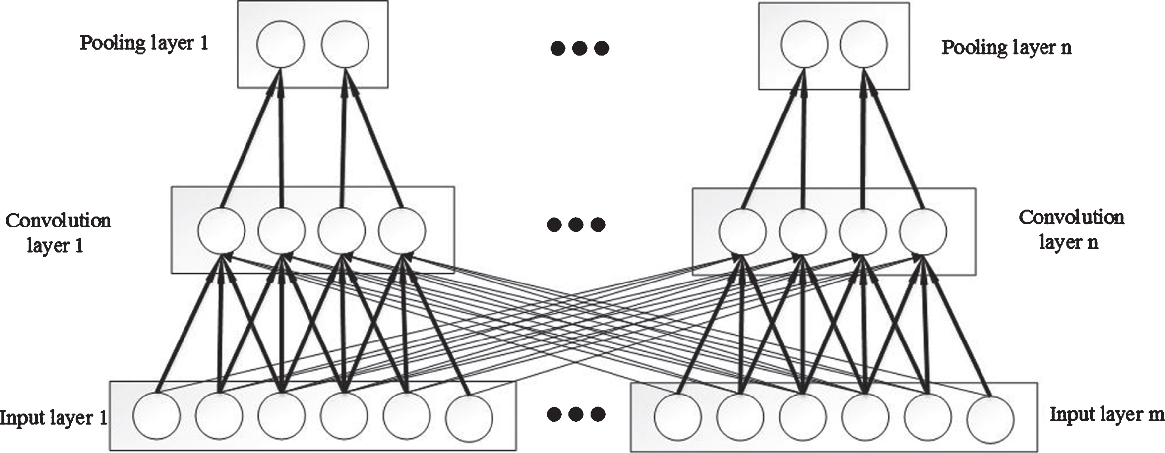
The structural sketches of 1D CNN [13].

Where $x_{ij}^{l}$ is the input of the l^th convolutional layer; $y_{ij}^{l}$ is the output from the l^th convolutional layer; $b_{j}^{l}$ represents the bias for the j^th feature map, w is the weight of the kernel, m is the index value of filter.

3.2 Long short-term memory

Recurrent Neural Network (RNN) has been widely used in speech recognition, language modeling, video processing and other fields. With the increase of time series, gradient disappearance or explosion will happen while training the traditional RNN network. Therefore, researchers proposed LSTM [14] model. LSTM introduces gate mechanism which consists of an input gate, an output gate and a forget gate (Fig. 2). Gate mechanism solves the problem of gradient dispersion in RNN and the long-term dependencies in the data. 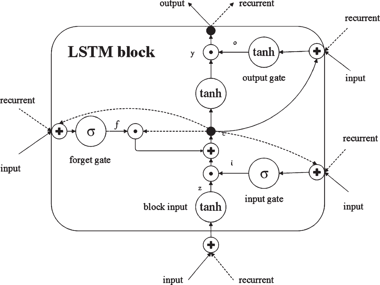The formula derivation of LSTM is illustrated in Equations (2)–(7): $f_{t} = σ (W_{f} \cdot [h_{t - 1}, X_{t}] + b_{f})$ (2) $i_{t} = σ (W_{i} \cdot [h_{t - 1}, X_{t}] + b_{i})$ (3) ${\tilde{C}}_{t} = tanh (W_{C} \cdot [h_{t - 1}, X_{t}] + b_{C})$ (4) $C_{t} = f_{t} * C_{t - 1} + i_{t} * {\tilde{C}}_{t}$ (5) $O_{t} = σ (W_{o} \cdot [h_{t - 1}, X_{t}] + b_{o})$ (6) $h_{t} = O_{t} * tanh (C_{t})$ (7)

Fig. 2

The schematic of LSTM [7].

Where W_f, W_i, W_c and W_o are input weights; b_f, b_i, b_f and b_o are bias weights; h_t is the outputs; x_t is the input; f_t is the output of forget gate; i_t is the output of input gate; O_t is the output of output gate; C_t is the cell state, which represents the specific value of a cell at a certain time. It is the only transfer variable between different times, determined by the state of all previous cells and the current input. ‘*’ represents convolution. The σ is sigmoid function, as shown in Equation (8). The tanh is shown in Equation (9). $sigmoid (x) = \frac{1}{1 + e^{- x}}$ (8) $tanh (x) = \frac{e^{x} - e^{- x}}{e^{x} + e^{- x}}$ (9)

3.3 Batch normalization

There are some problems still exist during the training of deep neural networks. For example, a small change of the parameters in one layer may have significant impacts on the outputs of all the following layers because of the large number of layers. Frequent parameter modification will debase the training speed of the deep neural networks. In addition, it will cause data fall into the range that activation function is insensitive, which will make model training failure. To solve these problems, batch normalization (BN) [15] has been proposed, which can make full use of neurons in deep network. By centralizing and standardizing the input of each layer, BN layer can effectively improve the speed and accuracy of network training. The formulas of batch normalization are shown in Equation (10)–(13): operation which conducted by convolution core [11, 12]. $μ_{B} = \frac{1}{m} \sum_{i = 1}^{m} x_{i}$ (10) $σ_{B}^{2} = \frac{1}{m} \sum_{i = 1}^{m} (x_{i} - μ_{B})^{2}$ (11) $x_{i} = \frac{x_{i} - μ_{B}}{\sqrt{σ_{B}^{2} + ɛ}}$ (12) $y_{i} = γ x_{i} + β \equiv {BN}_{γ, β} (x_{i})$ (13)

Where x_i is the input value and y_i is the output after batch normalization; m is the mean of the mini-batch size; μ_B refers to all the inputs in the same mini-batch; and $σ_{B}^{2}$ is the variance of the input in a mini-batch. To obtain y_i, by the values of μ_B and $σ_{B}^{2}$ , all the x_i are normalized as $\hat{x_{l}}$ and replace by Equation (13). γ and β can adjust the x_i slightly.

3.4 Dropout

To reduce overfitting effectively, dropout was introduced by Hinton [16]. Neurons will be inactivated with probability p when dropout be used (Fig. 3) and the model will not depend too much on local features and specific network structure, which will enhance the generalization ability of the model. Dropout can force the network to be accurate even in the absence of certain information.

Fig. 3

Neural network using dropout.

3.5 Convolutional-LSTM

For predicting NOx emission in FCC unit, the proposed CLSTM model is shown in Fig. 4. The architecture consists of three parts: (1) two layers of CNN; (2) an LSTM layer; and (3) three full connected (FC) layers. Detailed descriptions of these three parts are as following.

Fig. 4

The architecture of proposed CLSTM.

3.5.1 CNN layer

Two convolution parts (Conv in Fig. 4) are used as the CNN layer of the network structure. The first CNN layer contains 16 kernels of size 1*5, the second layer contains 32 kernels of size 1*5. Each convolutional layer is followed by a ReLU layer in Equation (14) and a max pooling layer. BN is added to the convolutional layer. The outputs of the second CNN part are reshaped to 32-dimensional vector. All the vectors form a sequence and feed into the LSTM layer which will be described in next section. $a_{i, j, k} = max (z_{i, j, k}, 0)$ (14)

Where z_i,j,k is the input of the activation function at location (i, j) on the k^th channel. ReLU allows the neural networks to compute faster than sigmoid or tanh activation function. By using ReLU, deep neural networks can be trained efficiently [17].

3.5.2 LSTM layer

In this layer, we employ the same LSTM structure as described in [14]. With the incorporation of the LSTM network, the proposed convolutional-LSTM network can be trained with multivariate time series data of FCC unit. The output of the LSTM layer in this approach is a sequence of 50 dimensional vectors.

3.5.3 Dropout and full-connected layer

The features extracted from the CNN layer are imported into two FC layers. The dropout layers randomly remove connections between CNN layer and FC layer in each iteration to and enhance the generalization ability. In this experiment, the probability has been set to 0.25.

4 Experiments

4.1 Data preparation

The different dimensions will affect the results of data analysis, so it is inappropriate to use the initial data in the training of CLSTM. Data preprocessing consists of the following steps.

4.1.1 Data standardization

In order to eliminate the influence of different dimensions, data standardization is conducted to process initial data. In this paper, Min Max Scaler is used to standardize data as shown in Equation (15-16): $X_{std} = \frac{X - X_{._{min}}}{X_{._{max}} - X_{._{min}}}$ (15) $X_{scaled} = \frac{X_{std}}{(max - min) + min}$ (16) where X_max and X_minare the maximum and minimum values in the data, max and min are the maximum and minimum values of each dimension data.

4.1.2 Transform data into supervised learning

Data must be converted into the supervised learning dataset in time series forecasting problems. We divide the time series into input (x) and output (y) using lag time method, and specifically, in the paper we have used different sizes of lag from 1 to 12.

4.1.3 Divide data into training set and test set

The data was divided into two datasets with training data and verification data. The models were trained with 70% of the observation data and verified with 30% of the observation data.

4.2 Performance criteria

The statistical measures used for comparing the model performance are the mean absolute error (MAE) [18], the root mean square error (RMSE) [19], Pearson correlation coefficient (PCCS) and coefficient of determination (R2). MAE in Equation (17) represents the mean value of absolute error between the predicted value and the observed value. It can avoid mutual cancellation of errors, and accurately reflect the size of actual prediction error. $MAE = \frac{1}{N} \sum_{n = 1}^{N} | o_{n} - p_{n} |$ (17)

RMSE reflects the deviation between predicted and observed values, the formula of RMSE is shown in Equation (18): $RMSE = \sqrt{\frac{\sum_{n = 1}^{N} {(o_{n} - p_{n})}^{2}}{N}}$ (18)

PCCS is used to measure the correlation between two variables. Its value is between -1 and 1. The greater the value of PCCS, the stronger the correlation. The formula of PCCS is shown in Equation (19):

$r = \frac{\sum_{n = 1}^{N} o_{n} - \sum_{n = 1}^{N} o_{n} \sum_{n = 1}^{N} p_{n}}{\sqrt{N \sum_{n = 1}^{N} o_{n}^{2} - {(\sum_{n = 1}^{N} o_{n})}^{2}} \sqrt{N \sum_{n = 1}^{N} p_{n}^{2} - {(\sum_{n = 1}^{N} p_{n})}^{2}}}$ (19)

for Equations (14), (15) and (16), N is the length of the data. o_n is mean of observed values and p_n is mean of predicted values.

The R² reflects the fitting degree of the model. The formula of coefficient of determination is shown in Equation (20): $R^{2} = \frac{SSR}{SST} = \frac{\sum_{i = 1}^{n} {(p_{n} - \bar{o_{n}})}^{2}}{\sum_{i = 1}^{n} {(o_{n} - \bar{o_{n}})}^{2}}$ (20)

Where SSR refers to regression sum of squares, SST refers to total sum of squares. p_n is mean of predicted values. $\bar{o_{n}}$ is average value, and o_n is the observed values.

4.3 Performance comparisons

To prove the validity of the proposed CLSTM model for NOx emission in FCC unit. We conducted experiments using CNN, SVM [20, 21], MLP, RF [22, 23] LSTM. Models run 10 times to avoid the occasionality. The inputs of models are the concentration of NOx emission and other factors that can affect the NOx emission (i.e., material quantity, temperature of flue gas, temperature of dense bed and main air flow). The outputs are the NOx emission concentration of the next hours.

In the training process of CLSTM model, Adaptive Moment Estimation (Adam) [24] is used as the optimization algorithm. Adam obtains the advantages of Adaptive subgradient (AdaGrad) [25] and Root Mean Square Prop (RMSProp) [26]. Table 1 shows the concrete setting of the other models. The evaluation of different methods includes three aspects.

Table 1
Parameters for machine learning methods

# Model Description

1 SVM kernel = “linear”, C = 40

2 MLP input_dim = 180, units = 360

3 RF n_estimators = 1000, n_jobs = –1

4 LSTM input_dim = 50, optimizer = ’adam’

#	Model	Description
1	SVM	kernel = “linear”, C = 40
2	MLP	input_dim = 180, units = 360
3	RF	n_estimators = 1000, n_jobs = –1
4	LSTM	input_dim = 50, optimizer = ’adam’

4.3.1 Statistical measures

Figure 5 includes the performance of 10 experiments of machine learning models. SVM, MLP, RF, LSTM are adopted for comparison. Table 2 shows the average of 10 experiments. We have compared the statistical measures with the classical machine learning models in Fig. 5 and Table 2. By analyzing these statistical measures, we can conclude that the excellent performance of 16.8267 MAE, 23.7089 RMSE, 0.9263 PCCS and 0.8237 R2 in CLSTM.

Fig. 5

The Statistical measures of 10 experiments.

Table 2

Performance comparison of machine of machine learning

Method	MAE	RMSE	PCCS	R²
CNN	63.7723	83.7962	0.5153	0.3224
MLP	27.2224	32.9779	0.9122	0.6607
RF	24.9023	31.8688	0.8840	0.6801
LSTM	18.6061	26.2065	0.9228	0.7663
SVM	17.7096	24.1980	0.9166	0.7678
CLSTM	16.8267	23.7089	0.9263	0.8237

4.3.2 Residual graph

Figure 6 shows the residual graphs of all machine learning models in this paper. Residual graphs are used to estimate whether the residual of the predicted value is consistent with the random error [27], and it should not contain any interpretable and predictable information in residual. The residuals of the predicted and observed values are taken as ordinates and the predict values as abscissas. As we can see, in the whole range of abscissa, only the points on the residual graph of the proposed CLTM model are evenly spread on both sides of 0, although there are a few points with irregular distribution. The distribution of residuals effectively reflects the randomness and unpredictability. It indicates that CLSTM can fully capture the predictable information in the data of NOx emission.

Fig. 6

The residual graph of machine learning models.

4.3.3 Predicted results graph

As the information belonging to the enterprise internal data, we intercepted a part of the prediction results and scale the values, which is shown in Fig. 7 The green curves refer to the observed value and the red curves represent the predicted value. As we can see that the proposed CLTM model achieves high performance at both global and local time periods.

Fig. 7

The predicted results graph of machine learning models.

5 Conclusion

In this paper, the CLSTM model have been proposed for forecasting of NOx emission in FCC unit. The difficulties in predicting NOx emission in FCC lie in the properties of data with multivariate time series. The proposed CLSTM model accurately predicts NOx emission in FCC unit with low computational costs which benefit by the extraction ability of CNN between different sequences. The accuracy of CLSTM is further enhanced by the inclusion of LSTM layer. We compared the CLTM model with the classical machine learning models such as CNN, MLP, RF, SVM and LSTM. Better performance was achieved from CLSTM than that from the classical machine learning models. On the other hand, the CLSTM model relies on large efforts to determine the optimal hyperparameters. Although there are some methods to solve this problem, it is still a limitation of CLSTM. Future works include eliminate the influence of noise and effectively feature extracting in the CNN layers.

Footnotes

Acknowledgments

The authors would like to thank the associated editors and the reviewers for their precious time and efforts in reviewing our paper and providing constructive comments to improve the paper. This work was supported by Science Foundation of China University of Petroleum-Beijing under grant No. 2462018YJRC007, Research on Prediction and Early Warning System of Air Pollution Emission in Catalytic Fracture Device and New Control Model” under grant No. 2017D-5008.

References

, Zeng

L.K.

, Wang

and Cheng

X.S.

, Technological Feasibility for Controlling NOx Emission of Ceramic Furnace, Chinese Academy of Sciences 22(3) (2015), 35–42.

Lin

J.L.

, Hua

X.B.

, Wu

Y.Q.

and Yang

, Generation and Control of Nitrogen Oxides in Flue Gas of Catalytic Plant Regeneration, Environmental Protection in Petrochemical Industry 28(1) (2005), 34–38.

Zafra

, Angel

and Torres

, ARIMA ananlysis of the effect of land surface coverage on PM10 concentrations in a high-altitude megacity [J], Atmos Pollut 8 (2017), 660–668.

Orbach

, Principles of Neurodynamics, Perceptrons and the Theory of Brain Mechanisms Arch Gen Psychiatry 7 (1962), 218.

Krizhevsky

, Sutskever

and Hinton

G.E.

, ImageNet Classification with Deep Convolutional Neural Networks, In Lake Tahoe, NV, USA, Proceedings of the 25th International Conference on Neural Information Processing Systems (NIPS) 3–6 (2012), 1097–1105.

Hochreiter

and Schmidhuber

, Long Short-Term Memory, Neural Comput 9 (1997), 1735–1780.

Greff

, Srivastava

R.K.

, Koutnik

, Steunerbrink

B.R.

and Schmidhuber

, LSTM: A Search Space Odyssey, IEEE Trans Neural NETW Learn Syst 28 (2017), 2222–2232.

Ding

and Pang.

, A deep hybrid learning model to detect unsafe behavior: Integrating convolution neural networks and long short-term memory, Automation in Construction 86 (2018), 118–124.

Huang

C.-J.

and Kuo

P.-H.

, A deep CNN-LSTM model for particulate matter (PM2.5) forecasting in smart cities, sensors (2018).

10.

Downie

, Le Calvez

J.H.

and Kerrihard

, Real-Time microseismic monitoring of simultaneous hydraulic fracturing treatments in adiacent horizontal wells in the woodford shale, Frontiers+innovation 2009 CSPG CSEG CWLS convention 26 (2009), 484–492.

11.

Le Cun

, Bottou

and Bengio

, Gradient-based learning applied to document recognition, Proceedings of the IEEE 86(11) (1998), 2278–2324.

12.

Li-Gang

, Pai-Yu

and Shi-Meng

, Demonstration of convolution kernel operation on resistive cross-point array, IEEE Electron Device Letters 37(7) (2016), 870–873.

13.

Fei-Yan

, Lin-Peng

and Jun

, Review of Convolutional Neural Network, Chinese Journal of Computers 40(2) (2017).

14.

Dunea

, Pohoata

and Iordache

, Using wavelet-feedforward neural networks to improve air pollution forecasting in urban environments, Environ Monit Assess 187 (2015), 477.

15.

Ioffe

and Szegedy

, Batch Normalization: Accelerating Deep Network Training by Reducing Internal Covariate Shift, In, Proceedings of the 32nd International Conference on International Conference on Machine Learning, Lille, France, 6–11 37 (2015), 448–456.

16.

Hinton

G.E.

, Srivastava

, Krizhvsky

, Sutskever

and Salakhutdinov

R.R.

, Improving neural networks by prenventing co-adaptation of feature detectors, CoRR abs/1207.0580.

17.

Dan Foresee

and Hagan

M.T.

, Gauss-Newton approximation to Bayesian learning. In Proceedings of the IEEE International Conference on Neural Networks, Houston, TX, USA, 2 June 1997; IEEE: Piscataway, NJ, USA, (1997), 3 1930–1935.

18.

Zhang

, Mean-Mean Absolute Deviation Portfolio Model and Optimization, Statistics and Decision-Making 2009(1), 14–15.

19.

, Li

and Ji

J.H.

, Statistical Basis (2nd Edition), Machinery Industry Press, (2016).

20.

Das

and Akpinar

, Investigation of Pear Drying Performance by Different Methods and Regression of Convective Heat Transfer Coefficient with Support Vector Machine, Appl Sci 8 (2018), 215.

21.

Liu

J.P.

and Li

C.L.

, The short-term power load forecasting based on sperm whale algorithm and wavelet least square support vector machine with DWT-IR for feature selection, Subtainability 9 (2017), 1188.

22.

, Qiao

, Hu

, Huang

, Sangaiah

A.K.

, Zhang

, Wang

and Zhang

, De-Anonymizing Social Networks With Random Forest Classifier, IEEE Access 6 (2018), 10139–10150.

23.

Zhu

, Xia

, Jin

, Yan

, Cai

and Yan

, Class Weights Random Forest Algorithm for Processing Class Imbalanced Medical Data, IEEE Access 6 (2018), 4641–4652.

24.

Kingma

D.P.

and Ba

, Adam: A method for stochastic optimization, Proc ICLR (2015).

25.

Duchi

, Haza

and Singer

, Adaptive subgradient methods for online learning and stochastic optimization, Journal of Machine Learning Research 12(Jul) (2011), 2121–2159.

26.

Riedmiller

and Braun

, RPROP-A fast adaptive learning algorithm, Proc. ISCIS, (1992).

27.

Xue

and Chen

L.P.

, Practical Data Analysis and MATLAB Software, Beijing University of Technology Press, (2015).