Hybrid deep learning models based emotion recognition with speech signals

Abstract

Emotion recognition is one of the most important components of human-computer interaction, and it is something that can be performed with the use of voice signals. It is not possible to optimise the process of feature extraction as well as the classification process at the same time while utilising conventional approaches. Research is increasingly focusing on many different types of “deep learning” in an effort to discover a solution to these difficulties. In today’s modern world, the practise of applying deep learning algorithms to categorization problems is becoming increasingly important. However, the advantages available in one model is not available in another model. This limits the practical feasibility of such approaches. The main objective of this work is to explore the possibility of hybrid deep learning models for speech signal-based emotion identification. Two methods are explored in this work: CNN and CNN-LSTM. The first model is the conventional one and the second is the hybrid model. TESS database is used for the experiments and the results are analysed in terms of various accuracy measures. An average accuracy of 97% for CNN and 98% for CNN-LSTM is achieved with these models.

Keywords

Machine-learning Deep learning CNN LSTM

1. Introduction

The ability to comprehend and respond to human feelings is essential to successful human-machine interaction. Humans can hide their expressions in faces easily at that time it is difficult to find accurate emotions in such cases speech signals are very helpful and it is difficult to hide their voices compared to the face. Speech is the most straightforward and effective method of communication available to humans. Emotion identification through the analysis of speech signals has many potential uses, including in contact centres, classrooms, lie detectors, security systems, healthcare, video games, and more [1]. There are two primary components to any speech emotion detection system: feature extraction from speech signals and classification of those features according to emotional states [2]. A wide variety of speech parameters, including pitch [3], zero crossing rate, formants, signal energy [4], maximum amplitude, Mel Frequency Cepstral Coefficients (MFCC), etc. [5], are employed in speech analysis. After features are extracted, they are fed into a classifier like a Gaussian Mixture Model (GMM) [8, 9], Support Vector Machine (SVM) [6, 7], a Decision Tree [8, 10], a Bayesian Network model [9], or a Nearest Neighbor [10].

Researchers are focusing more of their time and energy on Deep Learning methods currently. When confronted with a problem, deep learning algorithms use a comprehensive learning cycle. In the subject of emotion recognition from audio signals, two of the most current approaches to be employed are convolutional neural networks and long short term memory networks. These two methods are addressed as being among the most recent methods used. Emotional speech can be recognised using either a one-dimensional or a two-dimensional CNN-LSTM model, both of which are described in [11]. The IEMOCAP and Berlin EmoDB public databases served as the experimental platforms. The outcomes demonstrate that 2D CNN-LSTM outperforms its 1D counterpart. Following the high-level feature extraction performed by Convolutional layers, the LSTM model is utilised to hold long-term dependencies, and finally, two dense layers round up the CNN+LSTM architecture suggested in [12]. The SAVEE database was used to conduct the study. Emotional speech identification based on spectrograms is explored in [13]. Here, the Spectrograms are fed into a CNN model. The following chapters constitute the various parts of this investigation. Following an explanation of the database in Section 2, which is followed by explanations of the architectures of Convolutional Neural Networks (CNN’s) and Long Short Term Memory Networks- (LSTM’s) in Sections 3 and 4, Section 5 describes the models used in this work for speech emotion recognition, which are CNN and CNN-LSTM, Section 6 discusses the investigational results, Section 7 is a Comparative analysis, and Section 8 is the Conclusion. Section 1 is an introduction to the database.

2. Database

Toronto Emotional Speech Set (TESS) was established to study how ageing affects emotion perception. Two female actresses – 60 and 20 – comprise this dataset. Each actor simulated seven emotions for 200 neutral sentences. This dataset includes disgusted, angry, neutral, delighted, astonished, terrified, and sad. 56 undergraduates were asked to label the dataset by recognising emotions from utterances. The dataset comprised utterances with over 66% confidence after the identification exercise. TESS is at https://tspace. library.utoronto.ca/handle/1807/24487.

3. Convolutional Neural Networks (CNN)

3.1 CNN: An overview

The Convolutional Neural Network (CNN) is widely regarded as one of the most significant models for deep learning. CNNs have been demonstrated to be useful in a wide variety of contexts, including the categorization of text, the investigation of documents, computer vision, object detection, and the processing of images. The convolution stage, the pooling stage, and the fully connected layer are the three fundamental building layers that are utilised in convolution neural networks, as described in [14]. These stages are respectively the convolution stage, the pooling stage, and the fully connected layer. Figure 1 presents a diagram of the primary CNN’s underlying architecture.

Figure 1.

Architecture of Simple CNN.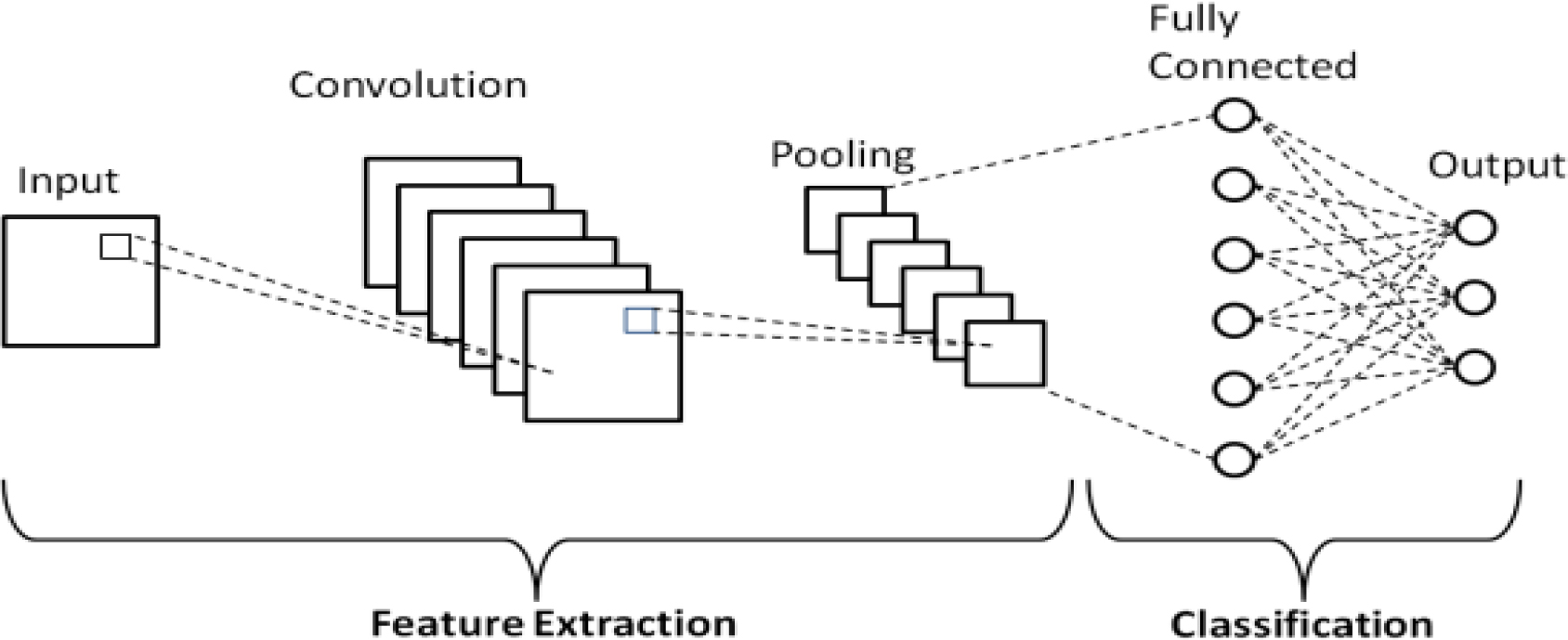

3.2 Convolutional Layer (CL)

The Convolutional Layer (CL) is an essential component in the construction of neural networks. The function of feature extraction is carried out by the convolution layer in a CNN design. In order to extract, one uses the helpful characteristics that are found in the convolution layer of the inputs. The technique of convolution consists of doing nothing more complicated than applying a filter to the input in order to generate activation. When the same filter is used multiple times, a type of map of activations known as a feature map is produced. The formation of these feature maps is accomplished by passing incoming data through a number of different filters. The 1D and 2D convolution processes are illustrated respectively in Figs 2 and 3, respectively.

Figure 2.

1D Convolution operation of n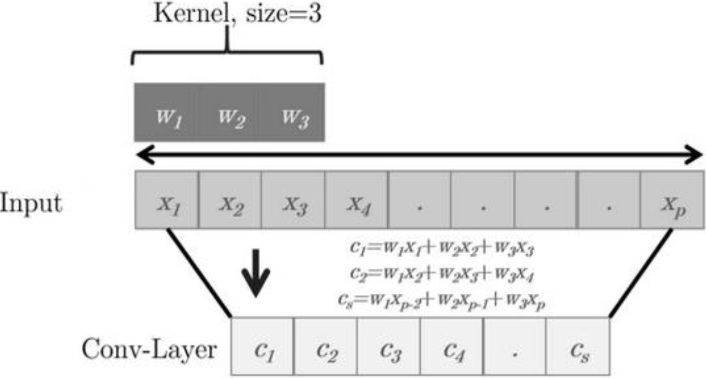 $\times$ 1 matrix with 3 $\times$ 1 filter.

Figure 3.

Convolution in two dimensions performed on a 5 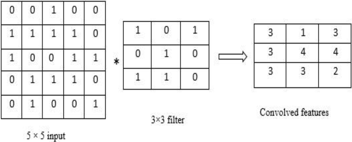$\times$ 5 matrix using a 3 $\times$ 3 filter.

3.3 Pooling Layers (PL)

The pooling layer’s purpose is to cut down on the size of the convolved features as much as possible. Just taking into account the information that is most relevant to the problem at hand will cut down on the amount of computation that is required to progress the data. Two common strategies for pooling data are the maximum pooling and the average pooling. The Max pooling method is employed to obtain the segment with the biggest value, and the Average pooling procedure is utilised to acquire the segment with the values that are representative of the segment on average. Figures 4 and 5 illustrate an example of maximum and average pooling in both a one-dimensional and a two-dimensional setting, respectively.

Figure 4.

1D max and average pool operations with pooling size 2.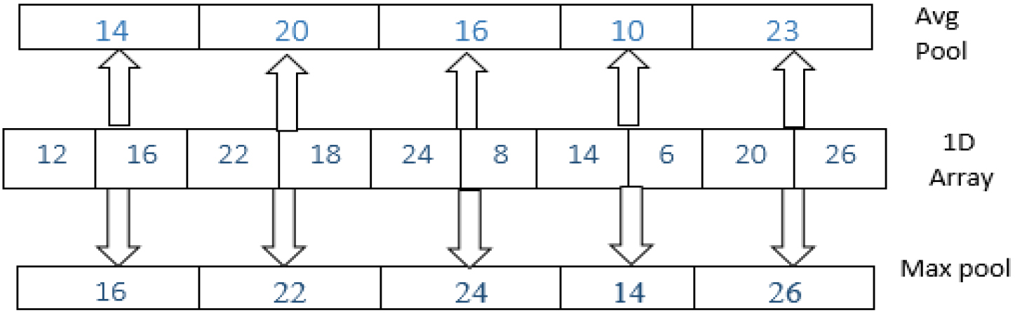

Figure 5.

2D pooling with stride 2.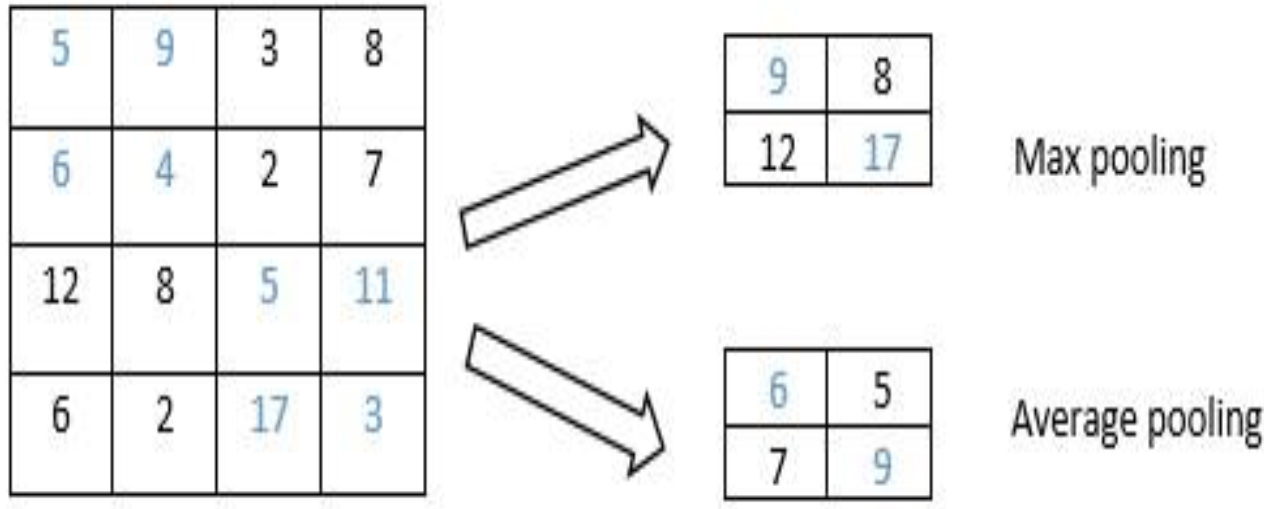

3.4 Fully Connected Layer (FCL)

It creates a 1D array by mixing the inputs from the layers that came before it. The number of classes serves as the determinant for the output dimensions. Figure 6 is the example of a small fully-connected layer with four input and eight output neurons.

Figure 6.

Fully Connected layer.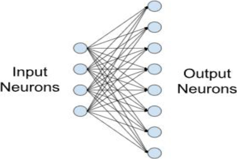

3.5 ReLU Layer (ReLU)

The word that is used is “rectified linear unit,” also written as “ReLU.” Once the feature maps have been collected, they need to be imported into a ReLU layer for further processing. The process of cancelling out all of the negative pixels in an image is carried out by ReLU in a step-by-step manner. As a consequence of the network changing into a non-linear structure, a rectified feature map is generated [15]. The graph of a ReLU function is presented here in Fig. 7.

Figure 7.

ReLU function.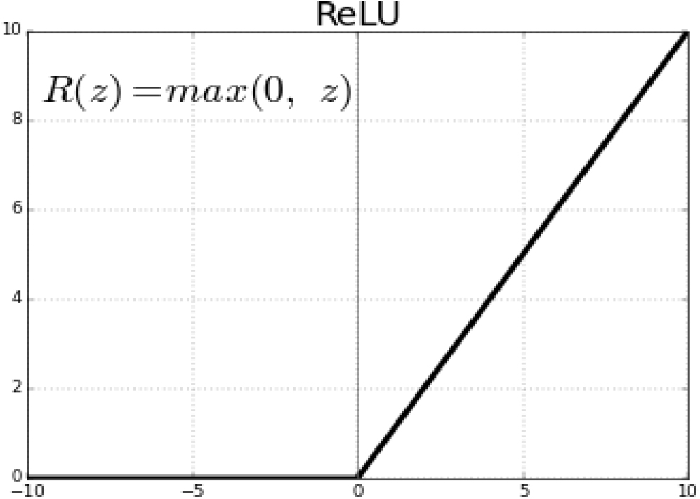

Figure 8.

a) Without Dropout; b) With Dropout.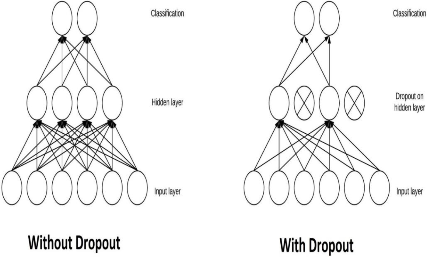

3.6 Dropout Layer (DL)

Dropout is a method of regularisation for neural networks that helps to mitigate the effects of overfitting [16]. As shown in Fig. 8, Dropout takes random samples from a Bernoulli distribution and zeroes out part of the connections of the input tensor with a probability $p$ . This process is carried out in a random manner.

Figure 9.

Softmax activation.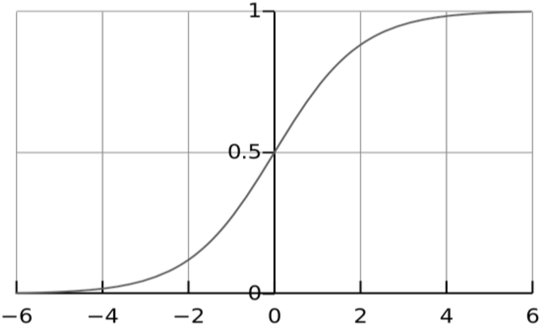

3.7 Softmax Function (SF)

The softmax function can also be referred to by its alternate name, softargmax. This function’s objective is to normalise the output of neural networks so that it falls somewhere in the range of 0 and 1, as specified in [17]. The graphic depiction of the softmax function can be seen in Fig. 9, which can be seen below.

The formula for the SF is given below.

$\displaystyle\text{Softmax}(x_{i})=\frac{{\exp}\left({x_{i}}\right)}{\sum_{j}% \exp\left({x_{j}}\right)}$ (1)

The value of Softmax is calculated by taking the exponent of each individual input vector and dividing that number by the total exponents for all of the inputs.

3.8 Loss Function (LF)

It measures how well a model fits data. If forecasts differ from goal values, the loss function number will be higher. If not, it will be lower. CNN’s Cross Entropy Loss Function checks the model’s reliability after applying the Softmax Function [18]. This optimises neural network performance. Figure 10 shows that when the expected probability falls, the log loss (entropy loss) increases quickly.

Figure 10.

Loss function graphical representation.

The formula for the Loss function is given below.

$\displaystyle H\left({p,q}\right)=-\mathop{\sum}\nolimits_{x}q\left(x\right)% \log p\left(x\right)$ (2)

True and approximated distributions are $p(x)$ and $q(x)$ .

4. Long Short Term based Memory Networks (LSTMN)

Long-term data storage is possible with the complicated RNN LSTM. Data determines whether the network keeps memory. Gating maintains the network’s long-term dependencies [19]. Network gating allows memory release or retention. LSTM cells have three gates. Figure 11 shows that the Forget gate comes first, followed by the Input and Output gates.

Figure 11.

Cell of LSTM with gates.

Figure 12.

LSTM Cell states.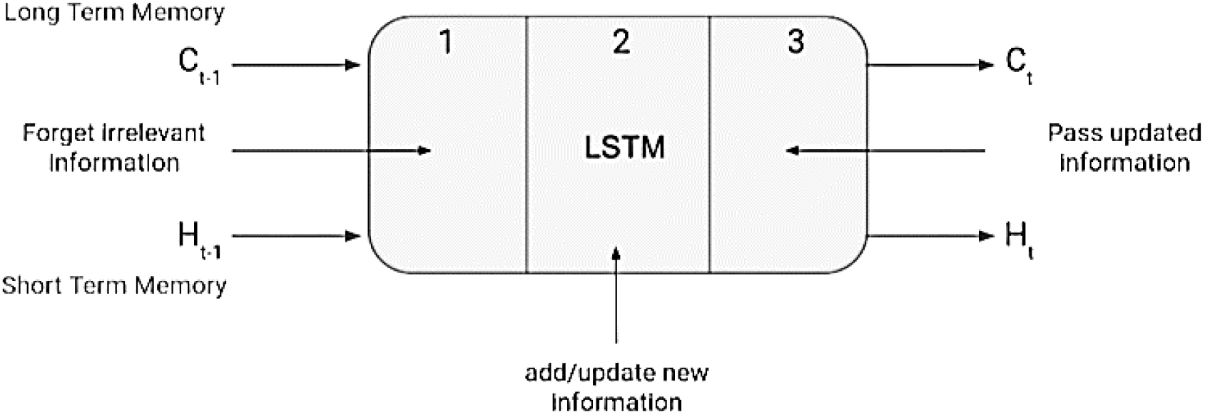

Figure 13.

Working of LSTM cell.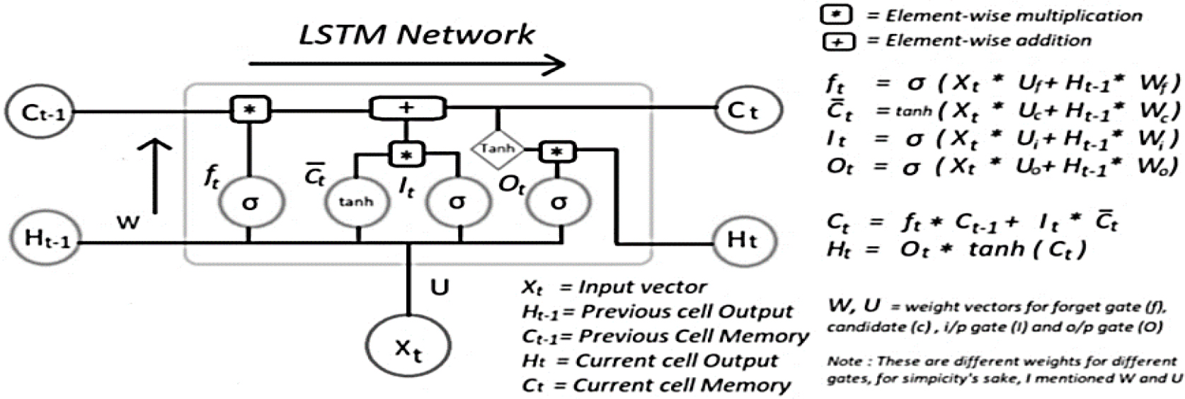

The hidden state of an LSTM, which is identical to a simple RNN, is $H(t-1)$ from the timestamp before the current one and Ht from the current one. As seen in Fig. 12, LSTMs have a cell state, denoted by $C(t-1)$ and $C(t)$ for past and present timestamps.

Under the parameters of this discussion, both the concealed state and the cell state are associated with short-term memory. The LSTM operation is broken down into its basic steps and depicted in Fig. 13.

Forget gate: The series of gates begins with the forgetting gate as the initial barrier. If you exit the application, none of the memories you’ve created with it will be saved. It is possible that if you open this gate all the way, you will be able to release some of the memories from your past. In point of fact, it’s just a multiplication of the individual components that make up the whole. In case you lapsed into forgetfulness, the equation for the forget gate is as follows:

$\displaystyle f_{t}=\sigma\left({U_{f}\ast X_{t}+W_{f}\ast H_{t-1}\ast}\right)$ (3)

When you multiply something by a vector that is somewhat near to zero, you are working towards the goal of erasing the memory of what came before. Adjust the forget gate such that it is set to 1 to let the old memories pass through.

$\displaystyle f_{t}\ast C_{t-1}=0\ \ \textit{if}\ \ f_{t}=0$ (4) $\displaystyle f_{t}\ast C_{t-1}=C_{t-1}\ \ \textit{if}\ \ f_{t}=1$ (5)

Where $X_{t}$ is a representation of the input for the current time stamp and $H(t-1)$ is a representation of the hidden state of the time stamp, respectively. The weights that correspond to the input state, denoted by the notation $U_{f}$ , and the concealed state are denoted by the notation $W_{f}$ .

Input gate: The circuit has two gates total, and the second gate is the input gate. The second gate defines the maximum quantity of extra input that should be permitted and acts as a cap on the total amount of input. There should be a difference in the effect that this gate has on fresh memories and old memories if this gate is adjusted properly. The relevance of the data that is being carried by the input is evaluated by the input gate in order to determine how recent the data is. The function of the input gate can be characterised using the following equation:

$\displaystyle i_{t}=\sigma\left({X_{t}\ast U_{i}+H_{t-1}\ast W_{i}}\right)$ (6)

Where $U_{i}$ and $W_{i}$ are the weights that correspond to the currently available input and the previously hidden states, respectively.

Cell State: The plus sign comes next in this list. The operation known as piecewise summation is what this operator is defined as. This action will integrate the most recent input with the previously stored data in the memory. For the purpose of generating St., this is the element-wise sum of the current input and the previous memory.

$\displaystyle{\bar{C}_{t}}=\textit{tanh}(U_{c}\ast X_{t}+\ast W_{c}\ast H_{t-1% })\ (\text{Newly Added information})$ (7) $\displaystyle C_{t}=C_{t-1}\ast f_{t}\ast+I_{t}\ast\bar{C}_{t}\ (\text{% Updatation of cell state})$ (8)

Output gate: It is necessary to have it in order to generate the output of this LSTM. At this level, the output gate is managed by a combination of the new memory, the current input, and the output from the level before it. At this level, the output gate was managed by just the current input. This gate is responsible for determining the proportion of the freshly produced memory that should be sent on to the LSTM unit that follows it.

$\displaystyle O_{t}=\sigma\left({X_{t}\ast U_{O}+H_{t-1}\ast W_{O}}\right)$ (9)

The sigmoid function guarantees a 0 to 1 output value. We’ll utilise the modified cell states in the following equation to find the hidden state. This will reveal the hidden state.

$\displaystyle H_{t}=\textit{tanh}\left({C_{t}}\right)\ast O_{t}$ (10)

Long-term memory ( $C_{t}$ ) and current output determine the concealed state. Call SoftMax to activate the hidden state $H_{t}$ and get the current timestamp output. This retrieves output.

$\displaystyle\textit{Output}=\textit{Softmax}(H_{t})$ (11)

5. Architectures used in this study

Voice emotion recognition is the focus of this study, which employs both the CNN and CNN-LSTM neural network designs in its analysis (Convolution neural network – Long short term memory network). The trials were carried out with the help of the TESS dataset.

5.1 CNN architecture

The below is the CNN architecture

•
1 $\times$ Max Pool Layer (MPL) of 8 $\times$ 8 pool size
•
2 $\times$ Convolution Layer (CL) of 256 channel of 8 $\times$ 8 kernel and identical padding
•
1 $\times$ Dense Layer (DL) of 256 units
•
1 $\times$ Dense Softmax Layer (DSL) of 7 unit
•
The ReLU function is used as an activation function in all layers of the network with the exception of the output layer.

Figure 14.
Vector shapes with CNN architecture.

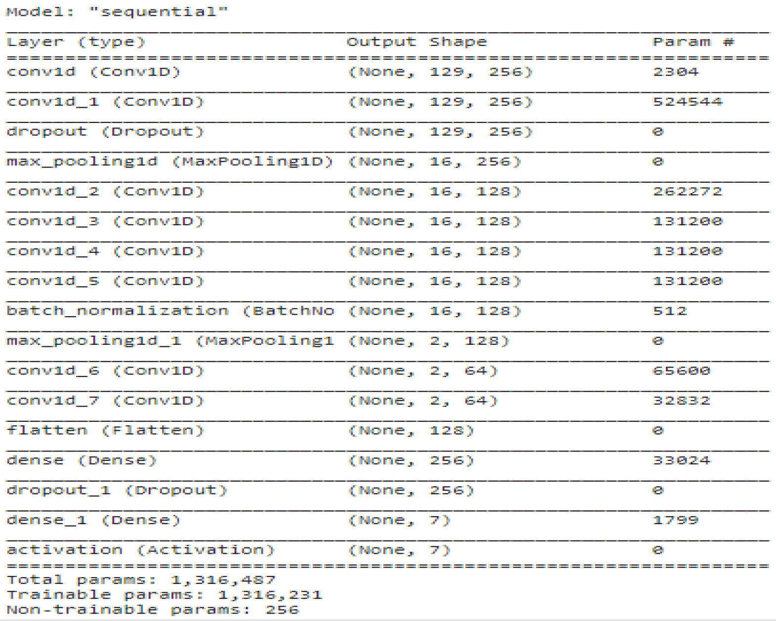
The CNN model’s Keras implementation may be found presented below Table 1 in the following location: This section will provide a deeper dive into the architecture of the CNN, including a discussion of the input and output vector forms that are depicted in Fig. 14.

Table 1
CNN model based Keras implementation

5.2 Architecture of CNN-LSTM

For optimal results in vocal emotion identification, it is recommended to work with a hybrid Convolution LSTM model. The CNN-LSTM model can be broken down into two distinct components with regard to its architecture. The initial step is the production of time series sequential data from the speech stream, followed by the fusion of CNN and LSTM layers. A recurrent neural network, also known as an LSTM, feeds its data back into itself while a convolutional neural network, on the other hand, processes spatial data. A recurrent neural network can also be referred to as an LSTM. The performance of recurrent neural networks is considerably increased when the data is presented in a sequential order. Long short-term memory (LSTM) is able to recognise patterns across time, but convolutional neural networks are only able to recognise patterns in space. The power of this fusion, which takes the best features of both neural networks and integrates them, is not to be under estimated. Figure 15 presents the CNN-LSTM model for your perusal.

Figure 15.

CNN-LSTM ARCHITECHTURE.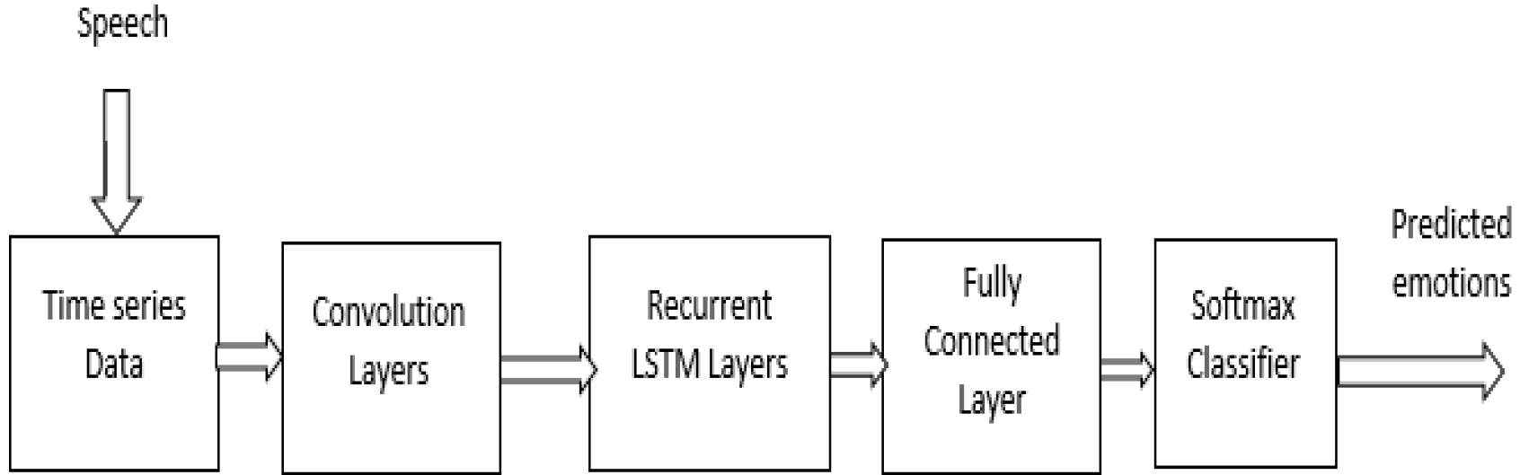

The audio sample is initially converted into a one-dimensional vector, and then it is fed into a one-dimensional network. Convolution layers are utilised in order to discover the regional characteristics of the sample. After being reshaped, the features obtained from the convolution layers are ultimately used as input for an LSTM layer. The characteristics that are derived from the LSTM layer contain both short-term and long-term contextual information that has been incorporated. The completely connected layer (FC) is distinguished by its flattened input, which indicates that each neuron in the layer receives its input from every other neuron in the layer. This is the defining feature of the fully connected layer. In order to prevent over fitting, drop out is inserted after the dense layer. The final layer of this design is referred to as the Softmax classifier, and its function is to classify different emotional states according to the learning properties that they contain. In this particular instance of the model, the categorical cross-entropy serves as the loss function, and the Adam optimizer is the tool that is utilised to locate the best possible answer. Using Google Colaboratory in conjunction with a GPU backend that has 12 gigabytes of Memory was used to carry out the evaluation. The task was accomplished with the help of Google Colaboratory, which included a GPU back end and 12 gigabytes of RAM in its configuration. Using the application programming interfaces provided by Tensorflow and Keras is necessary in order to import the CNN and LSTM layers.

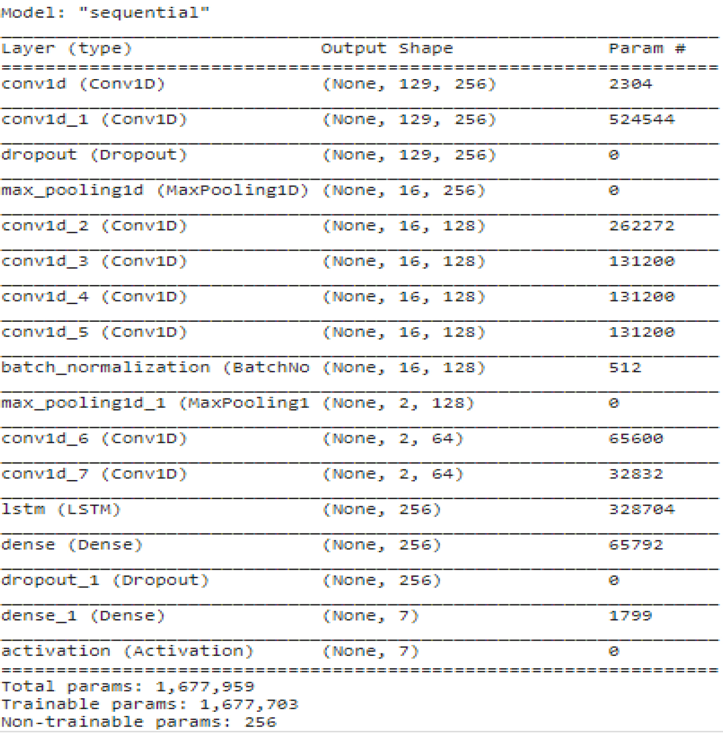
The below is the Structure of the CNN-LSTM model

•

1 $\times$ max pool layer with an 8 $\times$ 8 pool size

•

2 $\times$ Convolution Layers(CL) using the same padding and having 256 channels of the 8 $\times$ 8 kernel

•

4 $\times$ CL using the same padding and having 128 channels of the 8 $\times$ 8 kernel

•

Two layers of convolution, each with 64 channels of an 8 $\times$ 8 kernel and equal padding

•

One layer of maximum pooling, each with an 8 $\times$ 8 pool size

•

256 LSTM internal units comprising the LSTM layer

•

1 layer that is dense with 256 units

•

1 layer that is dense with 7 units of softmax

•

The ReLU activation function can be found throughout the network, with the exception of the output layer, which does not contain this function.

Figure 16.

Vector shapes analysis using CNN-LSTM.

Table 2 shows the CNN-LSTM model that is displayed in the Keras implementation, which can be seen further down on this page. This is a deeper dive into the CNN-LSTM architecture, including a discussion of the input and output vector forms that are depicted in Fig. 16.

Table 2

CNN-LSTM based Keras implementation

6. Experimental evaluations

The subsequent section presents the results of the tests conducted on the numerous models that were used in this investigation. The F1 score, sensitivity, precision, accuracy, and specificity were the markers of performance that were used for this study [21]. The phrases true positive (TP), false positive (FP), false negative (FN), and true negative (TN) are utilised for the purpose of defining metrics (TN).

Where TP $=$ Model predicts positive TN $=$ Model predicts negative FP $=$ Model predicts positive FN $=$ Model predicts negative

A. Accuracy:

One method that can be used to evaluate the precision of a measurement is to take the total number of samples and divide it by the number of correct samples.

$\displaystyle\textit{Accuracy}=\frac{{\textit{TP}}+{\textit{TN}}}{{\textit{FP}% }+{\textit{FN}}+{\textit{TP}}+{\textit{TN}}}$ (12)

B. Sensitivity:

One definition of sensitivity explains it as the proportion of correct diagnoses that are obtained in comparison to the total number of correct diagnoses and erroneous negative results combined.

$\displaystyle\textit{Recall (Sensitivity)}=\frac{{\textit{TP}}}{{\textit{FN}}+% {\textit{TP}}}$ (13)

C. Specificity:

As compared to the total number of true negative cases and false positive cases, the ratio of the number of true negative instances to the total number of true negative cases and false positive cases should be high for a test to be considered to have a high level of specificity.

$\displaystyle\textit{Specificity}=\frac{{\textit{TN}}}{{\textit{FP}}+{\textit{% TN}}}$ (14)

D. Precision:

The proportion of precisely anticipated positive occurrences in relation to the total number of expected positive cases is one way to quantify precision.

$\displaystyle\textit{Precision}=\frac{{\textit{TP}}}{{\textit{TP}}+{\textit{FP% }}}$ (15)

E. F1 Score:

The $F1$ score is determined by taking the participant’s precision score and adding it to their recall score and averaging the two. It is possible to achieve a higher $F1$ score, which will result in more accurate forecasts.

$\displaystyle\textit{F1 Score}=2*\frac{\left({{\textit{Precision}\ast\textit{% Recall}}}\right)}{\left({{\textit{precision}}+{\textit{Recall}}}\right)}$ (16)

6.1 Results comparison with CNN approach

Figure 17 is an illustration of the outcomes of fitting the data, and it is based on the CNN architecture.

Figure 18 depicts a plot of the model’s accuracy vs its loss in terms of accuracy. Both the loss and accuracy values are impacted when the number of epochs in the calculation is altered. In the below graphs $X$ axis represents number of Epochs and $Y$ axis represents Accuracy or loss parameters.

Table 3 contains an illustration of the confusion matrix for the testing data, which includes 280 different samples. In addition, Table 4 presents the performance metrics of the model that were generated making use of the confusion matrix. These metrics may be found in the previous section.

Table 3
CNN based Confusion Matrix (CM)

	Anger	Disgust	Fear	Happy	Neutral	Sad	Surprise
Anger	43	0	0	0	0	0	0
Disgust	0	33	0	0	0	1	0
Fear	0	0	41	2	0	0	0
Happy	0	0	0	39	1	0	1
Neutral	0	0	0	0	35	1	0
Sad	0	0	0	1	1	35	0
Surprise	1	0	0	4	0	1	40

Figure 17.

Analyzing fitting by using CNN.

While determining the accuracy, specificity, and sensitivity of the model, it is necessary to take into account not only true negatives (TN), but also true positives (TP), false positives (FP), and false negatives (FN), in addition to true negatives (TN). True positive is denoted by the letters TP, while false positive is denoted by FP and true negative is shown by TN. The results of the CNN model’s performance evaluations are presented in Table 4.

Table 4

Performance analysis using CNN

	TP	TN	FP	FN	Sensitivity/recall	Specificity	Precision	F1 score	Accuracy
Anger	43	235	2	0	1	0.99	0.95	0.97	0.99
Disgust	33	246	0	1	0.97	1	1	0.98	0.99
Fear	41	236	0	3	0.93	1	1	0.96	0.98
Happy	39	232	7	2	0.95	0.97	0.84	0.88	0.96
Neutral	35	242	2	1	0.97	0.99	0.94	0.95	0.98
Sad	35	241	2	2	0.94	0.99	0.94	0.93	0.98
Surprise	40	234	1	5	0.88	0.99	0.97	0.91	0.97
Average results					0.94	0.99	0.94	0.94	0.97

Table 5

Confusion Matrix (CM) by using CNN-LSTM

	Anger	Disgust	Fear	Happy	Neutral	Sad	Surprise
Anger	42	0	0	0	0	0	1
Disgust	0	34	0	0	0	0	0
Fear	0	0	44	0	0	0	0
Happy	0	0	1	40	0	0	0
Neutral	0	0	0	0	36	0	0
Sad	0	0	0	0	2	35	0
Surprise	0	0	0	2	1	0	42

Figure 18.

Using CNN Accuracy and Loss comparison.

Upon the completion of the aforementioned computations, the $F1$ score for the model was found to be 0.94, and its accuracy was determined to be 97% when utilising the CNN algorithm.

6.2 Performance with CNN-LSTM technique

The results of fitting the data are illustrated in Fig. 19, which uses the CNN-LSTM architecture as its foundation.

Figure 20 displays the accuracy and loss curves, which were generated by employing the CNN-LSTM model.

The confusion matrix for the test data is presented in Table 5. It includes 280 samples representing the seven distinct emotions of anger, disgust, fear, happy, neutral, and sad, as well as surprise.

Table 6
Performance analysis using the CNN-LSTM

	TP	TN	FP	FN	Recall/sensitivity	Specificity	Precision	F1 score	Accuracy
Anger	42	237	0	1	0.97	1	1	0.98	0.99
Disgust	34	246	0	0	1	1	1	1	1
Fear	44	235	1	0	1	0.99	0.97	0.98	0.99
Happy	40	237	2	1	0.97	0.99	0.95	0.95	0.98
Neutral	36	241	3	0	1	0.98	0.92	0.95	0.98
Sad	35	243	0	2	0.94	1	1	0.96	0.99
Surprise	42	234	1	3	0.93	0.99	0.97	0.94	0.98
Average results					0.97	0.99	0.97	0.96	0.98

Table 7

Performance analysis of CNN and CNN-LSTM

S.no	Network	Sensitivity	Specificity	Precision	F1 score	Accuracy
1	CNN	0.94	0.99	0.94	0.94	0.97
2	CNN-LSTM	0.97	0.99	0.97	0.96	0.98

Figure 19.

Results of Fitting by using the CNN-LSTM architecture.

Table 6, which can be seen below, provides an evaluation of the CNN-LSTM model’s performance, which was utilised in this research. The evaluation can be found below.

According to the calculations that were presented earlier, the $F1$ score is currently sitting at 0.96, and the accuracy of the model, as assessed by the CNN-LSTM model, is currently sitting at 98%. Both of these figures can be found above.

7. Comparative studies

The TESS dataset is utilised in this work for the purpose of voice emotion identification. There are a total of 2800 samples included in the speech data set, of which only 280 are chosen for testing. The results that were obtained for the CNN and CNN-LSTM networks are presented in Table 7.

CNNs can recognise patterns in space, but LSTMs do better in time. CNN and LSTM are combined in the CNN-LSTM model. This combo is efficient and more accurate than CNN alone. The following table compares deep learning methods for voice emotion identification.

Table 8
Comparison of proposed study with other existing works

Method	Average accuracy rate (%)
Auto encoder [22]	96
Time distributed CNN LSTM [23]	89
EMD [24]	93
CNN [25]	85
GRU [26]	96

Table 9

Implementation parameters

Model	CNN	CNN-LSTM
Data set	TESS	TESS
Epochs	50	50
Batch size	50	50
Classifier	Softmax	Softmax
Optimizer	Adam	Adam
Loss function	Categorical_crossentropy	Categorical_crossentropy
Dropout	0.5	0.5
Regularization	Batch Normalization	Batch Normalization

Figure 20.

Loss &Accuracy by using CNN-LSTM.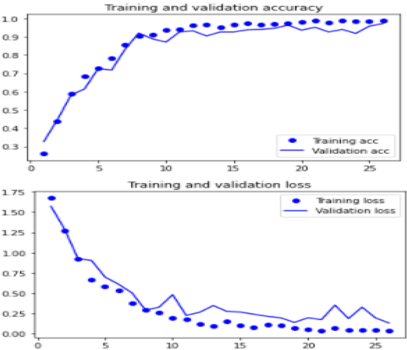

Our CNN-LSTM model achieved the best accuracy, 98%, for the recognition of speech emotions when compared to all of the other research that is currently being carried out.

8. Implementation parameters

The below Table 9 shows some of the implementation parameters for all the two models used in this work. The classifier used for the models is the Softmax classifier and the optimizer is the Adam optimizer and the loss function is categorical cross entropy. The Regularization used for all the models is Batch normalization. And some of the parameters like Dropout, Epoch size, and Batch size are the same for all two models.

9. Conclusions

Both CNN and CNN-LSTM models are utilised in this research for the purpose of speech emotion identification based on the signals produced by the speaker. The architecture used in this work is CNN LSTM. This architecture uses the advantage of both CNN and LSTM. CNNs are powerful for learning local patterns in data, while LSTMs are effective at capturing long-term dependencies in sequential data. Combining these two types of networks can result in improved performance for time series classification tasks. The TESS database served as the testing ground for the experiments. The research were analysed with the help of the TESS database. If you use the CNN model, you will achieve an accuracy of 97%, but if you use the CNN-LSTM model, you will achieve an accuracy of 98%. In contrast to the CNN model, the CNN-LSTM model was successful in achieving a high level of accuracy.

Future Scope: In the present work the CNN-LSTM architecture is tested with speech signals only. In future the model will be developed for EEG and ECG signals also.

References

Lugović

Dunder

Horvat

. Techniques and applications of emotion recognition in speech. In 2016 39th international convention on information and communication technology, electronics and microelectronics (mipro) (pp. 1278-1283). IEEE. 2016 May.

El Ayadi

Kamel

Karray

. Survey on speech emotion recognition: Features, classification schemes, and databases. Pattern Recognition. 2011; 44(3): 572-58.

Ververidis

Kotropoulos

. Emotional speech recognition: Resources, features, and methods. Speech Communication. 2006; 48(9): 1162-1181.

Shete

Patil

. Zero crossing rate and Energy of the Speech Signal of Devanagari Script. IOSR-JVSP. 2014; 4(1): 1-5.

Tiwari

. MFCC and its applications in speaker recognition. International Journal on Emerging Technologies 2010; 1(1): 19-22.

Lin

Wei

. August. Speech emotion recognition based on HMM and SVM. In 2005 international conference on machine learning and cybernetics (Vol. 8, pp. 4898-4901). IEEE. 2005.

Liu

. December. Speaker recognition and speech emotion recognition based on GMM. In 3rd International Conference on Electric and Electronics (EEIC 2013) (pp. 434-436), 2013.

Lee

Mower

Busso

Lee

Narayanan

. Emotion recognition using a hierarchical binary decision tree approach. Speech Communication 2011; 53(9-10): 1162-1171.

Lee

Mower

Busso

Lee

Narayanan

. Emotion recognition using a hierarchical binary decision tree approach. Speech Communication 2011; 53(9-10): 1162-1171.

10.

Sapra

Panwar

. Emotion recognition from speech. International Journal of Emerging Technology and Advanced Engineering 2013; 3(2): 341-345.

11.

Zhao

Yan

Chen

Mao

Wang

Gao

. Deep learning and its applications to machine health monitoring. Mechanical Systems and Signal Processing 2019; 115: 213-237.

12.

Qazi

Kaushik

. A Hybrid Technique using CNN + LSTM for Speech Emotion Recognition.

13.

Badshah

Rahim

Ullah

Ahmad

Muhammad

Lee

Kwon

Baik

. Deep features-based speech emotion recognition for smart affective services. Multimedia Tools and Applications 2019; 78(5): 5571-5589.

14.

O’Shea

Nash

. An introduction to convolutional neural networks. arXiv Preprint arXiv1511.08458; 2015.

15.

Agarap

. Deep learning using rectified linear units (relu). arXiv Preprint arXiv1803.08375, 2018.

16.

Park

Kwak

. November. Analysis on the dropout effect in convolutional neural networks. In Asian conference on computer vision (pp. 189-204); Springer, Cham, 2016.

17.

Liu

Wen

Yang

. Large-margin softmax loss for convolutional neural networks. In ICML (Vol. 2, No. 3, p. 7), 2016 June.

18.

Zhang

Sabuncu

. Generalized cross entropy loss for training deep neural networks with noisy labels. Advances in Neural Information Processing Systems 2018; 31.

19.

Hochreiter

Schmidhuber

. Long short-term memory. Neural Computation 1997; 9(8): 1735-1780.

20.

Pulver

Lyu

. LSTM with working memory. In 2017 International Joint Conference on Neural Networks (IJCNN) (pp. 845-851). IEEE, 2017 May.

21.

Deepak

Ameer

. Brain tumor classification using deep CNN features via transfer learning. Computers in Biology and Medicine 2019; 111: 103345.

22.

Patel

Mankad

. Impact of autoencoder based compact representation on emotion detection from audio. Journal of Ambient Intelligence and Humanized Computing 2021; 1-19.

23.

Salian

Narvade

Tambewagh

Bharne

. Speech Emotion Recognition using Time Distributed CNN and LSTM. In ITM Web of Conferences (Vol. 40, p. 03006). EDP Sciences, 2021.

24.

Krishnan

Joseph Raj

Rajangam

. Emotion classification from speech signal based on empirical mode decomposition and non-linear features. Complex & Intelligent Systems 2021; 7(4): 1919-1934.

25.

Huang

Bao

. Human vocal sentiment analysis. arXiv preprint arXiv1905.08632, 2019.

26.

Praseetha

Vadivel

. Deep learning models for speech emotion recognition. Journal of Computer Science 2018; 14(11): 1577-1587.