Research on the prediction of short time series based on EMD-LSTM

Abstract

An algorithm based on EMD-LSTM (Empirical Mode Decision – Long Short Term Memory) is proposed for predicting short time series with uncertainty, rapid changes, and no following cycle. First, the algorithm eliminates the abnormal data; second, the processed time series are decomposed into basic modal components for different characteristic scales, which can be used for further prediction; finally, an LSTM neural network is used to predict each modal component, and the prediction results for each modal component are summed to determine a final prediction. Experiments are performed on the public datasets available at UCR and compared with a machine learning algorithm based on LSTMs and SVMs. Several experiments have shown that the proposed EMD-LSTM-based short-time series prediction algorithm performs better than LSTM and SVM prediction methods and provides a feasible method for predicting short-time series.

Keywords

Time series EMD LSTM prediction

1. Introduction

Currently, time series forecasting is performed using both qualitative and quantitative methods [1]. In qualitative forecasting, empirical factors are considered that are not suitable for use in big data forecasting. Having experts familiar with the forecasting field is likely to improve forecasting accuracy. One method of quantitative forecasting is the simple moving average method [2] and another method is the weighted moving average method [3]. The simple moving average and weighted moving average methods are only applicable to commodities whose demand is relatively stable and without seasonal fluctuations. In the weighted average method, the weight assignment remains subjective [4]. Uncertainty, rapid change, and no period of stability exist in the short time series. It is difficult to adapt the above prediction algorithm [5].

The empirical mode decomposition [6] is proposed by Huang Yu (N. E. Huang) as a method for analyzing and processing nonlinear non-stationary signals as a new type of adaptive signal time-frequency processing. It is particularly useful for processing non-stationary and non-linear data because the EMD method is theoretically capable of processing any type of signal decomposition. By decomposing the short time series using EMD, the complexity of the short time series can be eliminated, which will benefit future modelling. The RNN can suffer from gradient disappearance or explosion when transmitting data. Therefore, the network level needs to be improved to prevent it from being too deep.

The LSTM works in a similar way to the RNN. However, the LSTM uses a more detailed internal processing unit to efficiently store and update context information. A number of tasks related to sequence learning have been performed using LSTM due to its excellent properties, such as short-term fog prediction based on meteorological elements [7], remaining useful life regression [8] multi-disease prediction [9], and emergency event prediction [10]. As a result of its unique design structure [11, 12, 13], LSTM can be used for time series data analysis and forecasting, but in actual forecasting, LSTM is unstable for short-term time series forecasting with irregular and fast transformations [14, 15, 16].

Given the characteristics of nonlinear short time series, it is difficult to construct a prediction model and make an accurate prediction. In this paper, a nonlinear non-stationary signal is processed using empirical mode decomposition. The EMD decomposition of the short time series provides the IMF components and trend elements of the intrinsic mode function. The decomposition of the time series eliminates the volatility and complexity of the short time series. The LSTM is then used to forecast and sum the IMF components and trend items to produce forecasts for the time series. Through experimental verification, non-linear short time series can be predicted more accurately and with greater stability.

2. EMD decomposition principle

The function is symmetrical in its characteristics when the instantaneous frequency is of practical significance, the local mean of the function is zero, and the number of zero crosses and extreme points are identical. As a result, Huang et al. developed the concept of IMF.EMD decomposition to obtain the eigenmode function. The following steps are involved in the decomposition:

1. First, find all the extreme points of the original signal $X(t)$ , fit the up and down wrapping lines $e_{1}(t)$ and $e_{2}(t)$ of the original signal with the interpolation function, and then calculate the average values of the up and down wrapping lines according to Eq. (1). A comparison of the original signal $X(t)$ with the average value of the wrapping lines $e(t)$ is shown in Eq. (2). The upper and lower envelopes of the IMF are shown in Fig. 1, the mean of the upper and lower envelopes is shown in Fig. 2and the difference between the original signal and the envelope mean is shown in Fig. 3.

$\displaystyle e(t)=(e_{1}(t)+e_{2}(t))/2$ (1) $\displaystyle f_{1}(t)=X(t)-e(t)$ (2)

Figure 1.

The upper and lower envelopes of the IMF.

Figure 2.

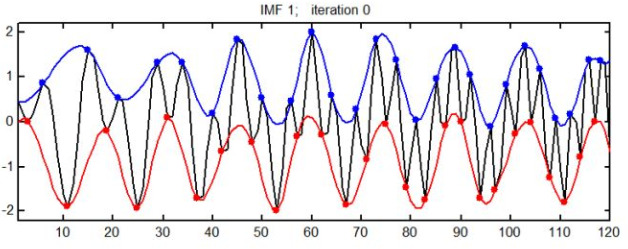
The mean value of the upper and lower envelopes of the IMF.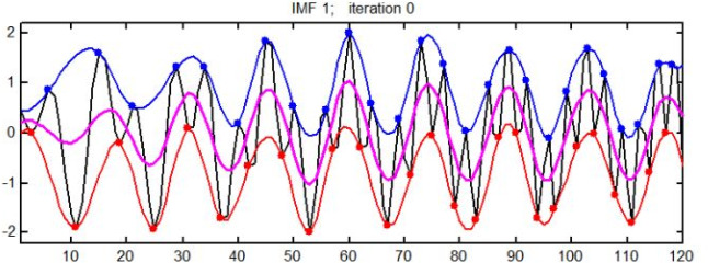

Figure 3.

The difference between the original signal and the envelope average.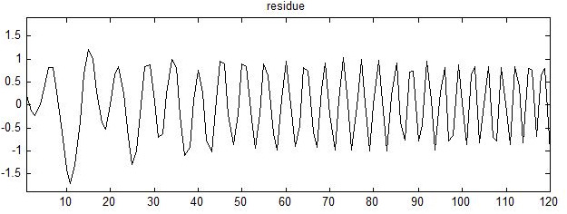

2. Determine whether $f_{1}(t)$ meets the condition requirements of the IMF component. If it is the case, then $f_{1}(t)$ will be the first IMF component of the original signal, if not, then $f_{1}(t)$ will be the new original signal. Repeat step (1) as many times as necessary to satisfy the requirements of the IMF component.

3. When $f_{1}(t)$ is subtracted from the original signal $X(t)$ , $r_{1}(t)$ is obtained. To obtain the second IMF component $f_{2}(t)$ of the original signal and its residue $r_{2}(t)$ , repeat the previous procedure using the new original signal $r_{1}(t)$ .

$\displaystyle\begin{cases}r_{1}(t)=X(t)-f_{1}(t)\\ r_{2}(t)=r_{1}(t)-f_{2}(t)\\ \vdots\\ r_{n}(t)=r_{n-1}(t)-f_{n}(t)\\ \end{cases}$ (3)

4. The EMD decomposition process ends when $r_{n}(t)$ is a monotone function or constant, which corresponds to $n$ IMFs and 1 residue $r_{n}(t)$ . Based on Fig. 4, the original signal $X(t)$ is calculated as follows:

$\displaystyle X(t)=\sum_{i=1}^{n}f_{i}(t)+r_{n}(t)$ (4)

Based on Eq. (4),

$f_{i}(t)$ : $n$ eigenmode functions IMF constituents in descending order.

$r_{n}(t)$ : A potential that represents the signals’ general change tendencies.

Figure 4.

Results of EMD decomposition.

3. LSTM

As a result of gradient disappearance or gradient explosion during transmission, the network level of RNNs needs to be improved in order to prevent the network level from becoming too deep. According to Fig. 5, the system is composed of three doors: input doors, forgetting doors, and output doors. As a result of the information contained in both the input layer and the hidden layer from the previous time, the on/off state of the door is influenced. Using the input door, the unit value $c$ is updated. In order to determine the ratio of the unit value $c$ reserved previously, the forgetting door is used. As a result of the output door, the hidden layer state value $h$ is generated, which is used as an additional input in the subsequent process.

Figure 5.

LSTM memory unit.

The Forget Gate produces the following output when it forgets C ${}_{t-1}$ :

$\displaystyle f_{t}=\sigma(W_{f}\cdot[h_{t-1},x_{t}]+b_{f})$ (5) $\displaystyle i_{t}=\sigma(W_{i}\cdot[h_{t-1},x_{t}]+b_{i})$ (6) $\displaystyle\tilde{c}_{t}=\tanh(W_{c}\cdot[h_{t-1},x_{t}]+b_{c})$ (7) $\displaystyle c_{t}=f_{t}*c_{t-1}+i_{t}*\tilde{c}_{t}$ (8)

The output of the output gate is shown below:

$\displaystyle o_{t}=\sigma(W_{o}\cdot[h_{t-1},x_{t}]+b_{o})$ (9) $\displaystyle h_{t}=o_{t}*\tanh(c_{t})$ (10) $\displaystyle\sigma(x)=\frac{1}{1+e^{-x}}$ (11) $\displaystyle\tanh(x)=\frac{e^{x}-e^{-x}}{e^{x}+e^{-x}}$ (12)

$\sigma$ represents the active function such as Sigmoid or Relu; matrix $W_{f}$ represents the weight coefficient of the forgetting gate; $h_{t-1}$ represents the hidden layer status of the previous time; $x_{t}$ represents the input of the current time; $b_{f}$ represents the bias vector of the forgetting gate; matrix $W_{i}$ represents the weight coefficient of the input door; $b_{i}$ represents the bias vector of the input door; matrix $W_{c}$ is used to update the weight coefficient of the neuron state; $b_{c}$ is used to update the bias vector of the neuron state; matrix $W_{o}$ represents the weight coefficient matrix that is used to update the output; $b_{o}$ represents the bias vector that is used to update the output value; $h_{t}$ represents the output result and returns to the initial state of the hidden layer at the next time.

4. Indicators for forecast evaluation

In order to select a suitable forecasting model, evaluation indicators are indispensable. However, there is no general standard index evaluation system in place at the present time. There are two formulas commonly used to evaluate errors: Average Absolute Error (MAE) and Root Mean Square Error (RMSE). Here are some related formulas:

$\displaystyle\textit{MAE}=\frac{1}{n}\sum_{i=1}^{n}\left|{y_{i}-\hat{y}_{i}}\right|$ (13) $\displaystyle\textit{RMSE}=\sqrt{\frac{1}{n}\sum_{i=1}^{n}(y_{i}-\hat{y}_{i})^% {2}}$ (14)

$y_{i}$ represents the real value and $\hat{y}_{i}$ represents the forecast result value. A smaller indicator value indicates a more accurate model, and a higher forecast accuracy.

5. The forecasting model of EMD-LSTM

LSTM is divided into two steps for predicting short time series. In order to obtain the basic modal components imf with varying scale characteristics, an EMD decomposition is performed on the original time series. In order to predict and analyze each component of the imf, the LSTM neural network is used. The final forecast result is obtained by summarizing the forecast results of each component of the imf. A model combination of EMD-LSTM can be seen in Fig. 6.

5.1 Modeling process

Table 1
Input and output data of modeling

Input	Output
$x_{1},x_{2},x_{3},\ldots,x_{n}$	$x_{n+1}$
$x_{2},x_{3},x_{4},\ldots,x_{n+1}$	$x_{n+2}$
$\ldots$	$\ldots$
$x_{n-N},\ldots,x_{n-1}$	$x_{n}$

Figure 6.

EMD-LSTM prediction model.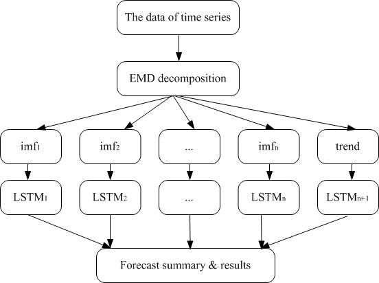

A time series is presented as $S=\{d_{1},d_{2},\ldots,d_{i},\ldots,d_{n}\}$ . In the process of decomposing the EMD, $n$ imf modal components and 1 residue series of trend are generated. As input to the LSTM neural network, $n$ imf components and residue series of trend are used. Finally, the sum of the predicted values for each component is calculated and the result is the final predicted value. The original series $X$ is translated into a series of inputs and outputs before the time series is predicted. There are $n-N$ training modes generated when the length of the original time series is $n$ and the number of input levels is $N$ . Data inputs and outputs are shown in Table 1.

After the input and output data have been divided, they are further divided into training sets, test sets, and validation sets. To train the forecasting model of LSTMLSTM, training sets and test sets are used, while validation sets are used to verify the model’s forecasting capabilities. In general, training sets, test sets, and validation sets are divided into 80% and 20%, respectively.

5.2 Process for training the LSTM network

Time series prediction with LSTM is also one of the keys to the training of LSTM networks, as well as processing of input data, including modal decomposition with EMD and data normalization, while training is primarily targeted at the hidden layer of the network. From the IMF, time series are entered as $S_{\textit{imf}}=\{s_{1},s_{2},\ldots,s_{n}\}$ , which are separated into a training set ( $S_{\textit{train}}=\{s_{1},s_{2},\ldots,s_{m}\}$ ) and a test set ( $S_{\textit{test}}=\{s_{m+1},s_{m+2},\ldots,s_{n}\}$ ). Afterwards, the training set elements are normalized, and the processed training set is $S_{\textit{train}}^{\prime}=\{s_{1}^{\prime},s_{2}^{\prime},\ldots,s_{m}^{% \prime}\}$ . The normalization is performed using the minmax_scale method $X=\frac{X-X.\min}{X.\max-X.\min}*(\max-\min)+\min$ . The data should be segmented in order to meet the input requirements of the hidden level. In the case of a segmented window length of $L$ , the input to the segmented model would be as follows:

$\displaystyle X=\{X_{1},X_{2},\ldots,X_{L}\}$ $\displaystyle X_{t}=\{f_{t}^{\prime},f_{t+1}^{\prime},\ldots,f_{m-L+t-1}^{% \prime}\}$ $\displaystyle 1\leqslant t\leqslant L;\,t,L\in N$

In this case, the output is as follows:

$\displaystyle Y=\{Y_{1},Y_{2},\ldots,Y_{L}\}$ $\displaystyle Y_{t}=\{f_{t+1}^{\prime},f_{t+2}^{\prime},\ldots,f_{m-L+t}^{% \prime}\}$

$X$ ’s input to the hidden layer (including $L$ LSTM units) and $X$ ’s output through the hidden layer can be expressed as

$\displaystyle H=\{H_{1},H_{2},\ldots,H_{L}\}$ $\displaystyle H_{t}=\textit{LSTM}(X_{t},C_{t-1},H_{t-1})$

In the equation, $C_{t-1},H_{t-1}$ represent the state and output of the previous LSTM, respectively. Using the average difference, error calculation is performed, and the training process’ loss function is defined as follows:

$\displaystyle\textit{loss}=\sum_{i=1}^{L(m-L)}{(H_{i}-Y_{i})/L(m-L)}$ (15)

Set optimization targets for loss functions, as well as the initial network random seed (seed), learning rate ( $\eta$ ), and training steps. The hidden layer network is obtained by continuously updating the weight of the network via the Adam optimization algorithm.

6. EMD-LSTM-based forecasting algorithm

Based on the LSTM forecasting algorithm, the EMD-LSTM algorithm was derived. As a result, it modifies the instability of the original LSTM when forecasting data. Consequently, the forecasting process becomes more accurate and adaptable since the data development trend is maintained.

6.1 Eliminate abnormal data

Alternatively, anomaly data may be referred to as isolated data or out-clustered data. There is a significant difference between this data and the normal data in the graph. Due to its presence in the forecast, the establishment of the model is affected, which results in an increase in forecast errors. Multiple methods can be used to eliminate abnormal data. In this article, abnormal data is determined using the following methods:

If $x_{i}\geqslant 3\times\max\{|m_{a}|,|m_{b}|\}$ ,

In this case, $x_{i}$ represents the abnormal data, and its value is replaced by $x_{i}=(x_{i-1}+x_{i+1})/2$ .

Among them

$m_{a}=\textit{mid}(x_{i-3},x_{i-2},x_{i-1})$ , $m_{b}=\textit{mid}(x_{i+1},x_{i+2},x_{i+3})$ , mid() represents a median function.

6.2 The setting of model parameters

When entering data for the LSTM network for training, the nodes and hidden nodes should be designed carefully in order to achieve better prediction of time series data. Repeated experiments, empirical formulas, growth methods, deletion methods, and other methods can be used to determine the number of neural units in the hidden layer of an LSTM network. To determine the roughness of the hidden layer, this chapter combines the growth method, the reduction method, and the empirical formula method. After comparing the accuracy of the results with anti-growth and deletion methods, The number of hidden level nodes are calculated based on the number of nodes with the highest accuracy. In this thesis, the following empirical formula has been adopted:

$\displaystyle n_{1}=\sqrt{n+m}+a$

$n$ represents the number of input layer units. $m$ represents the number of output nodes, $a\in$ [1,10]. An empirical method is used to determine the range of neurons. Following this, the model is trained to increase or decrease the number of neurons, and appropriate neurons are screened based on the error values. Adam can be estimated using adaptation momentum as an optimization algorithm. This algorithm calculates the adaptive learning rate for a wide range of parameters and consumes fewer storage resources

6.3 EMD-LSTM forecasting algorithm

The LSTM training forecast algorithm consists of the steps listed in Algorithm 1.

Algorhtim 1. LSTM training forecast algorithm

Input: The series are

S_{\textit{imf}}

after the decomposition of EMD. Series length is divided into

m

. EMD is decomposed into imf, whose number is

n

. The window of division is

L

, seed, and steps. The learning rate is

\eta

. Output: Series of forecasted outputs and errors associated with the model BEGIN 1. Obtain

S_{\textit{tarin}}

S_{\textit{test}}

from

S_{\textit{imf}}

m

S_{\textit{train}}^{\prime}=\text{minmax{\_}scale}(S_{\textit{tarin}})

3. Obtain

X

Y

from

S_{\textit{train}}^{\prime}

L

4. Initialize the LSTM using the seed 5. Create LSTM 6. For each step in 1: steps 7.

H=\textit{LSTM}(X)

\textit{loss}=\sum_{i=1}^{L(m-L)}{(H_{i}-Y_{i})}/L(m-L)

9. Update LSTM by Adam with loss and

\eta

10. Obtain LSTM

{}^{\ast}

11. For each i in range(m:n) 12.

Y_{m}^{*}

=\text{LSTM}^{*}(X_{m})

13. Append

Y_{m}^{*}

Y^{*}

14.

Y=\text{de{\_}minmax{\_}scale}\left(\sum_{i=1}^{n+1}Y^{*}\right)

15. Return error_measure(Y, Y

{}_{m}

) END

7. Experimental results and analysis

To evaluate the effectiveness and superiority of the EMD-LSTM model, this experiment was verified with a real dataset, which addresses the following two questions: (1) Validity. Time series data are predicted using the EMD-LSTM algorithm and compared with the original time series data. In the case of a small error, the validity can be reflected. (2) Advantage. EMD-LSTM data forecasts are compared with forecasts obtained from other models. In this way, forecasting accuracy will be improved, which will result in a competitive advantage.

7.1 Experimental data

In this thesis, Eamonn Keogh provides the data through his classic time series data website, which is available at http://www.cs.ucr.edu/∼eamonn/ and maintained by Eamonn Keogh. As the experimental object, we select the Synthetic Control series data. These data are derived from real production control, which is divided into two types: test samples and training samples. In both the test and training samples, there are 300 time series, which are divided into six categories, each with 50 samples, resulting in a total of 60 points per sample. Class 1 with Normal characteristics was selected and the test and training samples were combined into 6,000 data points, 500 consecutive data points were randomly selected and split into 80% of training samples and 20% of test samples. Data from Class 2 with cyclic characteristics were selected, and the test sample and the training sample combined to create 6,000 data points. A total of 100 consecutive data points were randomly selected for the experiment and divided into 80% of the training sample and 20% of the test sample. Different data sets can be used to test the effectiveness of the algorithm.

7.2 Experimental setting

Using SVM and LSTM forecasting algorithms and the EMD-LSTM algorithm model proposed in this chapter, a comparative experiment was conducted to verify the effectiveness and feasibility of the EMD-LSTM algorithm model. Synthetic Control series data were utilized as experimental objects to test the proposed method’s forecasting capability.

7.3 Comparison of experiments

We designed two scenarios for the prediction and comparison to test the sophistication of the EMD-LSTM algorithm proposed in this thesis: Program I: EMD-LSTM forecasting for two types of raw data; Program II: LSTM and SVM are employed to predict and compare for both types of data.

Figure 7.

EMD decomposition of Normal data.

Figure 8.

EMD decomposition of Cyclic data.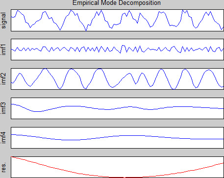

The algorithm is running in the following environment: Intel i7-8565U@1.8GHz Quad-core CPU; 16 G internal storage; 1 TB hard drive for storage capacity of the hard drive; Microsoft Windows Operating System; MATLAB 7.1; python 3.5; tensorflow 1.2 and Keras.

7.3.1 Program I

As a result of the abnormal processing, the two types of data are decomposed by EMD. EMD decomposes the first data set (Normal) into 10 components. The original time series signals are each shown in Fig. 7. An analysis of the inherent mode function (imf1, imf2, …, imf8) shows that the volatility of the function is gradually decreasing, while the stationarity is gradually increasing, and the res represents the trend line. EMD generates six components from the second (cyclical) data. The original time series signals are shown in Fig. 8. The inherent mode function (imf1, imf2, …, imf8) decomposed by EMD shows that its volatility is gradually decreasing and its stationarity is gradually increasing, with res representing the trend line. According to the analysis, the data characterized by Normal have more imf than the inherent modal functions decomposed by Cyclic.

Figure 9.

Predicted Normal type data using EMD-LSTM.

Figure 10.

Cyclic type data predicted by EMD-LSTM

During the experiments, the model sets the initial input to 500, the density to 12, the output to 1, the weight and bias to [ $-$ 1, 1] for each data, and the number of iterations to 100. Each imf is predicted by using the average division error (RMSE) as a loss function, which is accumulated after the prediction is made. According to Fig. 9, the forecast results are shown as above.

In the experiment, the model sets the initial inputs to 100, Dense to 6, output to 1, the initial weight and bias to [ $-$ 1, 1] for each data set, and the number of iterations to 100. Each imf is predicted using the average division error (RMSE) and accumulated after it is predicted. As can be seen in Fig. 10, the forecast results are as above.

An EMD decomposition of the short time series yields the IMF components and trend items of the intrinsic mode function. As a result of the decomposed time series, the volatility and complexity of the short series are eliminated. Next, we use the LSTM to predict and sum up the components of the IMF and trend items in order to obtain the prediction results for the time series. According to Figs 10 and 11, the EMD-LST model algorithms show adaptability and reliability for prediction, regardless of whether the data are normal-type data (representing irregular data) or cyclic-type data (representing periodic data).

7.3.2 Program II

Table 2
Prediction error of Normal data

	SVM	LSTM	EMD-LSTM
MAE	0.8295	0.8291	0.7094
RMSE	0.0972	0.0973	0.0861

Table 3

Prediction error of Cyclic data

	SVM	LSTM	EMD-LSTM
MAE	1.1831	0.5807	0.5271
RMSE	1.399	0.6867	0.5941

Figure 11.

Comparison of three models for predicting data of the Normal type.

Figure 12.

Comparison of three models for predicting data of the cyclic type.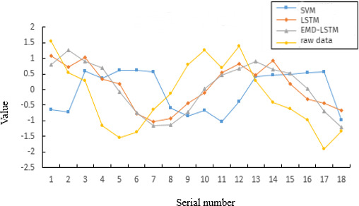

In order to further validate the superiority of the EMD-LSTM model presented in this section, a comparative study is conducted to compare the forecasts of the LTEM, LSTM, and EDM-LSTM models in this theme. The same data is selected as in Program I. In this case, the kernel function of SVM is RBF as the core, and the regularization parameter C and the kernel function parameter gamma are set to 10 and 2, respectively. Program I provides instructions for setting the LSTM and EMD-LSTM parameters.

Figures 11 and 12 illustrate a comparison between forecast data and actual data for each model, along with the corresponding evaluation indicators in Tables 2 and 3. The EMD-LSTM forecasts perform well for both normal and cyclical forecasts. In the case of Cyclic data forecasting, SVM and LSTM are acceptable, but in the case of Normal data forecasting, they are not satisfactory. It can be concluded that the prediction accuracy has improved when compared with other models using the EMD-LSTM algorithm, which is a testament to its superiority.

8. Conclusion

This paper proposes a time series forecasting algorithm based on the EMD-LSTM model. First, anomalous data is eliminated, and then EMD is used to perform modal decomposition. By decomposing the data, the influence of random nature is eliminated, thus improving the forecasting accuracy of LSTM on short time series. Based on experimental validation and comparison, it has been determined that an EMD-LSTM algorithm demonstrated good adaptability and prediction accuracy for a variety of range series, and the use of this approach in scenarios is more widespread.

Footnotes

Acknowledgments

It is supported by the State Key Laboratory of Tibetan Intelligent Information Processing and Application/Tibetan Information Processing and Machine Translation Key Laboratory of Qinghai Province (2020Z003), Fuzhou Polytechnic (FZYRCQD201901), and Fuzhou Polytechnic’s Certification Training Program (LX-2019-HX-005).

References

Zhang

Jia

. Production performance forecasting method based on multivariate time series and vector autoregressive machine learning model for waterflooding reservoirs. Petroleum Exploration and Development. 2021; 48(1): 175-184.

Peng

Wang

, et al. Application of Seasonal Auto-regressive Integrated Moving Average Model in Forecasting the Incidence of Hand-foot-mouth Disease in Wuhan, China. Current Medical Sciences. 2017; 37(6): 842-848.

Liu

Jia

. Research on the application of the segmentation based on key points in the power consumption of wireless sensor. Journal of Applied Science and Engineering. 2016; 19(1): 109-112.

Gou

Liu

Wang

. Radar group target recognition based on HRRPs and weighted mean shift clustering. Journal of Systems Engineering and Electronics. 2020; 31(6): 1152-1159.

Wang

Shen

, et al. Prediction of chaotic time series based on Nyström Cauchy kernel conjugate gradient algorithm. Acta Physica Sinica. 2022; 71(10): 422-431.

Huang

Shen

Long

, et al. The empirical mode decomposition and the Hilbert spectrum for non-linear and non-stationary time series analysis. Proceedings of the Royal Society A – Mathematical Physical and Engineering Sciences. 1998; 454(1971): 903-995.

Miao

Han

Yao

, et al. Application of LSTM for short term fog forecasting based on meteorological elements. Neurocomputing. 2020; 408: 285-291.

Yousuf

Khan

Khursheed

. Remaining useful life (RUL) regression using Long-Short Term Memory (LSTM) networks. Microelectronics Reliability. 2022; 139: 114772.

Men

Ilk

Tang

, et al. Multi-disease prediction using LSTM recurrent neural networks. Expert Systems with Applications. 2021; 177: 114905.

10.

Cortez

Carrera

Kim

, et al. An architecture for emergency event prediction using LSTM recurrent neural networks. Expert Systems with Applications. 2018; 97: 315-324.

11.

Hochreiter

Schmidhuber

. Long short-term memory. Neural Computation. 1997; 9(8): 1735-1780.

12.

Yang

Chao

Nie

, et al. Construction method of hybrid quantum long-short term memory neural network for image classification. Acta Physica Sinica. 2023; 72(5): 474-487.

13.

Qin

Huang

, et al. A novel LSTM-autoencoder and enhanced transformer-based detection method for shield machine cutterhead clogging. Science China Technological Sciences. 2023; 66(2): 512-527.

14.

Wei

Zhang

Yang

, et al. Machine learning for pore-water pressure time-series prediction: Application of recurrent neural networks. Geoscience Frontiers. 2021; 12(1): 453-467.

15.

Bai

. Emergency Detection Method in Social Media Based on CNN-RNN. Journal of the China Railway Society. 2021; 43(8): 97-105.

16.

Zhao

. A multi-attention RNN-based relation linking approach for question answering over knowledge base. Journal of Southeast University (English Edition). 2020; 36(4): 385-392.

Research on the prediction of short time series based on EMD-LSTM

Abstract

Keywords

1. Introduction

2. EMD decomposition principle

5.1 Modeling process

Table 1 Input and output data of modeling

6.1 Eliminate abnormal data

6.2 The setting of model parameters

6.3 EMD-LSTM forecasting algorithm

7. Experimental results and analysis

7.1 Experimental data

7.2 Experimental setting

7.3 Comparison of experiments

Table 2 Prediction error of Normal data

Footnotes

Acknowledgments

References

Table 1
Input and output data of modeling

Table 2
Prediction error of Normal data