Integrating inverse data envelopment analysis and neural network to preserve relative efficiency values

Abstract

The present paper is an attempt to integrate inverse Data Envelopment Analysis (DEA) and Artificial Neural Network (ANN) for a large dataset with multiple Decision Making Units (DMUs). The purpose of this study is to determine the best possible values of inputs for a large number of DMUs when their output levels are changed and their efficiency values remain unchanged. When the ANN is used to develop inverse DEA, it is not necessary to solve the inverse DEA model for every single DMU. Therefore, this approach can save the computer’s memory and the CPU time especially for very large scale datasets. To illustrate the ability of the proposed methodology, a set of 600 Iranian bank branches is used.

Keywords

Artificial neural network data envelopment analysis inverse optimization efficiency resource allocation

1 Introduction

There are diverse methods to evaluate efficiency measure in the literature. Methodologically, they are assorted in accordance with two criteria. The first classification distinguishes between parametric and non-parametric approaches. In the parametric approach, specific analytic function with constant parameters is used to describe the boundary of production possibility set. On the contrary, the non-parametric approach makes no stringent assumptions about production possibility set. The second category differentiates between stochastic and deterministic methods. Deterministic approaches do not allow uncertainty in data whereas the stochastic approach regards the stochastic nature of data. The following stochastic approaches can be cited as the commonly used parametric ones:

Stochastic frontier approach (SFA) which was engendered by Aigner et al. [9], thick frontier approach (TFA) of Berger and Humphrey [1] and distribution free approach (DFA) which was developed by [7]. The non-preferable over parametric ones; on account of the fact that they are intuitive and easy to carry out. The common non-parametric methods are Data Envelopment Analysis (DEA) of Charnes et al. [2] and free disposal hull (FDH) which was first formulated by Deprins et al. [11]. Both the deterministic and stochastic DEA models are extended in the literature. FDH as a deterministic method is the DEA relaxed of the convexity assumption. DEA is a leading approach in distinction from other approaches since DEA needs no explicitly assumptions on the specification of the production function and is capable of evaluating efficiency change over time.

DEA is a method for assessing the productive efficiency of a set of homogeneous Decision Making Units (DMUs) enjoying multiple inputs and outputs. The preliminary objective of DEA is to partition the DMUs into two classes: efficient and inefficient ones. It is based on establishing the efficient frontier via a piecewise form that rests on top of the empirical observations. DEA provides a measure of the efficiency score for an inefficient DMU as its distance from the efficient frontier.

Efficiency evaluation of DMUs (involved complex and often unknown relations between inputs and outputs) are measured easily without requiring superfluous assumptions. The first model in DEA was presented in the CCR paper [2] (after Charnes, Cooper and Rhodes). In the CCR model, the efficiency of each DMU is obtained as the maximum of a ratio of weighted outputs to weighted inputs subject to the constraint that the similar ratio for all DMUs is less than or equal to one. Subsequently, Banker et al. [29] proposed a variable returns to scale version of the CCR model which was named the BCC model (after Banker, Charnes and Cooper). To acquaint with other DEA models, the reader is referred to [24, 25].

There has been a widespread tendency in both theoretical developments and applications in DEA literature. In regards to the development of DEA applications, Liu et al. [22] provided a systematic survey of DEA applications. They reported that, on the whole, two-third of DEA studies incorporated applications while the remaining one-third focused on purely-methodological. Their results indicated the five major DEA applications as banking, health care, agriculture and farm, transportation, and education.

Extensive surveys are introduced in regards to the DEA methodologies and its theoretical developments, as the following examples show. Seiford [24] traced the evolution map of DEA from inception to the year 1995 and provided an extensive bibliography of DEA during a 17-year period. Cooper et al. [34] described some of DEA models and noted their properties. So they demonstrated relations between the models and the associated measures of efficiency. Liu et al. [21] studied the DEA literature by applying a citation-based approach. They addressed the most influential DEA paper and the five most active DEA subareas. A sketch of the major methodological developments of DEA covering its 30 years of history is available in [33].

The efficiency of each DMU in DEA is clearly designated by its input and output levels. Therefore, changes in input or output values can induce changes in the relative efficiency values of DMUs. Inverse DEA is discussed to maintain current efficiency value of a given DMU if its internal structure changes. Inverse DEA models are classified into two bundles relying on which parameters are changed and which parameters must be adjusted with the understanding that the efficiency remains unchanged. These two types are the investment analysis problem and the resource allocation problem. The investment analysis problem of DEA is an inverse DEA problem in estimating output levels for the given inputs, under the condition of preserving the efficiency index. In contrast, the resource allocation problem deals with determining possible inputs for the demanded outputs while the efficiency score stays unchanged. For the first time, Wei et al. [28] intimated inverse DEA model to answer the following question: among a group of DMUs, if we increase certain inputs to a particular unit and assume that the DMU maintains its current efficiency level with respect to other units, how much more outputs could the unit produce? Or, if the outputs need to be increased to a certain level and the efficiency of the unit remains unchanged, how much more inputs should be provided to the unit? They assumed that the increase in input and output values to be nonnegative values and proposed a multi-objective linear programming (MOLP) for inefficient DMUs and a linear programming (LP) for weakly efficient DMUs. Subsequently, Yan et al. [19] discussed the inverse DEA problem with preference cone constraint to provide the properties of the inverse DEA problem through a discussion of its related multi-objective and weighted sum single-objective programming problems. Jahanshahloo et al. [16] expanded the method presented by Yan et al. [19] and proposed a method to estimate output levels of a DMU when some or all of its input entities were increased and its current efficiency level was improved. Jahanshahloo et al. [17] showed that the inverse DEA models could be used to estimate inputs for a DMU when some or all outputs and the efficiency level of the DMU were increased or preserved. They also introduced an approach to identify extra inputs when the outputs were estimated using the proposed models by Yan et al. [19] and Jahanshahloo et al. [17]. Hadi-Vencheh and Foroughi [6] amplified the work of Wei et al. [28] by allowing a simultaneous increase of some inputs (outputs) and a decrease of some other inputs (outputs). Moreover, they proposed a MOLP model for both inefficient and weakly efficient DMUs. In addition, they showed that the solution proposed by Wei et al. [28] did not guarantee the efficiency result for input estimation and introduced some solutions to overcome this failure. Lertworasirikul et al. [30] considered the inverse BCC model for a resource allocation problem. Their developed model keeps the relative efficiency values of all DMUs in a new production possibility set composing of all current DMUs and a perturbed DMU with new input and output values. The inverse BCC problem was in the form of a multi-objective nonlinear programming model (MONLP) which was not easy to solve. They proposed a LP model which gives a Pareto-efficient solution to the inverse BCC problem. Jahanshahloo et al. [18] analysed inverse DEA under inter-temporal dependence assumption. They used solutions of a new optimality notion for MOLP, the periodic weak Pareto optimality in inverse DEA. They illustrated that these solutions can be characterized by a simple modification in weighted sum scalarization tool.

Artificial Neural Networks (ANNs) are information processing algorithms that emulate the behavior of neurons in the brain. They can be applied to approximate complex relationships between sets of variables. Therefore, ANNs have extensive applications in many areas such as weather forecast, air traffic control, medical research, economics, and finance. Various approaches have been proposed aiming at contributing to the use of ANN in DEA. The first combination of ANN and DEA to assess performance measurement was introduced by Athanassopoulos and Curram [4]. They demonstrated that both methods offer a useful range of information regarding the assessment of performance. Emrouznejad and Shale [5] combined ANN with DEA to introduce an approach to estimate the efficiency of DMUs in large data sets. The results indicated that the ANN-DEA prediction of the efficiency score appears to be a good estimate for the majority of DMUs. According to Santin et al. [13], ANNs constitute a promising alternative to traditional approaches, econometric models, and non-parametric methods such as DEA in order to fit production functions and measure the efficiency under non-linear contexts. Costa and Markellos [3] proposed an ANN approach to measure performance of public transport services. They analyzed the London underground efficiency with time series data and explained that the ANN approach is superior to traditionally applied techniques since it is both nonparametric and stochastic and offers greater flexibility. Additional related approaches can also be found in references such as [14 , 35]. The related literature vastly shows the applicability of ANN in predicting the DEA results. Moreover, it indicates that DEA and ANN can successfully assist each other. In this study, a combination of resource allocation problem and ANN is employed which serves to estimate the necessary input levels for the production of demanded output levels while the efficiency values of all DMUs remain unchanged. In contrast with inverse DEA models, the proposed method does not need to be reprogrammed. Also, it is simple to be implemented in parallel architectures. This reduces the processing time compared to inverse DEA models with similar results. The rest of the paper unfolds as follows. In Section 2, inverse DEA model and the method of calculation in inverse DEA are described. Section 3 explains the ANN approach which is followed by a back-propagation algorithm. An ANN algorithm for inverse DEA, namely ANN-inverse DEA is introduced in Section 4. Section 5 reports results from the application of ANN-inverse DEA to a really large set of Iranian bank branches. Finally, Section6 deals with the concluding remarks.

2 Preliminaries

Suppose there are n DMUs, {DMU_j : j = 1, …, n} each using m inputs to produce s outputs and also assume x_j = (x_1j, x_2j, …, x_mj) ^T , y_j = (y_1j, y_2j, …, y_sj) ^T to be the input and output vectors for DMU_j, respectively, such that x_j ≥ 0 , x_j ≠ 0 and y_j ≥ 0 , y_j ≠ 0. To evaluate the efficiency of DMU_o using BCC model, we have: $\begin{matrix} θ_{o}^{*} = min θ \\ s . t . \sum_{j = 1}^{n} λ_{j} x_{ij} \leq θ x_{io}, i = 1, \dots, m \\ \sum_{j = 1}^{n} λ_{j} y_{rj} \geq y_{ro}, r = 1, \dots, s \\ \sum_{j = 1}^{n} λ_{j} = 1 \\ λ_{j} \geq 0, j = 1, 2, \dots, n \end{matrix}$ (1)

where λ_j is the intensity variable for DMU_j and $θ_{o}^{*}$ is the efficiency index of DMU_o. If $θ_{o}^{*} = 1$ , then DMU_o is called (at least) weakly efficient.

Following the studies conducted and the trends taken in inverse DEA [6 , 28], Lertworasirikul et al. [30] supposed that DMU_o, among a group of current DMUs with their relative efficiency values of $θ_{1}^{*}, θ_{2}^{*}, \dots, θ_{n}^{*}$ , changes its output levels to y_o + Δy_o ≥ 0, Δy_o ≠ 0.

They specified the minimum Δx_o where x_o + Δx_o ≥ 0 such that DMU_n+1 with new input and output values (x_o + Δx_o , y_o + Δy_o) still has its relative efficiency value of $θ_{o}^{*}$ and all the other DMUs still have their relative efficiency values of $θ_{1}^{*}, θ_{2}^{*}, \dots, θ_{n}^{*}$ . They constructed a new production possibility set composing of n+1 DMUs (DMU_j, j = 1, 2, …, n, and DMU_n+1) which preserved the production frontier. To this end, they proposed the following inverse BCC model: $\begin{matrix} min Δ x_{o} \\ s . t . \sum_{j = 1}^{n} λ_{j} x_{ij} \leq θ_{o}^{*} (x_{io} + Δ x_{io}), i = 1, \dots, m \\ \sum_{j = 1}^{n} λ_{j} y_{rj} \geq (y_{ro} + Δ y_{ro}), r = 1, \dots, s \\ \sum_{j = 1}^{n} λ_{j} = 1 \\ λ_{j} \geq 0, j = 1, 2, \dots, n \end{matrix}$ (2) where $θ_{o}^{*}$ is the relative efficiency value of DMU_o before any changes in its output levels. It is obtained by model (1). They asserted Δx_o from model (2) does not change the relative efficiency values of all DMUs whatsoever.

Moreover, they proved there exists at least an optimal solution to model (2) if and only if y_o + Δy_o ∈ P_out where $\begin{matrix} P_{out} = {y | y \leq Y λ, e^{T} λ = 1, λ \geq 0}, \\ Y = [y_{rj}]_{s \times n}, λ = (λ_{j})_{n \times 1}, λ \in R^{n} . \end{matrix}$

In light of this discussion, they determined a set of non-dominated DMUs based on the output comparisons. As a result, they explained if all the elements of y_o + Δy_o are less than or equal to all the elements of the outputs of at least one DMU in the non-dominated set, then y_o + Δy_o ∈ P_out.

Definition. $(\bar{Δ x_{o}}, \bar{λ})$ is said to be a Pareto optimal solution for model, if there is no other feasible solution (Δx_o, λ) such that $(Δ x_{io} \leq \bar{Δ x_{io}})$ for all i = 1, 2, …, m, with at least one strict inequality, $(Δ x_{io} < \bar{Δ x_{io}}) .$

Via the theory of multi-objective optimization, Δx_o which is obtained by solving the following model, will be a Pareto solution of the inverse BCC model, $\begin{matrix} min w^{T} Δ x_{o} \\ s . t . \sum_{j = 1}^{n} λ_{j} x_{ij} \leq θ_{o}^{*} (x_{io} + Δ x_{io}), i = 1, \dots, m \\ \sum_{j = 1}^{n} λ_{j} y_{rj} \geq (y_{ro} + Δ y_{ro}), r = 1, \dots, s \\ \sum_{j = 1}^{n} λ_{j} = 1 \\ λ_{j} \geq 0, j = 1, 2, \dots, n \end{matrix}$ (3) where w = (w₁, w₂, …, w_m), and w_i : i = 1, 2, …, m is the weight for each unit of input i.

3 Artificial neural network

ANNs can learn from training samples like human brains, and they have the capability to decide based on the data from past training. The structure of generic ANNs consists of layers and neurons (node) as connection weights. Neurons are processing elements which are fully in connection with each other between consecutive layers. Multi-layer Perceptrons (MLP) is one of the most popular and widely used ANN types. MLP includes three different layers:

The input layer simultaneously receives inputs of the ANN; each input needs one node. This layer shifts the data to the linkage layer, so it is not used to perform any calculations. The output layer refers to the estimation of the network and has neurons as outputs of the ANN.

One or more hidden layers with an arbitrary number of computational nodes lie between the input and the output layers. While each data set is given to the ANN, hidden layers manage the internal mapping and let the ANN to learn and generalize the new data by the formerly learned data sets. Therefore, choosing the number of hidden layers and the number of nodes in each hidden layer is important. It is noteworthy that a network with few hidden layers and hidden nodes inhibits identifying the structure of training patterns. On the other hand, owing to extra calculations, the large number of hidden layers and nodes in each hidden layer is associated with longer training time. In most cases, the best structure of hidden layers is determined through a trial and error process. MLP is feed-forward due to the connections between neurons which are in one direction from the input layer to the output layer without any feedback. An example of an MLP is shown in Fig. 1. The illustrated MLP has three input neurons, two outputs and two hidden layers with four neurons in each.

Fig.1

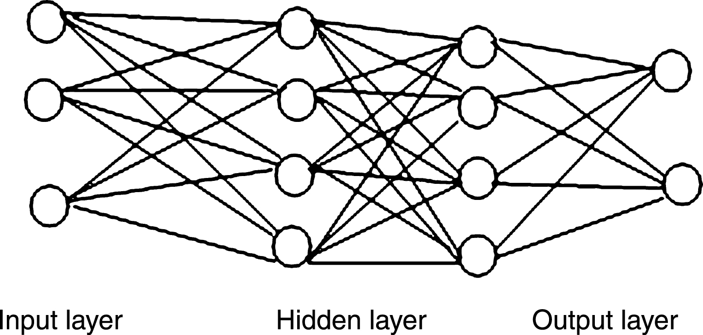
The structure of MLP.

There are two different modes of learning ANNs: supervised and unsupervised. For a supervised learning algorithm, the outputs are known for the given inputs. For an unsupervised learning algorithm, no outputs are specified for a set of inputs. The MLP network is utilized in a supervised manner. Back-Propagation (BP) of Rumelhart et al. [12] is the most popular learning algorithm for a training MLP. Celebi and Bayraktar [10] reminded that the popularity of BP is because of its high level of accuracy and low level of complexity. BP algorithm takes training datum of input patterns and the related set of desired output patterns along with small arbitrary weights.

Following the propagation of inputs in the input layer and directly passing them through the first hidden layer, the weighted inputs are summed up in each node and the result is transferred to an activation function in order to transmit an output from the node. The consequence can be an input to the second hidden layer (if there is any), and so on. Finally, the outcome of the last hidden layer is used as the input for the output layer and the network’s prediction is provided by transforming the sum of weighted inputs into an activation function. In case there is a difference between the desired output and the output produced by the network, the connection weights should be altered and adjusted so as to minimize the Mean Squared Error (MSE) as follows: $E = \frac{\sum_{p = 1}^{P} \sum_{i = 1}^{n_{1}} (y_{i - observed}^{p} - y_{i - prediction}^{p})^{2}}{{Pn}_{1}}$ (4)

Where n₁ is the number of nodes in the output layer and P is the number of learning samples (input-output pairs). This error will be distributed in the backward direction from the output layer through each hidden layer down to the first hidden layer. This leads to the so-called Back-Propagation algorithm.

Fig.2

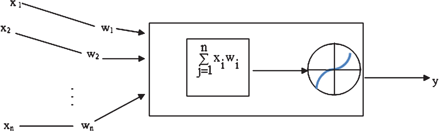
Operation of neuron in BP algorithm.

Figure 2 illustrates a computational neuron of BP algorithm in which x₁, x₂, x₃, …, x_n are inputs of the neuron and w₁, w₂, w₃, …, w_n respectively show their weights. Output of the neuron is then computed as: $y = f (\sum_{i = 1}^{n} x_{i} w_{i})$ (5) where f is the activation function. The activation function is chosen such that it can be non-decreasing and continuously differentiable.

4 The proposed ANN approach for inverse DEA (ANN-inverse DEA)

In this section, ANN-inverse DEA approach will be proposed to develop the inverse BCC model to preserve relative efficiency values of all DMUs. At first, the researchers design a network to estimate the efficiency scores of DMUs. To do so, inputs and outputs in the corresponding DEA model are defined as variables in the input layer and the DEA efficiency score is used as the only variable in the output layer.

Then changes in the output levels of several DMUs, e.g. DMU_{j_k} : k = 1, 2, …, K, are taken into consideration. The purpose is to propose ANN to estimate the input levels of these DMUs so that the relative efficiency values of all DMUs remain unchanged with no need to solve the resource allocation problem for every single DMU.

The analysis of the proposed network is managed in the following steps:

Step 1: configuring the architecture of the ANN-inverse DEA

In the ANN modeling, the researcher should decide on selecting the architecture components such as the inputs and outputs of the network, the number of hidden layers and that of neurons in each hidden layer, the initial values of weights, and the activation function. In the integrated approach, the architecture components include the following:

Inputs of the network: the original input and output values, the new outputs, and the efficiency value of each DMU are utilized as inputs of the network.

Outputs of the network: the new input values that should be predicted by the resource allocation problem, namely Δx_o are selected as the outputs of the network.

Number of hidden layers and the number of neurons in each hidden layer: It is noteworthy that the number of hidden layers and the number of neurons in each hidden layer are decided by trial and error.

Weights: Before training begins, the weights are set to small random values, close to zero.

Activation function in output layer: in the present study, linear activation function is used in the output layer.

Activation function in the hidden layer: sigmoid function is used in the hidden layer as follows: $f (x) = \frac{1}{1 + e^{- x}}$ (6)

where x refers to $\sum_{i = 1}^{n} x_{i} w_{i}$

Step 2: partition data into two data sets

The data set is partitioned into two subsets:

Training set: The training pattern is used to fit the ANN-inverse DEA parameters and to find the optimal weights

Testing set: The testing data is used in order to validate the learned ANN-inverse DEA system.

Step 3: normalizing the data

Since sigmoid function will generate output values in [0,1] and due to the different ranges of inputs, normalization of all data in an acceptable range will help speed up the learning phase and will lead to smooth imperfection of the network. Via the following function, all data are normalized in [0,1]. $p_{n} = \frac{p_{i} - p_{min}}{p_{max} - p_{min}}$ (7) where: p_i= the original value of the ith component of input vector

p_n= the normalized value of p_i

p_min= minimum value among all the ith component values

p_max= maximum value among all the ith component values

Step 4: training ANN-inverse DEA by training set.

The aim of the training phase is to alter the values of the weighted connections to calculate more precise outputs. Thus the sequence of iterations, each called an epoch, is followed in the training process. Each of these epochs is completed when data set of inputs and desired outputs are presented to the network and the weights are adjusted to reduce the MSE. The errors between the network output values and the desired outputs are propagated back through the network so that they are imputed to the weight connections. BP minimizes the MSE via the gradient (steepest) descent method by updating the network weights according to: $w_{new} = w_{old} - η \nabla E$ (8)

Where

$\nabla E = (\frac{\partial E}{\partial w_{1}}, \frac{\partial E}{\partial w_{2}}, \dots, \frac{\partial E}{\partial w_{n}})$ and η is the learning rate.

The learning rate represents the rate of improvement in the training phase and is user-designated (between 0 and 1). If the learning rate is too large, it results in oscillatory learning or converges to a local minimum. On the contrary, if the learning rate is too small, it leads to a long training time but can more closely represent relationships between input and output variables.

The training process is considered complete if any of the following conditions known as stopping criteria is satisfied.

A fixed number of epochs are repeated.

The MSE falls below a threshold value.

Step 5: Testing ANN-inverse DEA approach by testing set.

The generalization capability of the ANN-inverse DEA is confirmed by evaluating its performance on an independent set of data (testing set).

Step 6: Estimating the predicted outputs using the generated ANN-inverse DEA process.

At this stage, the necessary inputs in regard with the resource allocation problem are estimated, which keep the efficiency scores of all.

5 The case study

In this section, the results from the application of the integrated approach are reported. A large set of 600 bank branches in Iran were gathered. The problem of identification of the banking inputs and outputs is a controversy in the literature [15, 23, 26, 27]. There is not consistency concerning the role of input and output selections due to different research objectives in banking. For instance, Isik and Hassan [20] involved labor, capital and loanable funds as input measures and short-term loans, long-term loans, off-balance-sheet items and other earning assets as output measures. Chang et al. [32] used two inputs, physical capital and labor and two outputs, total loans and other earning assets. Halkos and Salamouris [15] used five financial ratios as outputs with no input measures. They argued that all banks manage in the same market; consequently, the inputs are identical for all banks. Weill [26] selected Personnel expenses, other noninterest expenses and interest paid as inputs and loans and investment assets as outputs. Wang et al. [23] defined fixed assets and labors as inputs and Interest income, non-interest income and bad loans as outputs. In addition, deposits are considered as Intermediate measures. Lastly, in order to consider the most relevant and acceptable items of banking system, which are commonly used for measuring efficiency in the literature, this study regards the following categories of inputs:

Input1 (personnel) includes personnel expenses. Input2 (Payable interest) refers to interest expense and revenue. Input3 (Deferred receivables) concerns to Instalments of deferred receivables and deferred payment credits.

And the following categories of outputs are considered:

Output1 (Facilities) consists of term loans, cash credit, overdraft, letters of credit, and bank guarantees. Output2 (The total sum of four main deposits) refers to demand deposits, short-term investment deposits, long-term investment deposits, and foreign currency deposits. Output3 (Received interest) represents earning assets into investment and interest income. outpu4 (Fee received) includes fee income and fee- based services. output5 (Other deposits) refers to other earning asset, Commercial deposits and Retail deposits. It is worth stressing that all inputs and outputs are measured in terms of Iranian million Rials.

Tables 1 and 2 relate a summary of the statistical properties for inputs and outputs.

Table 1
Summery statistic of input values

Inputs

Personnel Payable interest Deferred receivables

Max 88.15 513160 1064400

Min 2.26 41.603 1.4824

Average 14.28 8395.6 18453

Standard deviation 10.17 25090 76816

Median 11.59 3535.7 2500.2

Inputs
Max	88.15	513160	1064400
Min	2.26	41.603	1.4824
Average	14.28	8395.6	18453
Standard deviation	10.17	25090	76816
Median	11.59	3535.7	2500.2

Table 2

Summery statistic of output values

Outputs
	Facilities	Sum of deposits	Received interest	Fee received	Other deposits
Max	8818600	10857000	875880	394980	5216200
Min	2087.4	9327.6	0.569	0.056	0.21
Average	124830	124790	10444	1105.8	10706
Standard deviation	454580	464040	45925	16153	212980
Median	47275	62697	3197.2	163.39	193.740

The first and the second rows in Tables 1 and 2 are the parameter values associated with the normalization equation Equation (7). After normalizing the data, we designed an ANN to measure the efficiency scores of 600 bank branches. For more details of this ANN, readers are referred to [4 , 35]. The efficiency results for the randomly-selected sample of 200 bank branches are listed in Table 3.

Table 3

Bank branch’s efficiency scores

Branch	Efficiency	Branch	Efficiency	Branch	Efficiency	Branch	Efficiency	Branch	Efficiency	Branch	Efficiency
4	0.3224	117	0.4079	217	0.7740	306	0.7562	405	0.6660	511	0.2618
7	0.3111	119	0.5096	218	0.3358	309	0.9698	409	0.3403	513	0.4502
11	0.2901	121	0.9750	221	0.3854	311	0.3508	412	0.4477	517	0.3494
14	0.2575	124	0.9604	223	0.5110	313	0.3117	415	0.9263	521	0.5415
17	0.3011	127	0.3186	226	0.3713	316	0.2946	418	0.9830	523	0.4181
20	0.4257	135	0.2705	228	0.4008	320	0.5234	420	0.4412	526	0.4330
23	0.4382	139	0.6509	232	0.6377	322	0.4597	422	0.6142	529	0.3462
29	0.5137	140	0.3427	234	0.3582	327	0.9616	425	0.5067	532	0.4289
33	0.5906	141	0.8301	236	0.8650	331	0.5297	429	0.4427	534	0.3573
39	0.4606	144	1.1103	239	0.4893	334	0.3943	432	0.6662	538	0.9885
42	0.5561	146	0.8951	242	0.3683	336	0.4775	435	0.3840	541	0.4543
43	0.2997	151	0.6651	243	0.3978	338	0.3362	438	0.2831	543	0.3385
46	0.6308	153	0.2615	246	0.9705	342	0.2706	440	0.6727	546	0.5987
49	0.3675	154	0.5358	249	0.3367	347	0.6341	444	0.2112	547	0.3162
53	0.4791	157	0.4839	251	0.3561	350	0.9310	446	0.3356	554	0.2925
57	0.5455	159	0.5519	253	0.3236	353	0.3195	449	0.3501	556	0.4805
60	0.2385	161	0.8645	256	0.6808	356	0.4185	450	0.2705	558	0.5577
64	0.3152	162	1.0000	258	0.5546	360	0.2514	455	0.4297	561	0.4439
66	0.3239	165	0.4528	262	0.6909	362	0.4657	458	0.3011	564	0.7220
68	0.3130	167	0.7075	264	0.2016	365	0.3987	461	0.4557	568	0.4129
72	0.2901	171	0.4723	268	0.7278	368	0.4024	464	0.2777	572	1. 0600
73	0.4853	174	0.8754	272	0.3632	371	1.0000	468	0.7498	575	0.5127
78	0.3186	178	0.2943	273	0.9304	372	0.2495	473	0.3100	577	0.5776
83	0.6195	181	0.4516	277	0.9915	376	0.2492	476	0.7278	579	0.4035
88	0.6528	184	1.0000	279	0.3013	379	0.4831	477	0.6604	582	0.4437
90	0.3926	186	0.4538	281	0.3602	383	0.9575	483	0.2754	586	0.2932
93	0.7959	191	0.5004	284	0.5023	386	0.3558	485	0.8932	589	0.3601
96	0.3776	195	0.4326	287	0.3804	387	0.2661	488	0.6062	592	0.4011
99	0.4589	198	0.4563	290	0.4503	389	0.4603	491	0.3659	595	0.9462
103	0.4742	201	1.1020	293	0.2661	392	0.2494	494	0.7589	598	0.2700
106	0.9917	204	0.8110	296	1.0245	394	0.3899	497	0.2317
110	0.5900	205	0.7892	297	0.5902	397	0.4400	500	0.2114
112	0.3741	210	0.5065	300	0.3130	399	0.4201	502	0.2535
115	0.3485	215	0.3126	303	0.4946	402	0.2211	509	0.4537

Now suppose the outputs of 237 branches are changed so that positive and negative changes are taken into account at the same time. The stochastic properties of new outputs are summarized in Table 4. It has been straightforwardly confirmed that new outputs are in P_out. Hence model (2) can estimate the necessary inputs while the efficiency values of all branches remain unchanged.

Table 4

Summery statistic of new output values

Outputs
	Facilities	Sum of deposits	Received interest	Fee received	Other deposits
Max	112000	184000	20809	4307.4	7940
Min	9092.2	61840	17.1674	2.245	0.5
Average	87626	92056	2928.6	222.92	479.93
Standard deviation	10302	12831	2348.4	328.01	1005
Median	88295	91167	2450.9	160.7347	143.7001

In this research, the aim has been to employ the ANN-inverse DEA to estimate inputs for 237 banks such that the efficiency scores of 600 banks remain unchanged. To this end, the illustrated neural network from the previous section will be used. At first, the original input and output values of 237 banks, their efficiency scores, and their new outputs as inputs of the ANN-inverse DEA are normalized. Afterward, these branches are partitioned into two parts, the training set and the validation set. 75% of the branches are used as the training set which determine the optimal network parameters, and the remaining 25% are used as the validation set which serve to evaluate the network generalization capability. The reason for selecting a high percentage of data for training is that the network could recognize the patterns governing the inputs and outputs and accommodate to different conditions in a better way. Let w = (1, 1, 1) be the input weights in model (3) for the branches in the training set. The researchers trained the ANN-inverse DEA to approximate input values in model (3). After following the pre-specified epochs or the satisfying condition on the MSE, the network learns non-linear mapping between the inputs and the outputs of the system. Subsequent to the network training, other branches are considered for testing the network. Parameters of the estimated neural network in the ANN-inverse DEA approach are presented in Table 5. Statistical results of input estimation by the ANN-inverse DEA are given in Table 6.

Table 5

Estimated neural network parameters

Concept	Result
Number of neurons input-hidden-hidden-output	14-20-15-3
Activation function hidden/output hidden/output	Sigmoid/linear
Epochs(max)	2000
Mean square error	0.01
Learning rate	0.6

Table 6

Summery statistic of estimated input values

Inputs
	Personnel	Payable interest	Deferred receivables
Max	38.9427	17337	61330
Min	5.3449	586.57	23.924
Average	17.8968	3550.9	4356.2
Standard deviation	6.7640	2128.3	7945.5
Median	17.0146	3055.4	1473

To verify the credibility of the obtained results, the efficiency values of 600 bank branches (by applying new inputs and outputs) are gauged as before by the ANN. Ultimately, comparison of efficiencies by the original inputs and outputs and the new ones are analyzed through the following policies:

Table 7 reports the new efficiency values for a sample of 200 randomly selected bank branches given in Table 3.

From Tables 3 and 7, it can be seen that efficiency scores for certain bank branches are more than 1. This is not voidable in the DEA context. It is not, however, a surprising result for DEA-ANN, since ANN with statistical properties generate a stochastic frontier according to efficient DMUs (Desheng et al., [35]).

In what follows, Fig. 3 depicts a comparison of the efficiency scores for the remaining branches before and after changes in 237 branches (note that 200 random branches in Tables 3 and 7 are not considered). Figure 3a regards bank branches No. 1-299, and Fig. 3b regards bank branches No. 300-600.

Figure 4 shows histogram of efficiency to the 600 evaluated bank branches according to the original inputs and outputs and new ones.

Table 7

Bank branch’s efficiency scores with new inputs and outputs

Branch	Efficiency	Branch	Efficiency	Branch	Efficiency	Branch	Efficiency	Branch	Efficiency	Branch	Efficiency
4	0.3246	117	0.4166	217	0.7717	306	0.7553	405	0.6665	511	0.2635
7	0.3106	119	0.5128	218	0.3328	309	0.9951	409	0.3394	513	0.4517
11	0.2912	121	1.0000	221	0.3847	311	0.3491	412	0.4441	517	0.3501
14	0.2554	124	0.9804	223	0.5123	313	0.3123	415	0.9220	521	0.5430
17	0.2985	127	0.3205	226	0.3741	316	0.2933	418	0.9628	523	0.4156
20	0.4286	135	0.2691	228	0.3974	320	0.5251	420	0.4397	526	0.4337
23	0.4400	139	0.6512	232	0.6335	322	0.4604	422	0.6139	529	0.3471
29	0.5121	140	0.3456	234	0.3574	327	0.9714	425	0.5049	532	0.4300
33	0.5921	141	0.8322	236	0.8664	331	0.5261	429	0.4450	534	0.3542
39	0.4596	144	1.1080	239	0.4900	334	0.3928	432	0.6648	538	0.9874
42	0.5537	146	0.9011	242	0.3665	336	0.4745	435	0.3858	541	0.4565
43	0.3000	151	0.6679	243	0.3943	338	0.3357	438	0.2825	543	0.3359
46	0.6300	153	0.2622	246	0.9681	342	0.2723	440	0.6705	546	0.5963
49	0.3664	154	0.5323	249	0.3377	347	0.6363	444	0.2101	547	0.3152
53	0.4802	157	0.4808	251	0.3536	350	0.9479	446	0.3325	554	0.2920
57	0.5437	159	0.5502	253	0.3242	353	0.3173	449	0.3525	556	0.4823
60	0.2362	161	0.8661	256	0.6821	356	0.4171	450	0.2683	558	0.5542
64	0.3144	162	0.9822	258	0.5514	360	0.2535	455	0.4308	561	0.4443
66	0.3155	165	0.4508	262	0.6932	362	0.4645	458	0.3027	564	0.7232
68	0.3146	167	0.7119	264	0.1984	365	0.3936	461	0.4583	568	0.4136
72	0.2913	171	0.4738	268	0.7258	368	0.4016	464	0.2756	572	1.1606
73	0.4836	174	0.8593	272	0.3659	371	1.0113	468	0.7502	575	0.5149
78	0.3230	178	0.2952	273	0.9282	372	0.2505	473	0.3100	577	0.5759
83	0.6208	181	0.4535	277	0.9817	376	0.2506	476	0.7263	579	0.4018
88	0.6524	184	0.9873	279	0.2983	379	0.4825	477	0.6593	582	0.4452
90	0.3941	186	0.4558	281	0.3587	383	0.9326	483	0.2737	586	0.2915
93	0.7930	191	0.5017	284	0.5006	386	0.3532	485	0.9045	589	0.3618
96	0.3745	195	0.4318	287	0.3833	387	0.2639	488	0.6035	592	0.3967
99	0.4605	198	0.4565	290	0.4495	389	0.4625	491	0.3678	595	0.9543
103	0.4725	201	1.0063	293	0.2656	392	0.2511	494	0.7581	598	0.2700
106	0.9814	204	0.8135	296	1.0608	394	0.3905	497	0.2321
110	0.5925	205	0.7871	297	0.5935	397	0.4412	500	0.2106
112	0.3719	210	0.5081	300	0.3128	399	0.4191	502	0.2511
115	0.3462	215	0.3134	303	0.4933	402	0.2234	509	0.4524

Fig.3

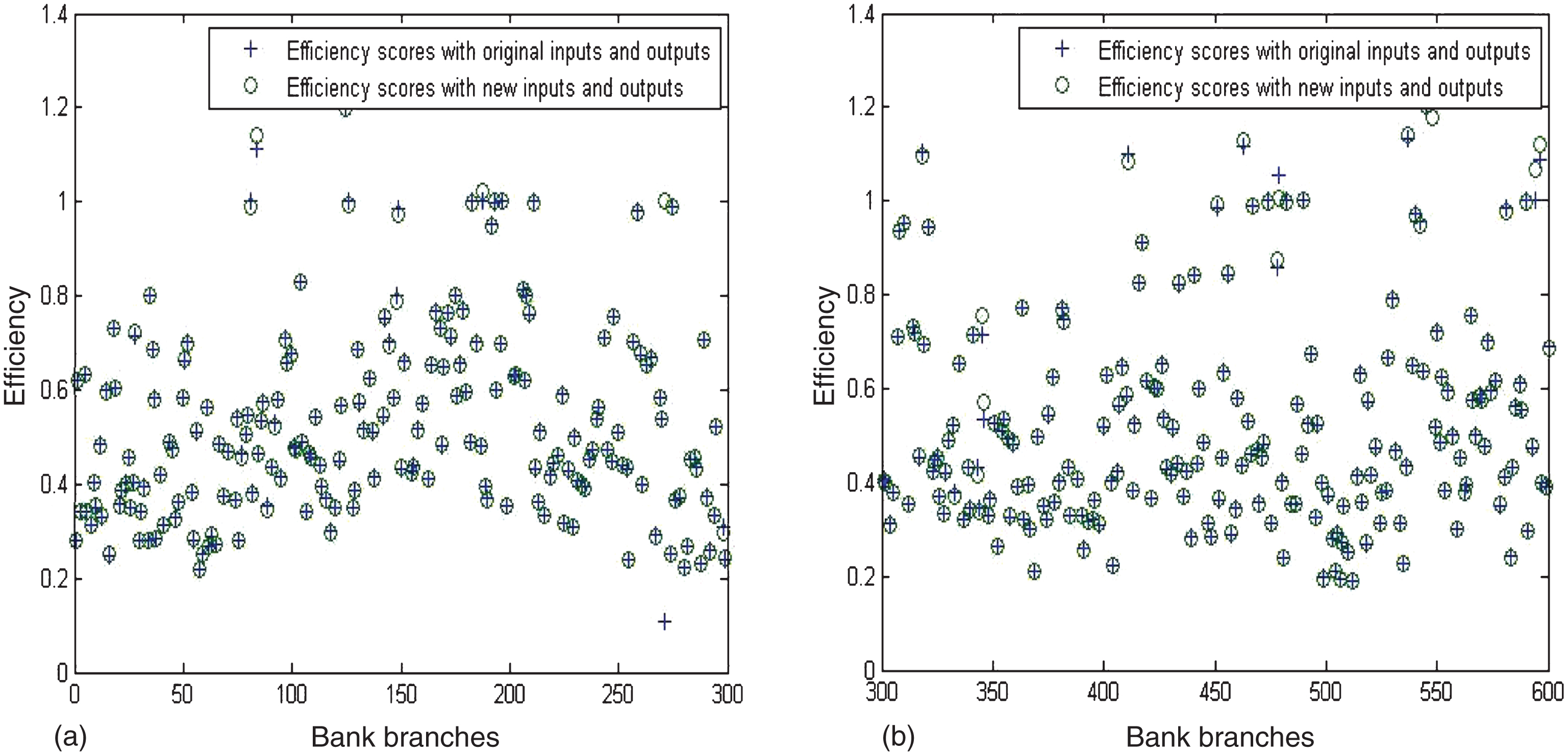
Efficiency scores of bank branches (a) bank branches No. 1-299, (b) bank branches No. 300-600.

Fig.4

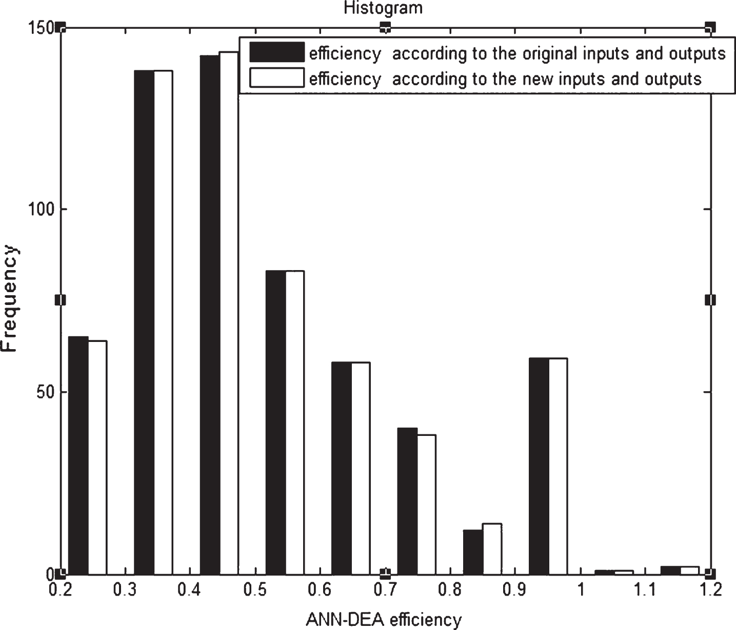
Histogram of efficiency to the 600 evaluated bank branches according to the original inputs and outputs and newones.

As is evident by Fig. 4, the histogram of efficiency measures following original inputs and outputs is drastically similar to the histogram of efficiency results according to the new inputs and outputs.

The average distance between efficiencies of the original inputs and outputs is obtained 0.1703 and the average distance between efficiencies by the new inputs and outputs is procured0.1729.

It signifies that there is similar variability in the efficiencies of original inputs and outputs and the new ones.

The correlation between efficiency and the original inputs/outputs and the new ones are declared in the following table:

According to Table 8, the correlation between efficiency and inputs/outputs does not change after the mutation of inputs and outputs.

The MSE errors related to the ANN approaches (which estimate bank’s efficiency) before and after the change in inputs and outputs are exhibited in Table 9. The MSE errors in Table 9 include three data set training, testing and all data.

Table 8

The correlation between efficiency and the inputs/outputs

	Correlation¹	Correlation²
Personnel	– 0.228	– 0.355
Payable interest	0.110	0.104
Deferred receivables	0.082	0.083
Facilities	0.185	0.173
Sum of deposits	0.137	0.132
Received interest	0.176	0.173
Fee received	0.104	0.105
Other deposits	0.097	0.097

¹correlation between efficiency and the original inputs/outputs.

²correlation between efficiency and the new inputs/outputs.

Table 9

MSE values for the train, test, and all data sets of the ANN models (which estimate bank’ efficiency)

Data	MSE¹	MSE²	Number of banks
Train	0.0088	0.0084	450
Test	0.0065	0.0067	150
All	0.0082	0.0081	600

¹MSE values related to the ANN with original inputs and outputs. ²MSE values related to the ANN with new inputs and outputs.

The above analyses imply reliable input forecasts while keeping the efficiency of bank branches unchanged.

6 Conclusion

Resource allocation problem is a kind of inverse DEA that is concerned with the estimation of input levels when some or all output levels are changed while the efficiency score is fixed. This study combined a neural network with resource allocation problem to present a new approach to control the changes in input levels for large datasets having many DMUs so that the efficiency scores of all DMUs are preserved. The back-propagation algorithm has been used to determine the necessary input values for the given output values of a big set of Iranian banks so that the relative efficiency values of all bank branches could remain unchanged.

The efficiency scores of bank branches were evaluated through ANN approaches before and after making changes in inputs and outputs. Tables 3 and 7 demonstrated the efficiency scores of 200 randomly selected branches. The efficiency results of the remaining bank branches were contrasted in Fig. 3. Other quantities were used to validate the preciseness of the input prediction by ANN-inverse DEA approach. The results demonstrate that the integrated ANN-inverse DEA predicts reliable input levels for bank branches.

The needs of inverse DEA models for information, time, and computer memory are far more than those required by ANN-inverse DEA. It is noteworthy that the topology used in the ANN-inverse DEA, and particularly the number of hidden layers as well as the number of neurons in each hidden layers, have a significant impact on minimizing the error. However, the analysis of errors in previous related research shows that large datasets are associated with the smaller errors. Hence, the proposed approach is a useful method to get inverse DEA results, especially when there are large numbers of DMUs.

References

Berger

, Humphrey

, The dominance of inefficiencies over scale and product mix economies in banking, J Monetary Econ 28 (1991), 117–148.

Charnes

, Cooper

W.W.

, Rhodes

, Measuring the efficiency of decision making units, Eur J Oper Res 2 (1978), 429–444.

Costa

, Markellos

R.N.

, Evaluating public transport efficiency with neural network models, Transport Res 5 (1997), 301–312.

Athanassopoulos

A.D.

, Curram

, A comparison of data envelopment analysis and artificial neural networks as tools for assessing the efficiency of decision making units, J Oper Res Soc 47 (1996), 1000–1017.

Emrouznejad

, Shale

E.A.

, A combined neural network and DEA for measuring efficiency of large scale data sets, Comput Ind Eng 56 (2009), 249–254.

Hadi-Vencheh

, Foroughi

A.A.

, A generalized DEA model for inputs/outputs estimation, Math Comput Model l43 (2006), 447–457.

Berger

A.N.

, “Distribution-free” estimates of efficiency in the U.S. banking industry and tests of the standard distributional assumptions, The Journal of Productivity Analysis 4 (1993), 261–292.

Bishop

, Neural networks for pattern recognition, New York: Oxford University Press, 1999.

Aigner

, Lovell

C.A.K.

, Schmidt

, Formulation and estimation of stochastic frontier production function models, J Econometrics (1977), 21–37.

10.

Celebi

, Bayraktar

, An integrated neural network and data envelopment analysis for supplier evaluation under incomplete information, Expert Syst Appl 35 (2008), 1698–1710.

11.

Deprins

, Simar

, Tulkens

, Measuring Labour-Efficiency in Post Offices, In Marchand

, Pestieau

, and Tulkens

(eds), The Performance of Public Enterprises: Concepts and Measurements, Amsterdam North-Holland, 1984.

12.

Rumelhart

D.E.

, Hinton

G.E.

, Williams

R.J.

, Learning representations by back- propagation errors, Nature 323 (1986), 533–536.

13.

Santin

, Delgado

F.J.

, Valino

, The measurement of technical efficiency: A neural network approach, Appl Econ 36 (2004), 627–635.

14.

Delgado

F.J.

, Measuring efficiency with neural networks. An application to the public sector, Econ Bull 3 (2005), 1–10.

15.

Halkos

G.E.

, Salamouris

D.S.

, Efficiency measurement of the Greek commercial banks with the use of financial ratios: A data envelopment analysis approach, Mar 15 (2004), 201–224.

16.

Jahanshahloo

G.R.

, Lotfi

F.H.

, Shoja

, Tohidi

, Razavyan

, The outputs estimation of a DMU according to improvement of its efficiency, Appl Math Comput 147 (2004), 409–413.

17.

Jahanshahloo

G.R.

, Lotfi

F.H.

, Shoja

, Tohidi

, Razavyan

, Input estimation and identification of extra inputs in inverse DEA models, Appl Math Comput 156 (2004), 427–437.

18.

Jahanshahloo

G.R.

, Soleimani-damaneh

, Ghobadi

, Inverse DEA under inter-temporal dependence using multiple-objective programming, Eur J Oper Res 240 (2014), 447–456.

19.

Yan

, Wei

, Hao

, DEA models for resource reallocation and production input/output estimation, Eur J Oper Res 136 (2002), 19–31.

20.

Isik

, Hassan

M.K.

, Technical, scale and allocative efficiencies of Turkish banking industry, J Bank Financ 26 (2002), 719–766.

21.

Liu

J.S.

, Lu

L.Y.Y.

, Lu

W.M.

, Lin

B.J.Y.

, Data envelopment analysis – : A citation-based literature survey, Omega 41 (2013), 3–15.

22.

Liu

J.S.

, Lu

L.Y.Y.

, Lu

W.-M.

, Lin

B.J.Y.

, A survey of DEA applications, Omega 41 (2013), 893–902.

23.

Wang

, Huang

, Wu

, Liu

Y.N.

, Efficiency measures of the Chinese commercial banking system using an additive two-stage DEA, Omega 44 (2014), 5–20.

24.

Seiford

L.M.

, Data envelopment analysis: The evolution of the state of the art – , J Prod Anal 7 (1996), 99–137.

25.

Seiford

L.M.

, Thrall

R.M.

, Recent developments in DEA: The mathematical programming approach to frontier analysis, J Econometrics 46 (1990), 7–38.

26.

Weill

, Measuring cost efficiency in European banking: A comparison of frontier techniques, J Prod Anal 21 (2004), 133–152.

27.

Fethi

M.D.

, Pasiouras

, Assessing bank efficiency and performance with operational research and artificial intelligence techniques: A survey, Eur J Oper Res 204 (2010), 189–198.

28.

Wei

, Zhang

, An inverse DEA model for inputs/outputs estimate, Eur J Oper Res 121 (2000), 151–163.

29.

Banker

R.D.

, Charnes

, Cooper

W.W.

, Some models for estimating technical and scale efficiencies in data envelopment analysis, Manage Sci 30 (1984), 1078–1092.

30.

Lertworasirikul

, Charnsethikul

, Fang

S.-C.

, Inverse data envelopment analysis model to preserve relative efficiency values: The case of variable returns to scale, Comput Ind Eng 61 (2011), 1017–1023.

31.

Samoilenko

, Osei-Bryson

K.M.

, Determining sources of relative inefficiency in heterogeneous samples: Methodology using Cluster Analysis, DEA and Neural Networks, Eur J Oper Res 206 (2010), 479–487.

32.

Chang

T.P.

, Hu

J.L.

, Chou

R.Y.

, Sun

, The sources of bank productivity growth in China during -: A disaggregation view, J Bank Financ 36 (2012), 1997–2006.

33.

Cook

W.D.

, Seiford

L.M.

, Data envelopment analysis (DEA)— thirty years on, Eur J Oper Res 192 (2009), 1–17.

34.

Cooper

W.W.

, Seiford

L.M.

, Tone

, Zhu

, Some models and measures for evaluating performances with DEA: Past accomplishments and future prospects, J Prod Anal 28 (2007), 151–163.

35.

Desheng (Dash)

Wu.

, Zijiang

, and Liang

, Using DEA-neural network approach to evaluate branch efficiency of a large Canadian bank, Expert Syst Appl 31 (2006), 108–115.

Integrating inverse data envelopment analysis and neural network to preserve relative efficiency values

Abstract

Keywords

1 Introduction

2 Preliminaries

Table 1 Summery statistic of input values Inputs Personnel Payable interest Deferred receivables Max 88.15 513160 1064400 Min 2.26 41.603 1.4824 Average 14.28 8395.6 18453 Standard deviation 10.17 25090 76816 Median 11.59 3535.7 2500.2

References

Table 1
Summery statistic of input values

Inputs

Personnel Payable interest Deferred receivables

Max 88.15 513160 1064400

Min 2.26 41.603 1.4824

Average 14.28 8395.6 18453

Standard deviation 10.17 25090 76816

Median 11.59 3535.7 2500.2