
Abstract
This paper presents a new bi-level centralized resource allocation (CRA) model based on revenue efficiency which extends the classical revenue efficiency models to a more general case. In real world, there are large organizations like restaurant chains in which all the decision making units (DMUs) operate under the supervision of a central decision maker. In such intraorganizational scenario, the proposed bi-level model attempts to maximize the total revenue produced by all the DMUs and to minimize the reallocation cost in a hierarchical order under a centralized decision-making environment. Using the Karush-Kuhn-Tucker (KKT) conditions, the bi-level CRA model is reduced to a one-level mathematical program with complementarity constraints (MPCC). According to optimization theory and some concepts of ordinary differential equations, a capable neural network is then developed to solve this one-level mathematical programming problem. Under proper assumptions and utilizing a suitable Lyapunov function, the proposed neural network is analyzed to be Lyapunov stable and convergent to an exact optimal solution of the original problem. Finally, some illustrative examples are elaborated to substantiate the applicability and effectiveness of the proposed approach.
Keywords
Introduction
Data envelopment analysis (DEA), originally developed by Charnes et al. [8], is a linear programming methodology for assessing relative efficiency and productivity of multiple inputs and outputs DMUs. These DMUs consumes inputs to produce outputs. DEA identifies an efficient frontier such that the DMUs lying on the frontier operate efficiently; otherwise, they are inefficient DMUs. DEA assigns an efficiency score to inefficient units and computes benchmarks for each DMU. Because of the inherent characteristics of DEA, including trade-offs between the inputs/outputs, this approach is widely used for allocation of resources of a large organization to its subordinate DMUs. Many traditional DEA models in resource allocation cited in the literature analyze one unit at a time independently (see [11, 23]).
In many real applications of DEA (such as banking sector, industrial R&D projects, university departments, etc.) there are situations in which all the DMUs operate under the supervision of a central decision maker that decides to determine input resources and output targets for those units. In DEA literature, extensive research already exists concerning applications with resource centralized allocation. Athanassopoulos [3] proposed a target-based resource allocation to link performance measurement and resource allocation in multiunit multilevel organizations. he designed a multilevel planning system for resource allocation and target setting in the provision of public services. Hosseinzadeh Lotfi et al. [39] using the slacks-based measure and the enhanced Russell measure models, and the allocation model, presented a non-radial model for centralized resource allocation in insurance companies. Lozano et al. [42] formulated several centralized DEA models for ports resource allocation, target setting, and capital budgeting.
Although there are a wide variety of centralized DEA-based models for resource allocation (e.g. [1–3, 39–42]), there are few DEA-based CRA models from the revenue efficiency perspective. Nesterenko and Zelenyuk [47] provided a group revenue reallocation efficiency approach to compute how much group revenues may be increased, even if all its DMUs are individually efficient. Extending Lozano et al. [42] models, Fang and Li [22] and Fang [21] presented some centralized models for resource allocation based on revenue efficiency.
Since the computing time needed to solve a DEA problem greatly depends on its dimension and structure, traditional algorithms cannot evaluate the efficiency of large scale data sets. Unlike traditional algorithms, artificial neural networks have massively paralleled distributed computation, fast convergence and robust solution. Therefore, artificial neural networks can be considered as a promising approach to solve the large-scale DEA problems in real time. Tank and Hopfield [54] were the first to introduce the neural network for solving optimization problems. The main feature of these neural networks is that its equilibrium point coincides with the solution of the corresponding optimization problem. In recent years, neural networks for solving mathematical programming problems have attracted attention in the literature [7, 55–60].
In last decade, some researchers dealt with solving the linear bi-level programming problem (LBPP) by neural network approach. For example, based on the approach proposed in [54], Shih et al. [49] developed a recurrent neural network to solve multiobjective and multilevel programming problems. Lan et al. [37] introduced a combined neural network and tabu search hybrid algorithm to solve LBPP. Hu et al. [32] and Lv and Wan [43] presented neural networks based on a perturbed nonlinear complementarity problem (NCP) function for solving LBPP. Based on the theory of nonsmooth analysis, He at al. [31] proposed a neural network to solve LBPP, which was modeled by a nonautonomous differential inclusion.
Motivated by our discussion thus far, in the present paper, merging the usual centralized DEA model based on revenue efficiency and the reallocation cost model, we introduce a novel bi-level CRA model based on revenue efficiency. This bi-level CRA model is hierarchical in the sense that its constraints are defined in part by a second optimization problem. The main novelty of the presented bi-level CRA model lies in its interpretation as a hierarchical game of two decision makers which make their decisions according to an hierarchical order. Also, by using the KKT conditions and the NCP function, a novel neural network is introduced for searching the optimal solution of the proposed bi-level CRA model. This neural network is investigated to be globally stable by constructing a suitable Lyapunov function and the output trajectory is convergent to an optimal solution of the bi-level CRA problem.
The contributions of this paper can be summarized as follows: In this paper, to provide valuable managerial insights, we extend the usual centralized DEA models by developing a bi-level CRA model that attempts to maximize the total revenue and to minimize the reallocation cost simultaneously. The proposed neural network is asymptotically stable and convergent to an optimal solution of the original problem. The proposed neural network model is not immensely affected by changing initial points while some existing models are. Compared with conventional numerical methods, in devising the proposed neurodynamic model, a properly derived dynamical equation can guarantee that the equilibrium point of the neural network corresponds to the optimal solution of the bi-level CRA problem.
The paper proceeds as follows. In Section 2, we review the traditional revenue efficiency DEA formulations. A bi-level centralized DEA model based on revenue efficiency for resource reallocation is introduced in Section 3. In Section 4, a neural network model is designed for solving the proposed bi-level CRA model. The convergence and the stability of the proposed neural network are proved in Section 5. Three illustrative examples are given in Section 6. Finally, some conclusions are drawn in Section 7.
Preliminaries
In this section, the traditional revenue efficiency model [12] and the CRA model based on revenue efficiency proposed by Fang and Li [22] are briefly discussed. The following notations are employed throughout this paper,
Let us consider a set of DMUs consisting of DMU j (j ∈ J), with input-output vectors (x j , y j ) (j ∈ J), in which x j = (x1j, …, x mj ) T and y j = (y1j, …, y sj ) T . Arranging the data set in matrices X = [x1, x2, …, x n ], X > 0 and Y = [y1, y2, …, y n ], Y > 0, and assuming variable returns to scale (VRS) technology, the production possibility set can be expressed as
The standard DEA model based on this assumption is called the BCC model [4]. Given the common unit price vector p = (p1, …, p s ) for the output y, the maximum revenue for DMU o is obtained as follows [12]:
Now, we consider that there is a central decision maker who oversees all the operating units. To allocate the input resources to a set of existing units so that the total output revenue will be maximized, Fang and Li [22] proposed the revenue allocation model based on revenue efficiency as follows:
In this section, we present a bi-level DEA-based model for centralized resource allocation based on revenue efficiency in which the minimum cost of reallocating the inputs is obtained. The upper-level model is concerned with determining the minimum reallocation cost while input resources and output targets are evaluated in the lower-level model. The bi-level programming problem (BPP) corresponding to the linear program (2) and (3) can be described as follows:
The term (UP) is called the upper level problem and (LP) is called the lower level problem. This bi-level CRA model can be interpreted as an hierarchical game of two decision makers which make their decisions according to an hierarchical order. The first decision maker (referred to as the leader) makes his selection first and communicates it to the second decision maker (referred to as the follower). Then, knowing the choice of the leader, the follower selects his response as an optimal solution of LP problem and gives this back to the leader. Thus, the leader’s task is to determine a best decision. According to this perspective, at the UP, the decision maker has to choose first a vector
In this section, using the idea of the perturbed Fischer-Burmeister function [25, 33], we construct a smooth approximation of the KKT transformation of the bi-level CRA model (4). Following this smoothing method, we introduce a novel neurodynamic model for solving MPCC (5).
Various NCP functions have been devised [34, 51]. The Fischer-Burmeister (FB) function is one of the most popular NCP functions, which is defined by
The perturbed FB function is a generalization of the FB function, which is defined by
This function is continuously differentiable everywhere. Moreover,
For notational convenience, introducing
Now, consider the Lagrangian function associated with (8) as follows:
Consider the following unconstrained smooth minimization problem:
Now, we describe a gradient neural network for solving problem (8) whose state variable is defined by the following continuous-time dynamical system:

Schematic block diagram of the neurodynamic model (15).
In this section, we study the stability and convergence properties of the proposed neurodynamic model (15). First, we review some basic definitions and lemmas.
An isolated equilibrium point x* of (16) is Lyapunov stable if there exists a Lyapunov function over some neighborhood Ψ* of x*. An isolated equilibrium point x* of (16) is asymptotically stable if there exists a Lyapunov function over some neighborhood Ψ* of x* such that
The gradients
Then the jacobian matrix ∇κ (z) is nonsingular.
By [52, Theorem 3.1] we deduce that ∇κ (z) is nonsingular.□
We now study the relationship between the equilibrium point of (15) and the optimal solution of the problem (8).
If w* is a KKT point of the problem (8), then z* = (w* T , α* T , β* T ) T is an equilibrium point of (15).
If z* = (w* T , α* T , β* T ) T is an equilibrium point of (15) and the Jacobian matrix ∇κ (z) in (17) is nonsingular, then w* is a KKT point of the problem (8).
Noting Lemma 4.1, if w* is a KKT point of the problem (8), then it is clear that κ (z*) =0. By the chain rule we have
From Lemma 4.1, Lemma 5.2, and Lemma 5.3 the proof is complete.□
To prove that E (z) is a Lyapunov function over the set Ω* for (15), we need to show that E (z) >0 for any z ∈ Ω* ∖ {z*}. Suppose, by contradiction, that there exists a z′ ∈ Ω* ∖ {z*} such that E (z′) = 0. Then, we deduce that ∇E (z′) = 0, i.e., is also an equilibrium point of (15). This contradicts the assumption that z* is an isolated equilibrium point in Ω*. Furthermore, by the definition of E (z) and (15), it follows that
Φ+ (z0) = {z (t, z0) | t ≥ 0} is bounded.
There exist a limit equilibrium point
(ii) From part (i), Φ+ (z0) = {z (t, z0) | t ≥ 0} is bound. Considering strictly increasing sequence
The following corollary is an immediate consequence of Theorems 5.2 and 5.3.
To illustrate the applicability and efficiency of the proposed approach, in this section, we use simulated data borrowed from [14, 40]. To show further the accuracy of the proposed model (4) and the neural network (15), we compare the obtained results in this article by the results in [22], through the following examples. The simulation is carried out in GAMS 24.1.3 and Matlab R2014a, the ordinary differential equation solver engaged is ode45.
(a) Transient behaviors of (x T , y T ) T of the neurodynamic model (15) with a random initial vector point and Λ = 1 in Example 1, (b) Convergence behavior of the output trajectory norm error based on (15) with a random initial point and Λ = 1 in Example 1.
The data and results of the seven DMUs in Example 1
Comparisons of CCR efficiency scores between the two approaches in Example 1
Inputs and outputs for 20 fast-food restaurants in Example 2
Input allocations and output targets computed using Fang and Li’s approach in Example 2
The proposed neural network (15) is now employed to solve the bi-level model (4). Theorems 5.2 and 5.3 and Corollary 5.1 assure that the neurodynamic (15) converges to w*. Figure 3 displays the transient behavior of state trajectories (x1, y1, y2, y3, y4, y5) T based on the proposed neural network (15) for DMU 1 and DMU 4 with random initial points and Λ = 1. The results of the bi-level model (4) and the proposed neural network (15) are shown in Table 5. The total revenue is 3116.26 and increases by 3116.26/2926.35 - 1 =6.49% and 0.35% compared with the original total revenue and the total revenue in the Fang and Li’s model (2), respectively. As mentioned previously, in realistic problems, a cost of the inputs reallocation is incurred. The results show the minimum reallocation cost of the Fang and Li’s model (2) is equal to ξ* = 1.08, while for the proposed bi-level CRA model (4) we get ξ* = 0.98. Therefore, it is seen that the proposed model is more suitable in terms of the total revenue and the minimum reallocation cost. Table 6 provides a comparison of the two approaches in terms of CCR efficiency score. It can be seen that the proposed model not only has fewer efficient DUMs, but also has lower average efficiency than the Fang and Li’s model. So, the results of the proposed model are more consistent with reality.

Transient behaviors of (x1, y1, y2, y3, y4, y5) T of the neurodynamic model (15) for (a) DMU 1 and (b) DMU 4 with the random initial vector points and Λ = 1 in Example 2.
Results of resources reallocation for 20 fast-food restaurants using the proposed bi-level model (4) and neural network (15) in Example 2
Comparisons of CCR efficiency scores between the two approaches in Example 2
Inputs and outputs data in Example 3
Input allocations and output targets computed using the Fang and Li’s approach in Example 3
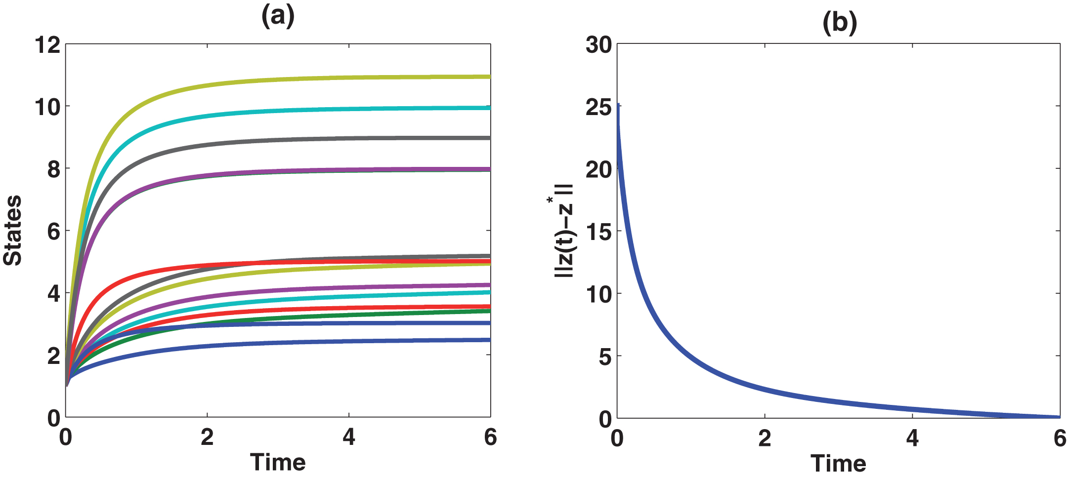
Now, we use the proposed bi-level model (4) and employ the neurodynamic model (15) to solve this problem. All simulation results show the output state trajectory of the neurodynamic model (15) with any initial point is always convergent to z* = (w* T , α* T , β* T ) T . Figure 3(a) displays the phase diagram of state trajectories (x1 (t) , x2 (t)) T of DMU 1 based on (15) with three various initial points and Λ = 1. Figure 4(b) also exhibits the convergence behavior of the error ∥z (t) - z* ∥ 2 with a random initial point and Λ = 1. Table 9 summarizes the results of the bi-level model (4) and the neural network (15). The optimal total revenue is calculated as 1 (2113) +0.1 (2532.48) =2366.248. We see that the total revenue can be increased 43.87% and 0.21% compared with the current total revenue and the total revenue in the Fang and Li’s model (2), respectively. Also, we observe that the minimum reallocation cost of the Fang and Li’s model (3) is equal to ξ* = 226.7662, whereas for the proposed bi-level CRA model (4) we obtain ξ* = 222.63. Furthermore, we compare the proposed model with the Fang and Li’s model in terms of CCR efficiency score. Table 10 gives the comparison results. Like the previous examples, the proposed model has lower average efficiency than the Fang and Li’s model. Therefore, the proposed approach is more suitable for real applications.
At the end of this section, some of the main advantages of the new proposed method compared to the existing ones are summarized below.

(a) Phase diagram of the neurodynamic model (15) with three various initial points and Λ = 1 for inputs of DMU 1 in Example (3), (b) Convergence behavior of the output trajectory norm error based on (15) with a random initial point and Λ = 1 in Example 3.
Results of resources reallocation for 20 DMUs using the proposed bi-level model (4) and the neural network (15) in Example 3
Comparisons of CCR efficiency scores between the two approaches in Example 3
In comparison with the model (1), which aims to maximize the revenue separately for each unit given its input level, the proposed model (4) attempts to maximize the total revenue of all the units by allowing for the reallocation of inputs among the units.
In comparison with the Fang and Li’s (2015) model, which takes the maximum revenue and the minimum reallocation cost using the two-phase procedure (2) and (3) separately, the new method takes the maximum revenue and the minimum reallocation cost simultaneously via the bi-level CRA model (4). However, we observe that the difference of the numerical performance is marginal by testing three illustrative examples. Also, it seems that the results obtained from the proposed model have lower average efficiency. In fact, our model represents a more realistic performance of the units and can reduce the requirements of theranking.
Compared with conventional numerical methods, in devising the proposed neurodynamic model, a properly derived dynamical equation can guarantee that the equilibrium point of the neural network corresponds to the optimal solution of the bi-level CRA problem (4). Also, the neural networks have a fast convergence rate in real-time solutions.
Compared with other existing neural networks for LBPP, the proposed neural network has several merits. First, our neural network model does not depend on the initial points. The reason is that our model is globally convergent to the optimal solution of the problem. Second, the proposed neural network frame (15) can be utilized without a penalty parameter. Third, the structure of the proposed neural network enables a simple circuit implementation.
Modern organizations, especially those operating in centralized decision-making environments have to face with the centralized resource allocation problem. Also, maximizing the total revenue and minimizing the reallocation cost in a hierarchical order can be other goals. In this paper, we extended the classical centralized DEA models to the bi-level CRA models based on revenue efficiency and the cost analysis across a set of DMUs under a centralized decision-making environment. Also, we have designed a gradient neural network for solving the proposed bi-level CRA model. Based on Lyapunov stability theory and LaSalle invariance principle, the proposed neural network has been proved to be globally asymptotically stable and capable of generating the exact optimal solution of the proposed bi-level CRA model. To further demonstrate the advanced features of our approach and its practical relevance, we analyzed various empirical data sets. The results were compared by the Fang and Li’s (2015) model. The achieved results prove the accuracy of the new method. As for further research, it would be interesting to investigate the new bi-level model applications for many other potential organizations with hierarchical structures in transportation, economics, ecology and others.