Parametric sensitivity analysis of linear programming with fuzzy variables

Abstract

Parametric sensitivity analysis is one of the most interesting research topics in linear programming with fuzzy variables (FVLP), and it is also a basic tool for studying perturbations in optimization problems, that is perturbation analysis. The focus of this paper is on two kinds of parametric linear programming with fuzzy variables (PFVLP) which can describe the behaviors of the optimal value under parametric perturbations of the objective function coefficients and the right-hand side of constraint equations in a FVLP, respectively. Firstly, for these two kinds of PFVLP, we investigate how to obtain an optimal basis of them from an optimal basis of their corresponding FVLP based on the parameters in them. Then, two algorithms are proposed to solve these two problems. Finally, two examples are illustrated to show that the PFVLP models proposed in this paper can provide more accurate and scientific suggestions for decision-makers.

Keywords

Parametric sensitivity analysis linear programming with fuzzy variables fuzzy primal and dual simplexalgorithms ranking function trapezoidal fuzzy number

1 Introduction

Since Bellman and Zadeh [1] proposed fuzzy optimization problems in 1970s, a number of researchers have exhibited their interest to solve the fuzzy programming problems for treating uncertainty, especially on fuzzy linear programming (FLP). From a general view, the class of FLP can be broadly classified into four kinds of situations: fuzzy number linear programming (FNLP) [19, 20] in which only the cost coefficients are fuzzy numbers, linear programming with fuzzy variables (FVLP) [14] in which the right-hand-side vector and the decision variables are fuzzy numbers, semi fully fuzzy linear programming (SFFLP) [21, 22] in which the cost coefficients, the right-hand-side vector and the decision variables are fuzzy numbers, and fully fuzzy linear programming (FFLP) [23] in which the cost coefficients, the right- hand-side vector, coefficient matrix and the decision variables are fuzzy numbers.

In recent years, one of the relatively popular topics of FLP is FVLP. Until now, various attempts have been made to study the FVLP problem. To find the optimal solution of FVLP, there exists many methods, such as the simplex methods [2 –5], revised simplex methods [6, 7], penalty method [8], degenerate problem [9, 10] and other special methods [11 –13]. Besides, some scholars also studied the duality of FVLP, such as dual simplex algorithm [14, 15], primal-dual simplex algorithm [16] and some special duality results [17, 18].

Although FLP models permit to represent the flexibility in the values involved in practical problems, one can not stick to all the values for a long time or it is quite possible that the wrong values got entered while a practical problem is formulated as a FLP model. Sensitivity analysis is a basic tool for studying perturbations in optimization problems, which is also one of the interesting research lines in FLP problem [22].

Recently, many scholars studied the sensitivity analysis for FNLP [19, 20], SFFLP [21, 22], FFLP [23] and FVLP [24 –26]. However, sensitivity analysis can only determine the impact of a variable in the model.

In fact, in practical problems, some changes may happen at the same time. Parametric sensitivity analysis can be used to deal with the FLP when some changes occur simultaneously in the cost coefficients and the right-hand-side vector. Kheirfam and Verdegay [21] studied the sensitivity analysis for fuzzy linear programming problems with symmetric trapezoidal fuzzy numbers when the data are perturbed in some cost coefficient ${\tilde{c}}_{k}$ and the right-hand-side vector $\tilde{b}$ , while the fuzzy optimal solution remains invariant. Yanlin Jia etc. [27] studied the parametric sensitivity analysis of objective function in FNLP, in which they proved that if the parameter was in a certain range, the optimal solution remains invariant. However, to the best of our knowledge, till now there is no method in the literature to deal with the parametric sensitivity analysis of FVLP. Parametric sensitivity analysis of FVLP is an extension and supplementary of the sensitivity analysis of FVLP. Based on [21, 27], we will study the problems of parametric sensitivity analysis of objective function and the right-hand side of constraint equation in FVLP in this paper.

This paper is organized as follows: we recall some preliminaries on fuzzy set theory and two existed algorithms to solve the FVLP problems in Section 2. Two kinds of PFVLP models and their corresponding parameter analysis methods are shown in Section 3. Some numerical examples are given in Section 4. Finally, we will allocate the Section 5 to conclusions.

2 Preliminaries

In this section, we recall some necessary concepts, results and operations on fuzzy numbers and ranking function, and some existed methods for solving FVLP, which are needed in the rest of the paper.

A fuzzy set $\tilde{A}$ on R is specified by its membership function $μ_{\tilde{A}}$ , $μ_{\tilde{A}} : R \to [0, 1],$ assigning to each x ∈ R the degree or grade to which x belongs to $\tilde{A}$ . The set ${x \in R : μ_{\tilde{A}} (x) > 0}$ is called the support of $\tilde{A}$ , and the set ${x \in R : μ_{\tilde{A}} (x) = 1}$ is called its kernel.

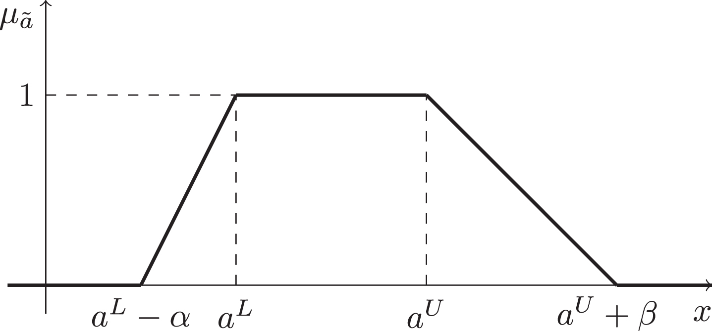
Definition 1. (trapezoidal fuzzy number) [22] A fuzzy number $\tilde{a}$ is said to be a trapezoidal fuzzy number, if there exist real numbers a^L and a^U, a^L ≤ a^U, α > 0 and β > 0, such that $μ_{\tilde{a}} (x) = {\begin{matrix} \frac{x - (a^{L} - α)}{α} & for a^{L} - α \leq x \leq a^{L} \\ 1 & for a^{L} \leq x \leq a^{U} \\ \frac{(a^{U} + β) - x}{β} & for a^{U} \leq x \leq a^{U} + β \\ 0 & else \end{matrix}$

We denote a trapezoidal fuzzy number $\tilde{a}$ by $\tilde{a} = (a^{L}, a^{U}, α, β)$ , where (a^L - α, a^U + β) is the support of $\tilde{a}$ , and [a^L, a^U] is the core of $\tilde{a}$ . $μ_{\tilde{a}} (x)$ is called a membership function of $\tilde{a}$ , and the set of all trapezoidal fuzzy numbers is denoted by F (R). A trapezoidal fuzzy number with the above membership function is shown in Fig. 1.

Fig.1

A trapezoidal fuzzy number.

Definition 2. [28] A fuzzy vector of n dimension is an n-tuple of fuzzy number: $\tilde{c} = ({\tilde{c}}_{1}, {\tilde{c}}_{2}, \dots, {\tilde{c}}_{n})$ , where the fuzzy number ${\tilde{c}}_{i}$ is called the i-th component, 1 ≤ i ≤ n. We denote the set of all fuzzy vectors of n dimension by (F (R)) ⁿ.

Definition 3. (The arithmetic operations on fuzzy numbers) [28] Let $\tilde{a} = (a^{L}, a^{U}, α, β)$ and $\tilde{b} = (b^{L}, b^{U}, γ, θ)$ be two trapezoidal fuzzy numbers. For any x ∈ R,

if x > 0, then $x \tilde{a} = ({xa}^{L}, {xa}^{U}, x α, x β) .$

if x < 0, then $x \tilde{a} = ({xa}^{U}, {xa}^{L}, - x β, - x α) .$

$\tilde{a} + \tilde{b} = (a^{L} + b^{L}, a^{U} + b^{U}, α + γ, β + θ)$ .

Definition 4. [28] Let $\tilde{c} = ({\tilde{c}}_{1}, {\tilde{c}}_{2}, \dots, {\tilde{c}}_{n})$ , $\tilde{d} = ({\tilde{d}}_{1}, {\tilde{d}}_{2}, \dots, {\tilde{d}}_{n})$ be two fuzzy vectors, and a vector k = (k₁, k₂, ⋯ , k_n) ∈ Rⁿ, then

for any x ∈ R, $x \tilde{c} = (x {\tilde{c}}_{1}, x {\tilde{c}}_{2}, \dots, x {\tilde{c}}_{n})$ .

$\tilde{c} + \tilde{d} = ({\tilde{c}}_{1} + {\tilde{d}}_{1}, {\tilde{c}}_{2} + {\tilde{d}}_{2}, \dots, {\tilde{c}}_{n} + {\tilde{d}}_{n})$ .

$k {\tilde{c}}^{T} = k_{1} {\tilde{c}}_{1} + k_{2} {\tilde{c}}_{2} + \dots + k_{n} {\tilde{c}}_{n}$ .

Definition 5. (Ranking function) [14] The function $R : F (R) ⟶ R$ which maps each fuzzy number into the real line is called a ranking function, where a natural order exists.

Definition 6. (Linear ranking function) [14] A ranking function $R : F (R) ⟶ R$ is called a linear ranking function of F (R) into R if it has the following property $R (k \tilde{a} + \tilde{b}) = k R (\tilde{a}) + R (\tilde{b})$ for all $\tilde{a}, \tilde{b} \in F (R)$ , k ∈ R.

Definition 7. [14 , 30] The forms of linear ranking functions on F (R) are considered as follows:

$R (\tilde{a}) = c_{L} a^{L} + c_{U} a^{U} + c_{α} α + c_{β} β$ , where $\tilde{a} = (a^{L}, a^{U}, α, β)$ , and c_L, c_U, c_α, c_β are constants, at least one of which is nonzero.

$R (\tilde{a}) = \frac{1}{2} \int_{0}^{1} (\inf {\tilde{a}}_{λ} + \sup {\tilde{a}}_{λ}) d λ$ , where $\inf {\tilde{a}}_{λ} = a^{L} - α (1 - λ), \sup {\tilde{a}}_{λ} = a^{U} + β (1 - λ)$ in Fig. 1. That is reduced to $R (\tilde{a}) = \frac{a^{L} + a^{U}}{2} + \frac{1}{4} (β - α)$ .

Definition 8. (Orders of ranking function) [14] If $\tilde{a}, \tilde{b} \in F (R)$ , then

$\tilde{a} \underset{R}{\geq} \tilde{b}$ if and only if $R (\tilde{a}) \geq R (\tilde{b})$ .

$\tilde{a} \underset{R}{>} \tilde{b}$ if and only if $R (\tilde{a}) > R (\tilde{b})$ .

$\tilde{a} \underset{R}{=} \tilde{b}$ if and only if $R (\tilde{a}) = R (\tilde{b})$ .

Especially, for any two trapezoidal fuzzy numbers $\tilde{a} = (a^{L}, a^{U}, α, β)$ and $\tilde{b} = (b^{L}, b^{U}, γ, θ)$ , $\tilde{a} \underset{R}{\geq} \tilde{b}$ if and only if $a^{L} + a^{U} + \frac{1}{2} (β - α) \geq b^{L} + b^{U} + \frac{1}{2} (θ - γ)$ .

Definition 9. [28] Let $\tilde{c} = ({\tilde{c}}_{1}, {\tilde{c}}_{2}, \dots, {\tilde{c}}_{n})$ , then ranking function operation of $\tilde{c}$ is defined as $R (\tilde{c}) = (R ({\tilde{c}}_{1}), R ({\tilde{c}}_{2}), . . ., R ({\tilde{c}}_{n})) .$

Definition 10. [14] A FVLP problem defined as follows $\begin{matrix} min & \tilde{z} \underset{R}{=} c \tilde{x} \\ s . t . & A \tilde{x} \underset{R}{=} \tilde{b} \end{matrix}$ (1) $\tilde{x} \underset{R}{\geq} \tilde{0}$ where $\tilde{b} \in (F (R))^{m}, \tilde{x} \in (F (R))^{n}, A \in R^{m \times n}, c^{T} \in R^{n}$ , R (A) = m and $R$ is a linear ranking function.

Especially, if $A \tilde{x} \underset{R}{\leq} \tilde{b}$ in FVLP (1), slack variables $\tilde{y}$ could be added to satisfy $A \tilde{x} + I \tilde{y} \underset{R}{=} \tilde{b}$ . Then the constraint matrix is [A I], where I is the unit matrix.

Let A = [a_ij] _m*n in FVLP (1). Assume rank (A) = m. Partition A as [B N], where B_m*m is nonsingular. It is obvious that rank (B) = m. It is apparent that the basic solution ${\tilde{x}}_{B} = ({\tilde{x}}_{B_{1}}, {\tilde{x}}_{B_{2}}, \dots, {\tilde{x}}_{B_{m}})^{T} = B^{- 1} \tilde{b}, {\tilde{x}}_{N} = \tilde{0}$ is a solution of $A \tilde{x} \underset{R}{=} \tilde{b}$ . If ${\tilde{x}}_{B} \underset{R}{\geq} 0$ , then the fuzzy basic solution is feasible and the corresponding fuzzy objective value is $\tilde{z} \underset{R}{=} c_{B} {\tilde{x}}_{B}$ , where c_B = (c_{B
₁}, c_{B
₂}, ⋯ , c_{B
_m}). There are two existed algorithms to solve the FVLP (1) as following.

Algorithm 1. [5] The fuzzy simplex algorithm for the FVLP problem

Assumption: A basic feasible solution with basis B and the corresponding simplex tableau is at hand.

Step 1: The basic feasible solution is given by ${\tilde{x}}_{B} \underset{R}{=} B^{- 1} \tilde{b}$ and ${\tilde{x}}_{N} \underset{R}{=} \tilde{0}$ . The fuzzy objective value is: $\tilde{z} \underset{R}{=} c_{B} {\tilde{x}}_{B}$ ;

Step 2: Let $z_{k} - c_{k} = max_{j} {z_{j} - c_{j}}, j = 1, \dots, n, j \neq B_{i}, i = 1, \dots, m$ . If z_k - c_k ≤ 0, then stop; the current solution is optimal.

Step 3: If y_k ≤ 0, then stop; the problem is unbounded. Otherwise, determine the index of the variable ${\tilde{x}}_{B_{r}}$ leaving the basis as follows: $\frac{b_{r}}{y_{rk}} = min_{1 \leq i \leq m} {\frac{b_{i}}{y_{ik}} | y_{ik} > 0}$ (2) where $b_{i} = R (B^{- 1} {\tilde{b}}_{i})$ .

Step 4: Pivot on y_rk and update the simplex tableau. Go to Step 2.

Remark 1. If the objective function is maximum, we only need to change the step 2 of Algorithm 1 as following:

Step 2’: Let $z_{k} - c_{k} = min_{j} {z_{j} - c_{j}}, j = 1, \dots, n, j \neq B_{i}, i = 1, \dots, m$ . If z_k - c_k ≥ 0, then stop; the current solution is optimal.

Algorithm 2. [14] the fuzzy dual simplex algorithm for the FVLP problem

Step 1: Given a basis B for the FVLP problem such that z_j - c_j ≤ 0. Compute the fuzzy simplex tableau.

Step 2: If $B^{- 1} \tilde{b} \underset{R}{\geq} \tilde{0}$ , then stop (the current solution is optimal); else select the pivot row r with $B^{- 1} {\tilde{b}}_{r} \underset{R}{<} \tilde{0}$ (that is, r so that $R (B^{- 1} {\tilde{b}}_{r}) < 0$ ).

Step 3: If y_rj ≥ 0 for all j, then stop (the FVLP problem is infeasible); else select the pivot column k by the following minimum ratio test: $\frac{z_{k} - c_{k}}{y_{rk}} = min_{j \neq B_{i}} {\frac{z_{j} - c_{j}}{y_{jk}} ∣ y_{jk} < 0} .$ (3)

Step 4: Pivot on y_rk and go to Step 2.

Remark 2. One suggestion for choice of r in step 2 may be r satisfied $R (B^{- 1} {\tilde{b}}_{r}) = min_{1 \leq i \leq m} {R (B^{- 1} {\tilde{b}}_{i})}$ .

Remark 3. Pivoting on y_rk in step 4 is the usual Gaussian elimination process that, using y_rk, converts column k to the unit vector e_r yielding the new simplex tableau corresponding to the new basis (the one that is obtained by replacing column r of B with a_k).

3 Parametric sensitivity analysis of linear programming with fuzzy variables

In this section, we discuss two problems of parametric perturbations of FVLP (1) which have parameter λ in the coefficients of the objective function and the right hand of the constraints, respectively. Firstly, we investigate how to solve these two problems by making use of the optimal basis of their corresponding FVLP (1). Then, two algorithms are proposed based on ranking function, Algorithms 1 and 2. For convenience, we assume that B is an optimal basis of FVLP (1), and its corresponding optimal solution can be obtained by Algorithms 1 or 2.

3.1 Parameter changes in the coefficients of objective function

The first kind of parametric linear programming with fuzzy variables (PFVLP) discussed in this paper is given as following:

$\begin{matrix} min & \tilde{z} \underset{R}{=} c (λ) \tilde{x} \underset{R}{=} (c + λ c^{'}) \tilde{x} \\ s . t . & A \tilde{x} \underset{R}{=} \tilde{b} \end{matrix}$ (4) $\tilde{x} \underset{R}{\geq} \tilde{0}$ where c^′T ∈ Rⁿ, λ ∈ R is the parameter of variation. Compare with FVLP (1), the fuzzy cost vector of $\tilde{x}$ is changed from c to c + λc′ in PFVLP (4).

Obviously, B is an optimal basis of PFVLP (4) for λ = 0 if B is an optimal basis of FVLP (1). Decomposing A into [B, N], c into [c_B, c_N] and c′ into $[c_{B}^{'}, c_{N}^{'}]$ .

Theorem 1. If FVLP (1) has an optimal basis B, then there exist ${\underline{λ}}_{B}$ and ${\bar{λ}}_{B}$ for PFVLP (4) such that when ${\underline{λ}}_{B} \leq λ \leq {\bar{λ}}_{B}$ , the optimal basis B of FVLP (1) is still an optimal basis for PFVLP (4).

Proof. If λ = 0, PFVLP (4) is equal to FVLP (1). Then the optimal basis is B, the non-basis matrix is N, optimal solution is ${\tilde{x}}_{B} \underset{R}{=} B^{- 1} \tilde{b}, {\tilde{x}}_{N} \underset{R}{=} \tilde{0}$ , and the optimal value is $\tilde{z} \underset{R}{=} c_{B} B^{- 1} \tilde{b}$ .

In PFVLP (4), $c_{B} + λ c_{B}^{'}$ and $c_{N} + λ c_{N}^{'}$ are the coefficients of ${\tilde{x}}_{B}$ and ${\tilde{x}}_{N}$ , respectively.

To prove this conclusion holds, we want to prove that z_j - c_j ≤ 0 of FVLP (4) holds for all j ∈ {1, 2, ⋯ , n} by the Step 2 of Algorithm 1. Therefore, the following optimality conditions must hold: $(c_{B} + λ c_{B}^{'}) B^{- 1} N - (c_{N} + λ c_{N}^{'}) \leq 0$ (5) $λ (c_{B}^{'} B^{- 1} N - c_{N}^{'}) \leq - (c_{B} B^{- 1} N - c_{N})$ (6)

It follows that - (c_BB^-1N - c_N) ≥0 since B is an optimal basis of FVLP (1).

Let $H = c_{B}^{'} B^{- 1} N - c_{N}^{'}$ . Then H must be a vector of n dimension. Now, there are four cases:

Case 1: H = 0_1*n. Obviously, for any λ ∈ R, Equation (6) holds.

Case 2: H > 0_1*n. If Equation (6) holds, then $λ \leq - \frac{(c_{B} B^{- 1} N - c_{N})_{j}}{(c_{B}^{'} B^{- 1} N - c_{N}^{'})_{j}} = - \frac{(c_{B} B^{- 1} N - c_{N})_{j}}{H_{j}}$ (7) for all j ∈ {1, 2, ⋯ , n}, where $H_{j} = (c_{B}^{'} B^{- 1} N - c_{N}^{'})_{j}$ is the j-th component of H.

Case 3: H < 0_1*n. If Equation (6) holds, then $λ \geq - \frac{(c_{B} B^{- 1} N - c_{N})_{j}}{(c_{B}^{'} B^{- 1} N - c_{N}^{'})_{j}}$ (8) for all j ∈ {1, 2, ⋯ , n}.

Case 4: Let P = {p|H_p < 0}, Q = {q|H_q > 0} and Z = {z|H_z = 0}. For any j ∈ P, if Equation (6) holds, then $λ \geq - \frac{(c_{B} B^{- 1} N - c_{N})_{j}}{(c_{B}^{'} B^{- 1} N - c_{N}^{'})_{j}}$ (9)

For any j ∈ Q, if Equation (6) holds, then $λ \leq - \frac{(c_{B} B^{- 1} N - c_{N})_{j}}{(c_{B}^{'} B^{- 1} N - c_{N}^{'})_{j}}$ (10)

For any j ∈ Z, Equation (6) always holds by Case 1.

From the above four cases, if Equation (6) holds, we can obtain Equation (11) as follows. $λ {\begin{matrix} \leq - \frac{(c_{B} B^{- 1} N - c_{N})_{j}}{(c_{B}^{'} B^{- 1} N - c_{N}^{'})_{j}} & if & H_{j} > 0 \\ \geq - \frac{(c_{B} B^{- 1} N - c_{N})_{j}}{(c_{B}^{'} B^{- 1} N - c_{N}^{'})_{j}} & if & H_{j} < 0 \end{matrix}$ (11)

Let ${\bar{λ}}_{B} = {\begin{matrix} min_{j} {- \frac{(c_{B} B^{- 1} N - c_{N})_{j}}{(c_{B}^{'} B^{- 1} N - c_{N}^{'})_{j}} : H_{j} > 0} \\ + \infty : H < 0 \end{matrix}$ (12) ${\underline{λ}}_{B} = {\begin{matrix} max_{j} {- \frac{(c_{B} B^{- 1} N - c_{N})_{j}}{(c_{B}^{'} B^{- 1} N - c_{N}^{'})_{j}} : H_{j} < 0} \\ - \infty : H > 0 \end{matrix}$ (13)

Obviously, ${\bar{λ}}_{B} > 0$ and ${\underline{λ}}_{B} < 0$ .

In summary, if ${\underline{λ}}_{B} \leq λ \leq {\bar{λ}}_{B}$ , Equation (6) holds. The original optimal basis B of FVLP (1) is still optimal to PFVLP (4). Then, the optimal solution is ${\tilde{x}}_{B} \underset{R}{=} B^{- 1} \tilde{b}, {\tilde{x}}_{N} \underset{R}{=} \tilde{0}$ . By the way, the current optimal objective value is $(c_{B} + λ c_{B}^{'}) B^{- 1} \tilde{b} \underset{R}{=} c_{B} B^{- 1} \tilde{b} + λ c_{B}^{'} B^{- 1} \tilde{b} .$ (14)

□

Corollary 1. The optimal objective value of PFVLP (4) is a fuzzy linear function with the parameter λ.

Proof. Immediately from Equation (14) of Theorem 1.

Theorem 2. If $λ > {\bar{λ}}_{B}$ , the original optimal basis B of FVLP (1) is not optimal for PFVLP (4).

Proof. When $λ > {\bar{λ}}_{B}$ , compared with Equation (6), there must exist an index, such that j:

$\begin{matrix} λ (c_{B}^{'} B^{- 1} N - c_{N}^{'})_{j} & > & {\bar{λ}}_{B} (c_{B}^{'} B^{- 1} N - c_{N}^{'})_{j} \\ = & - (c_{B} B^{- 1} N - c_{N})_{j} \end{matrix}$ (15)

By Equation (15), we have $((c_{B} + λ c_{B}^{'}) B^{- 1} N)_{j} - (c_{N} + λ c_{N}^{'})_{j} > 0$ (16)

This implies that z_j - c_j > 0. Hence, the original optimal basis B of FVLP (1) is not optimal for PFVLP (4). Therefore, using Algorithm 1, according to the Step 3, if y_i ≤ 0, PFVLP (4) is unbounded. Otherwise, we can obtain a new optimal basis B′ for PFVLP (4) by Equation (2). □

Remark 4. Given an optimal basis B of FVLP (1), if a new optimal basis B′ of PFVLP (4) with $λ > {\bar{λ}}_{B}$ can be obtained based on B by Algorithm 1, then B′ is an optimal basis of PFVLP (4) with $λ = {\bar{λ}}_{B}$ since z_j - c_j = 0 according to Equation (15). Therefore, if $λ = {\bar{λ}}_{B}$ , then there may exist another optimal basis for FVLP(4) shown in Example 4.1.

Remark 5. The new basis B′ is not optimal basis for PFVLP (4) when $λ < {\bar{λ}}_{B}$ .

Corollary 2. If $λ < {\underline{λ}}_{B}$ , the original optimal basis B of FVLP (1) is not optimal for PFVLP (4).

Proof. Similar to the proof of Theorem 2. □

Remark 6. If $λ = {\underline{λ}}_{B}$ , there may be another new optimal basis to PFVLP (4) besides B.

Remark 7. $λ = {\bar{λ}}_{B}$ and $λ = {\underline{λ}}_{B}$ are the upper and lower breaking point of basis B, respectively.

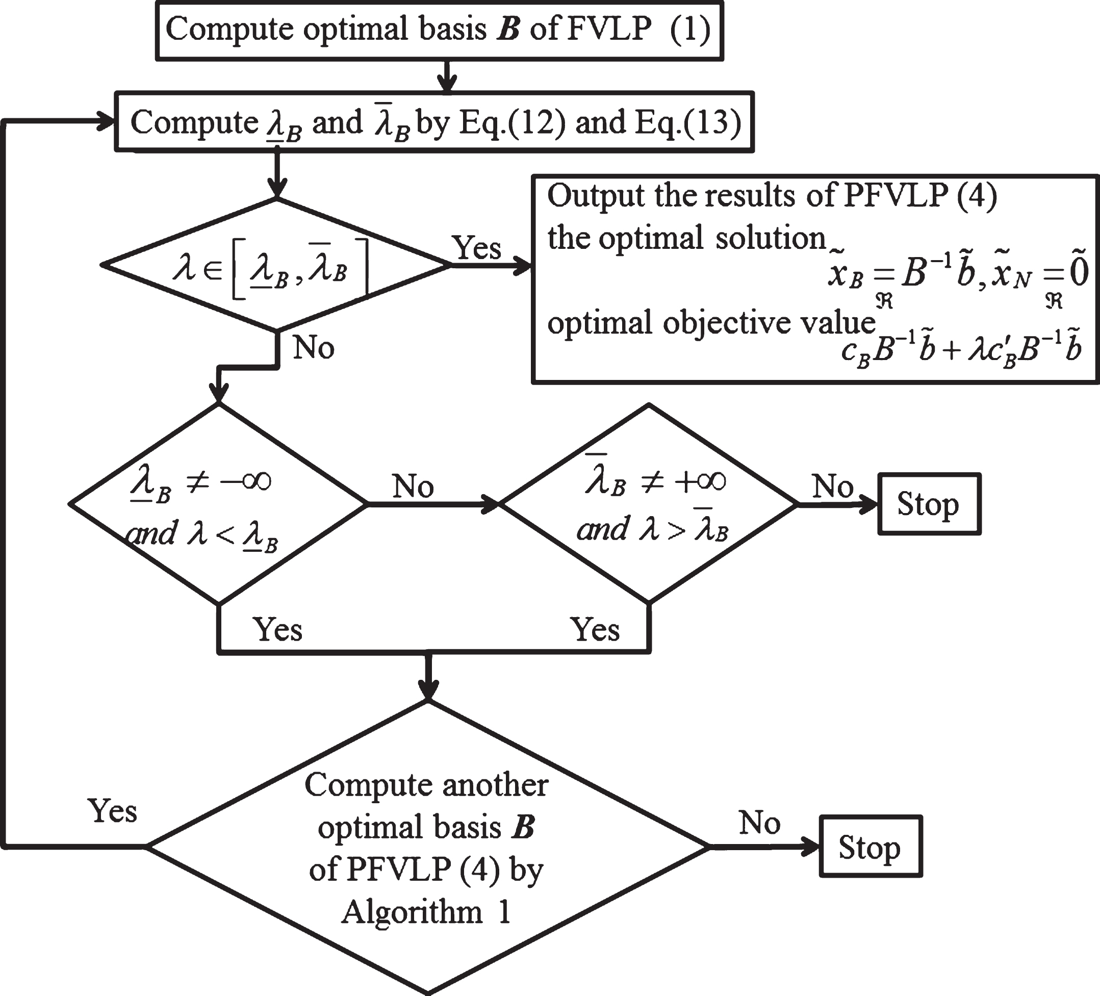
According to Theorems 1, 2 and Algorithm 1, we can propose Algorithm 3 to solve PFVLP(4) for all λ ∈ R, whose flowchart is shown in Fig. 2. We also use Algorithm 3 to solve a practical problem in the later Example 4.1.

Fig.2

Flowchart of Algorithm 3.

Algorithm 3. The parametric sensitivity analysis algorithm to the coefficients of objective function

Assumption: Given a FVLP (1) and its corresponding PFVLP (4), there have an optimal basis B and an optimal simplex tableau of FVLP (1) at hand.

Step 1: According to Equation (12) and Equation (13), compute ${\bar{λ}}_{B}$ and ${\underline{λ}}_{B}$ .

Step 2: If $λ \in [{\underline{λ}}_{B}, {\bar{λ}}_{B}]$ , then compute the optimal solution ${\tilde{x}}_{B} \underset{R}{=} B^{- 1} \tilde{b}, {\tilde{x}}_{N} \underset{R}{=} \tilde{0}$ , optimal objective value $c_{B} B^{- 1} \tilde{b} + λ c_{B}^{'} B^{- 1} \tilde{b}$ and simplex tableau of PFVLP (4). Otherwise, go to the Step 3.

Step 3: If ${\underline{λ}}_{B} \neq - \infty$ and $λ < {\underline{λ}}_{B}$ , then compute the new simplex tableau using Algorithm 1. If there exists a new optimal basis B, then go back to the Step 1. Otherwise, go to the Step 4.

Step 4: If ${\bar{λ}}_{B} \neq + \infty$ and $λ > {\bar{λ}}_{B}$ , then compute the new simplex tableau using Algorithm 1. If there exists a new optimal basis B, then go back to the Step 1. Otherwise, stop.

Remark 8. By Equation (12) and Equation (13), ${\underline{λ}}_{B}$ and ${\bar{λ}}_{B}$ can not be infinite at the same time in the judge statement $λ \in [{\underline{λ}}_{B}, {\bar{λ}}_{B}]$ of Fig. 2. Furthermore, λ is always finite. Therefore, we can regardless of whether there is an infinity in the step 2 of Algorithm 3.

3.2 Parameter changes in the right hand of the constraints

The second kind of parametric linear programming with fuzzy variables (PFVLP) discussed in this paper is given as the following: $\begin{matrix} min & \tilde{z} \underset{R}{=} c \tilde{x} \\ s . t . & A \tilde{x} \underset{R}{=} \tilde{b} (λ) \underset{R}{=} \tilde{b} + λ {\tilde{b}}^{'} \end{matrix}$ (17) $\tilde{x} \underset{R}{\geq} \tilde{0}$ where ${\tilde{b}}^{'} \in (F (R))^{m}$ , λ ∈ R is the parameter of variation. Compared with FVLP (1), the right hand of the constraints are changed from $\tilde{b}$ to $\tilde{b} (λ) \underset{R}{=} \tilde{b} + λ {\tilde{b}}^{'}$ in PFVLP (17).

Obviously, B is an optimal basis of PFVLP (17) for λ = 0. Decomposing A into [B, N], c into [c_B, c_N].

Theorem 3. If FVLP (1) has an optimal basis B, then there exist ${\underline{λ}}_{B}$ and ${\bar{λ}}_{B}$ for PFVLP (17), such that when ${\underline{λ}}_{B} \leq λ \leq {\bar{λ}}_{B}$ , B is still optimal for PFVLP (17).

Proof. If λ = 0, PFVLP (17) is equal to FVLP (1). Hence, the optimal basis is B, the non-basis matrix is N, optimal solution is ${\tilde{x}}_{B} \underset{R}{=} B^{- 1} \tilde{b}, {\tilde{x}}_{N} \underset{R}{=} \tilde{0}$ , and the optimal value is $\tilde{z} \underset{R}{=} c_{B} B^{- 1} \tilde{b}$ .

To prove the original optimal basis B of FVLP (1) preserves optimality to PFVLP (17), we want to prove the current solution of PFVLP (17) ${\tilde{x}}_{B} \underset{R}{=} B^{- 1} \tilde{b} + λ B^{- 1} {\tilde{b}}^{'}, {\tilde{x}}_{N} \underset{R}{=} \tilde{0}$ is optimal. Therefore, Equation (18) must hold by the Step 2 of Algorithm 2. ${\tilde{x}}_{B} \underset{R}{=} B^{- 1} \tilde{b} + λ B^{- 1} {\tilde{b}}^{'} \underset{R}{\geq} \tilde{0}, {\tilde{x}}_{N} \underset{R}{=} \tilde{0}$ (18)

By Definition 8, the Equation (18) is equivalent to Equation (19). $R (B^{- 1} \tilde{b}) + λ R (B^{- 1} {\tilde{b}}^{'}) \geq 0, R ({\tilde{x}}_{N}) = 0$ (19)

It follows that $R (B^{- 1} \tilde{b}) \geq 0$ in Equation (19) since B is an optimal basis of FVLP (1).

Let $V = R (B^{- 1} {\tilde{b}}^{'})$ . Then, by Definition 9, V must be a vector of m dimension. Now, there are four cases:

Case 1: V = 0_m*1. Obviously, for any λ ∈ R, Equation (19) holds.

Case 2: V > 0_m*1. If Equation (19) holds, then $λ \geq - \frac{(R (B^{- 1} \tilde{b}))_{i}}{(R (B^{- 1} {\tilde{b}}^{'}))_{i}} = - \frac{(R (B^{- 1} \tilde{b}))_{i}}{V_{i}}$ (20) for all i ∈ {1, 2, ⋯ , m}, where $V_{i} = (R (B^{- 1} {\tilde{b}}^{'}))_{i}$ is the i-th component of V.

Case 3: V < 0_m*1. If Equation (19) holds, then $λ \leq - \frac{(R (B^{- 1} \tilde{b}))_{i}}{(R (B^{- 1} {\tilde{b}}^{'}))_{i}}$ (21) for all i ∈ {1, 2, ⋯ , m}.

Case 4: Let P = {p|V_p < 0}, Q = {q|V_q > 0} and Z = {z|V_z = 0}. For any i ∈ P, if Equation (19) holds, then $λ \leq - \frac{(R (B^{- 1} \tilde{b}))_{i}}{(R (B^{- 1} {\tilde{b}}^{'}))_{i}}$ (22)

For any i ∈ Q, if Equation (19) holds, then

$λ \geq - \frac{(R (B^{- 1} \tilde{b}))_{i}}{(R (B^{- 1} {\tilde{b}}^{'}))_{i}}$ (23)

For any i ∈ Z, Equation (19) always hold by Case 1.

From the above four cases, if Equation (19) holds, we can obtain Equation (24) as follows. $λ {\begin{matrix} \geq - \frac{(R (B^{- 1} \tilde{b}))_{i}}{(R (B^{- 1} {\tilde{b}}^{'}))_{i}} & if & V_{i} > 0 \\ \leq - \frac{(R (B^{- 1} \tilde{b}))_{i}}{(R (B^{- 1} {\tilde{b}}^{'}))_{i}} & if & V_{i} < 0 \end{matrix}$ (24)

Let ${\bar{λ}}_{B} = {\begin{matrix} min {- \frac{(R (B^{- 1} \tilde{b}))_{i}}{(R (B^{- 1} {\tilde{b}}^{'}))_{i}} : V_{i} < 0} \\ + \infty : H > 0 \end{matrix}$ (25) ${\underline{λ}}_{B} = {\begin{matrix} max {- \frac{(R (B^{- 1} \tilde{b}))_{i}}{(R (B^{- 1} {\tilde{b}}^{'}))_{i}} : V_{i} > 0} \\ - \infty : H < 0 \end{matrix}$ (26)

Obviously, ${\bar{λ}}_{B} > 0$ and ${\underline{λ}}_{B} < 0$ .

In summary, if ${\underline{λ}}_{B} \leq λ \leq {\bar{λ}}_{B}$ , Equation (19) holds. The original optimal basis B of FVLP (1) is still optimal to PFVLP (17). But the current optimal solution of PFVLP (17) is ${\tilde{x}}_{B} \underset{R}{=} B^{- 1} \tilde{b} + λ B^{- 1} {\tilde{b}}^{'}, {\tilde{x}}_{N} \underset{R}{=} \tilde{0}$ . By the way, the current optimal objective value is $c_{B} B^{- 1} \tilde{b} (λ) \underset{R}{=} c_{B} B^{- 1} \tilde{b} + λ c_{B} B^{- 1} {\tilde{b}}^{'} .$ (27)

□

Corollary 3. The optimal objective value of PFVLP (17) is a fuzzy linear function with the parameter λ.

Proof. Immediately from Equation (27) of Theorem 3. □

Theorem 4. If $λ > {\bar{λ}}_{B}$ , then the original optimal basis B of FVLP (1) is not optimal to PFVLP (17), but there must be a new optimal basis B′ for PFVLP (17) if PFVLP (17) is feasible.

Proof. If $λ > {\bar{λ}}_{B}$ , compared with Equation (19), there must exist an index i:

$\begin{matrix} (R (B^{- 1} \tilde{b}))_{i} + λ (R (B^{- 1} {\tilde{b}}^{'}))_{i} \\ < (R (B^{- 1} \tilde{b}))_{i} + λ_{B} (R (B^{- 1} {\tilde{b}}^{'}))_{i} = 0 \end{matrix}$ (28)

Therefore, using Algorithm 2, by the Step 2, let r = i be the pivot row. And according to the Step 3, if y_rj ≥ 0 for all j, the PFVLP (17) is infeasible. Otherwise, we can get a new optimal basis B′ for PFVLP (17) by Equation (3). That is, the original optimal basis B of FVLP (1) is not optimal to PFVLP (17). □

Remark 9. Given an optimal basis B of FVLP (1), if a new optimal basis B′ of PFVLP (17) with $λ > {\bar{λ}}_{B}$ can be obtained based on B by Algorithm 2, then B′ is an optimal basis of PFVLP (17) with $λ = {\bar{λ}}_{B}$ since $(R (B^{- 1} \tilde{b}))_{i} + λ (R (B^{- 1} {\tilde{b}}^{'}))_{i} = (R (B^{- 1} \tilde{b}))_{i} + {\bar{λ}}_{B} (R (B^{- 1} {\tilde{b}}^{'}))_{i} = 0$ according to Equation (28). Therefore, if $λ = {\bar{λ}}_{B}$ , then there may exist another optimal basis for PFVLP(17) shown in Example 4.2.

Remark 10. The new basis B′ is not optimal basis when $λ < {\bar{λ}}_{B}$ .

Corollary 4. If $λ < {\underline{λ}}_{B}$ , then the original optimal basis B of FVLP (1) is not optimal to PFVLP (17), but there must be a new optimal basis B″ for PFVLP (17) if PFVLP (17) is feasible.

Proof. Similar to the proof of Theorem 4. □

Remark 11. If $λ = {\underline{λ}}_{B}$ , there may be another new optimal basis to PFVLP (17) besides B.

Remark 12. $λ = {\bar{λ}}_{B}$ and $λ = {\underline{λ}}_{B}$ are the upper and lower breaking point of basis B, respectively.

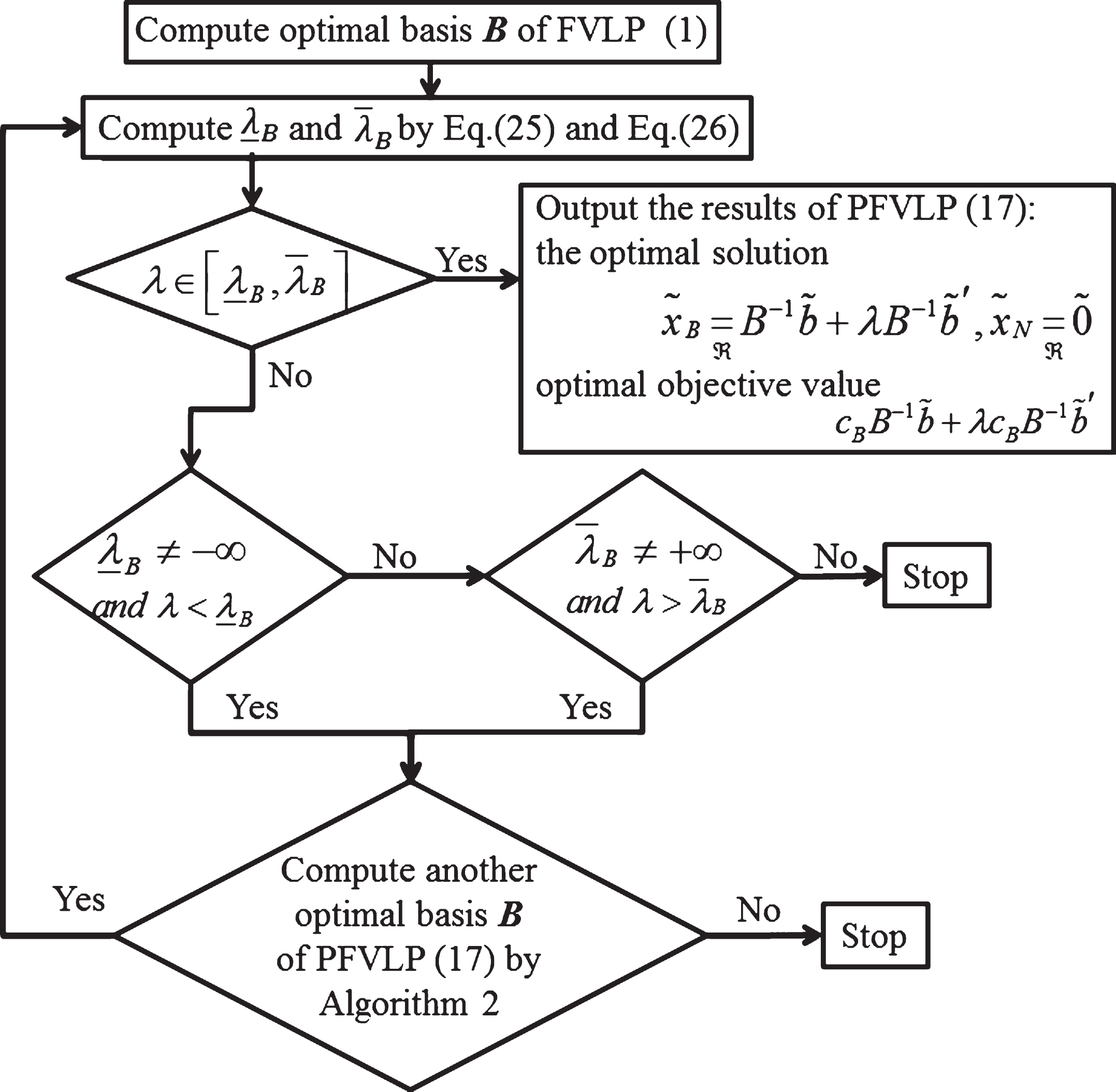
According to Theorems 3, 4 and Algorithm 2, we can propose Algorithm 4 to solve PFVLP (17) for all λ ∈ R, whose flowchart is shown in Fig. 3. We also use Algorithm 4 to solve a practical problem in the later Example 4.2.

Fig.3

Flowchart of Algorithm 4.

Algorithm 4. The parametric sensitivity analysis algorithm to the right hand of the constraints

Assumption: Given a FVLP (1) and its corresponding PFVLP (17), there have an optimal basis B and an optimal simplex tableau of FVLP (1) at hand.

Step 1: According to Equation (25) and Equation (26), compute ${\bar{λ}}_{B}$ and ${\underline{λ}}_{B}$ .

Step 2: If $λ \in [{\underline{λ}}_{B}, {\bar{λ}}_{B}]$ , then compute the optimal solution ${\tilde{x}}_{B} \underset{R}{=} B^{- 1} \tilde{b} + λ B^{- 1} {\tilde{b}}^{'}, {\tilde{x}}_{N} \underset{R}{=} \tilde{0}$ , optimal objective value $c_{B} B^{- 1} \tilde{b} + λ c_{B} B^{- 1} {\tilde{b}}^{'}$ and simplex tableau of PFVLP (17). Otherwise, go to the Step 3.

Step 3: If ${\underline{λ}}_{B} \neq - \infty$ and $λ < {\underline{λ}}_{B}$ , then compute the new simplex tableau using Algorithm 2. If there exists a new optimal basis B, then go back to the Step 1. Otherwise, go to the Step 4.

Step 4: If ${\bar{λ}}_{B} \neq + \infty$ and $λ > {\bar{λ}}_{B}$ , then compute the new simplex tableau using Algorithm 2. If there exists a new optimal basis B, then go back to the Step 1. Otherwise, stop.

Remark 13. By Equation (25) and Equation (26), ${\underline{λ}}_{B}$ and ${\bar{λ}}_{B}$ can not be infinite at the same time in the judge statement $λ \in [{\underline{λ}}_{B}, {\bar{λ}}_{B}]$ of Fig. 3. Furthermore, λ is always finite. Therefore, we can regardless of whether there is an infinity in the step 2 of Algorithm 4.

4 Numerical example

In this section, two numerical examples are illustrated to show how to solve the two kinds of PFVLP proposed in this paper by Algorithms 3 and 4.

Question 1: A factory produces two products representing with P1 and P2, which are made by manual system and machine system a day. The detailed relationship between production capacity and pure profit is shown in Table 1. The daily capacity of two systems for the products P1 and P2 is about 8 and 7 hours, respectively. So how to arrange the production to get the maximum pure profit?

Table 1
The relationship among daily capacity, time per unit of each production and pure profit

System Daily capacity Time per unit Pure

P1 P2 Profit

Manual (7, 9, 0.2, 1) 3 1 3

Machine (6.8, 7.2, 0.1, 1) 1 2 5

System	Daily capacity	Time per unit	Pure
Manual	(7, 9, 0.2, 1)	3	1	3
Machine	(6.8, 7.2, 0.1, 1)	1	2	5

Remark 14. (1) In Table 1, the measure unit of daily capacity is hour, the measure unit of Time is hour per unit, and the measure unit of pure profit is thousand dollars per unit.

(2) In Table 1, daily capacity of each system is fuzzy. If its daily capacity is about 8 after investigation, then it may be presented as a trapezoidal fuzzy number. That is (7, 9, 0.2, 1).

(3) The production for each system can vary due to variations in other condition, such as physical qualifications, manpower resource, technological innovation. So we can use a trapezoidal fuzzy number to denote the range of the production after investigation.

Solution: Let x₁ and x₂ denote daily amount of P1 and P2, respectively. In this case, the problem is formulated as the following FVLP (29). $\begin{matrix} max & \tilde{z} \underset{R}{=} 3 {\tilde{x}}_{1} + 5 {\tilde{x}}_{2} \\ s . t . & 3 {\tilde{x}}_{1} + {\tilde{x}}_{2} \underset{R}{\leq} (7, 9, 0.2, 1) \\ {\tilde{x}}_{1} + 2 {\tilde{x}}_{2} \underset{R}{\leq} (6.8, 7.2, 0.1, 1) \end{matrix}$ (29) $x_{j} \geq 0, j = 1, 2 .$

Adding the slack variables and minimizing the objective function, we have the following FVLP (30).

$\begin{matrix} min & {\tilde{z}}^{'} \underset{R}{=} - \tilde{z} \underset{R}{=} - 3 {\tilde{x}}_{1} - 5 {\tilde{x}}_{2} \\ s . t . & 3 {\tilde{x}}_{1} + {\tilde{x}}_{2} + {\tilde{x}}_{3} \underset{R}{=} (7, 9, 0.2, 1) \\ {\tilde{x}}_{1} + 2 {\tilde{x}}_{2} + {\tilde{x}}_{4} \underset{R}{=} (6.8, 7.2, 0.1, 1) \\ x_{j} \geq 0, j = 1, \cdot \cdot \cdot, 4 . \end{matrix}$ (30)

Next, using the Algorithm 1, after two times iteration, the final simplex tableau of FVLP (30) is given in Table 2.

Table 2

Final simplex tableau of FVLP (30)

	${\tilde{x}}_{1}$	${\tilde{x}}_{2}$	${\tilde{x}}_{3}$	${\tilde{x}}_{4}$	$\tilde{b}$
${\tilde{x}}_{1}$	1	0	$\frac{2}{5}$	$- \frac{1}{5}$	$(\frac{34}{25}, \frac{56}{25}, \frac{7}{25}, \frac{21}{50})$
${\tilde{x}}_{2}$	0	1	$- \frac{1}{5}$	$\frac{3}{5}$	$(\frac{57}{25}, \frac{73}{25}, \frac{13}{50}, \frac{16}{25})$
	0	0	$- \frac{1}{5}$	$- \frac{12}{5}$	$- (\frac{442}{25}, \frac{478}{25}, \frac{39}{100}, \frac{271}{100})$

Example 4.1. Consider the Question 1. Due to some objective reasons, such as economic policy, seasonal changes, the profits of P1 and P2 change. After investigation, the profits of products is c + λc′ = (3, 5) + λ (1, - 1), a function of λ. That is, the profits of products are perturbed along the profit vector c′ = (1, - 1).

In fact, we should solve the following PFVLP (31), which belongs to the first kind of parametric linear programming with fuzzy variables. $\begin{matrix} min & {\tilde{z}}^{'} \underset{R}{=} - (3 + λ) {\tilde{x}}_{1} - (5 - λ) {\tilde{x}}_{2} \\ s . t . & 3 {\tilde{x}}_{1} + {\tilde{x}}_{2} + {\tilde{x}}_{3} \underset{R}{=} (7, 9, 0.2, 1) \\ {\tilde{x}}_{1} + 2 {\tilde{x}}_{2} + {\tilde{x}}_{4} \underset{R}{=} (6.8, 7.2, 0.1, 1) \end{matrix}$ (31) $x_{j} \geq 0, j = 1, \cdot \cdot \cdot, 4 .$

Then, a parameter λ changes in the coefficients of objective function. We only need to modify the last row of Table 2. According to Equation (5), we only consider the number $z_{k}^{'} - c_{k}$ for k = 3, 4. Hence $\begin{matrix} c_{B}^{'} B^{- 1} N - c_{N}^{'} & = & c_{B}^{'} (y_{3}, y_{4}) - (c_{3}, c_{4}) \\ = & (\begin{matrix} - 1 & 1 \end{matrix}) (\begin{matrix} \frac{2}{5} & - \frac{1}{5} \\ - \frac{1}{5} & \frac{3}{5} \end{matrix}) - (\begin{matrix} 0 & 0 \end{matrix}) \\ = & (\begin{matrix} - \frac{3}{5} & \frac{4}{5} \end{matrix}) \end{matrix}$

Therefore, the number $z_{k}^{'} - c_{k}$ for k = 3, 4 is $\begin{matrix} (c_{B} + λ c_{B}^{'}) B^{- 1} N - (c_{N} + λ c_{N}^{'}) \\ = (\begin{matrix} - \frac{1}{5} - \frac{3}{5} λ & - \frac{12}{5} + \frac{4}{5} λ \end{matrix}) \end{matrix}$ and the optimal value is $\begin{matrix} (c_{B} + λ c_{B}^{'}) {\tilde{x}}_{B} \\ \underset{R}{=} (\begin{matrix} - 3 - λ & - 5 + λ \end{matrix}) (\begin{matrix} (\frac{34}{25}, \frac{56}{25}, \frac{7}{25}, \frac{21}{50}) \\ (\frac{57}{25}, \frac{73}{25}, \frac{13}{50}, \frac{16}{25}) \end{matrix}) \\ \underset{R}{=} - (\frac{442}{25}, \frac{478}{25}, \frac{39}{100}, \frac{271}{100}) \\ + λ (\frac{1}{25}, \frac{39}{25}, \frac{17}{25}, \frac{23}{25}) \end{matrix}$

According to Equations (12) and (13), ${\bar{λ}}_{1} = - (- \frac{12}{5}) / (\frac{4}{5}) = 3$ and ${\underline{λ}}_{1} = - (- \frac{1}{5}) / (- \frac{3}{5}) = - \frac{1}{3} .$

Therefore, B remains optimal and feasible for $λ \in [{\underline{λ}}_{1}, {\bar{λ}}_{1}] = [- \frac{1}{3}, 3]$ . The optimal solution is $\begin{matrix} ({\tilde{x}}_{1}, {\tilde{x}}_{2}) \\ = ((\frac{34}{25}, \frac{56}{25}, \frac{7}{25}, \frac{21}{50}), (\frac{57}{25}, \frac{73}{25}, \frac{13}{50}, \frac{16}{25})) \end{matrix}$ and the optimal value is $- (\frac{442}{25}, \frac{478}{25}, \frac{39}{100}, \frac{271}{100}) + λ (\frac{1}{25}, \frac{39}{25}, \frac{17}{25}, \frac{23}{25}) .$

The current optimal simplex table is given in Table 3.

Table 3

Optimal simplex tableau of PFVLP (31) when $λ \in [- \frac{1}{3}, 3]$

	${\tilde{x}}_{1}$	${\tilde{x}}_{2}$	${\tilde{x}}_{3}$	${\tilde{x}}_{4}$	$\tilde{b}$
${\tilde{x}}_{1}$	1	0	$\frac{2}{5}$	$- \frac{1}{5}$	$(\frac{34}{25}, \frac{56}{25}, \frac{7}{25}, \frac{21}{50})$
${\tilde{x}}_{2}$	0	1	$- \frac{1}{5}$	$\frac{3}{5}$	$(\frac{57}{25}, \frac{73}{25}, \frac{13}{50}, \frac{16}{25})$
	0	0	$- \frac{1}{5} - \frac{3}{5} λ$	$- \frac{12}{5} + \frac{4}{5} λ$	$- (\frac{442}{25}, \frac{478}{25}, \frac{39}{100}, \frac{271}{100}) + λ (\frac{1}{25}, \frac{39}{25}, \frac{17}{25}, \frac{23}{25})$

If λ > 3, the original basis is not optimal. Then ${\tilde{x}}_{4}$ enters the basis and the leaving variable is ${\tilde{x}}_{2}$ . The optimal simplex table is given in Table 4.

Table 4

Optimal simplex tableau of of PFVLP (31) when λ > 3

	${\tilde{x}}_{1}$	${\tilde{x}}_{2}$	${\tilde{x}}_{3}$	${\tilde{x}}_{4}$	$\tilde{b}$
${\tilde{x}}_{1}$	1	$\frac{1}{3}$	$\frac{1}{3}$	0	$(\frac{53}{25}, \frac{241}{75}, \frac{11}{30}, \frac{19}{30})$
${\tilde{x}}_{4}$	0	$\frac{5}{3}$	$- \frac{1}{3}$	1	$(\frac{19}{5}, \frac{73}{15}, \frac{13}{30}, \frac{16}{15})$
	0	$4 - \frac{4}{3} λ$	$- 1 - \frac{1}{3} λ$	0	$(- 10, - 6, \frac{15}{4}, \frac{59}{20}) + λ (- \frac{289}{75}, - \frac{37}{25}, \frac{23}{15}, \frac{19}{15})$

Next, according to Equations (12) and (13), ${\bar{λ}}_{2} = + \infty$ and ${\underline{λ}}_{2} = \max {- \frac{4}{- \frac{4}{3}}, - \frac{- 1}{- \frac{1}{3}}} = 3 .$

Hence, when λ ≥ 3, the new basic is B′ = [x₁, x₄], the optimal solution is $({\tilde{x}}_{1}, {\tilde{x}}_{2}) \underset{R}{=} ((\frac{53}{25}, \frac{241}{75}, \frac{11}{30}, \frac{19}{30}), \tilde{0})$ and the optimal value is $(- 10, - 6, \frac{15}{4}, \frac{59}{20}) + λ (- \frac{289}{75}, - \frac{37}{25}, \frac{23}{15}, \frac{19}{15}) .$

That is, if λ ≥ 3, the decision maker should only produce P1.

By the way, obviously, when λ ≥ 5, the decision maker should stop producing P2 since the pure profit of P2 is less than zero. In a sense, PFVLP (31) can provide a more accurate plan for decision-makers since our suggestion is that when λ ≥ 3, stop producing P2.

If $λ < - \frac{1}{3}$ , the original basis is not optimal. Then ${\tilde{x}}_{3}$ enters the basis and the leaving variable is ${\tilde{x}}_{1}$ . The optimal simplex table is given in Table 5.

Table 5

Optimal simplex tableau of of PFVLP (31) when $λ < - \frac{1}{3}$

	${\tilde{x}}_{1}$	${\tilde{x}}_{2}$	${\tilde{x}}_{3}$	${\tilde{x}}_{4}$	$\tilde{b}$
${\tilde{x}}_{3}$	$\frac{5}{2}$	0	1	$- \frac{1}{2}$	$(\frac{17}{5}, \frac{28}{5}, \frac{7}{10}, \frac{21}{20})$
${\tilde{x}}_{2}$	$\frac{1}{2}$	1	0	$\frac{1}{2}$	$(\frac{74}{25}, \frac{101}{25}, \frac{2}{5}, \frac{17}{20})$
	$\frac{1}{2} + \frac{3}{2} λ$	0	0	$- \frac{5}{2} + \frac{1}{2} λ$	$(- \frac{461}{25}, - \frac{414}{25}, \frac{57}{20}, \frac{3}{5}) + λ (\frac{52}{25}, \frac{123}{25}, \frac{11}{10}, \frac{31}{20})$

Next, according to Equations (12) and (13), ${\bar{λ}}_{3} = \min {- \frac{\frac{1}{2}}{\frac{3}{2}}, - \frac{- \frac{5}{2}}{\frac{1}{2}}} = - \frac{1}{3}$ and ${\underline{λ}}_{3} = - \infty .$

Therefore, if $λ \leq - \frac{1}{3}$ , the new basic is B′ = [x₃, x₂], the optimal solution is $({\tilde{x}}_{1}, {\tilde{x}}_{2}) \underset{R}{=} (\tilde{0}, (\frac{74}{25}, \frac{101}{25}, \frac{2}{5}, \frac{17}{20}))$ and the optimal value is

$(- \frac{461}{25}, - \frac{414}{25}, \frac{57}{20}, \frac{3}{5}) + λ (\frac{52}{25}, \frac{123}{25}, \frac{11}{10}, \frac{31}{20}) .$

That is, if $λ \leq - \frac{1}{3}$ , the decision maker should only produce P2.

By the way, obviously, if λ ≤ -3, the decision maker should stop producing P1 since the pure profit of P1 is less than zero. In a sense, PFVLP (31) can provide a more accurate plan for decision-makers since our suggestion is that when $λ \leq - \frac{1}{3}$ , stop producing P1.

To sum up, the optimal solution for the entire range of λ is summarized in Table 6. The value of object function is computed by direct substitution.

Table 6

The optimal solutions with different parameter λ of PFVLP (31)

λ	${\tilde{x}}_{1}$	${\tilde{x}}_{2}$	${\tilde{z}}^{'} \underset{R}{=} - \tilde{z}$
$[- \frac{1}{3}, 3]$	$(\frac{34}{25}, \frac{56}{25}, \frac{7}{25}, \frac{21}{50})$	$(\frac{57}{25}, \frac{73}{25}, \frac{13}{50}, \frac{16}{25})$	$- (\frac{442}{25}, \frac{478}{25}, \frac{39}{100}, \frac{271}{100}) + λ (\frac{1}{25}, \frac{39}{25}, \frac{17}{25}, \frac{23}{25})$
[3, + ∞]	$(\frac{53}{25}, \frac{241}{75}, \frac{11}{30}, \frac{19}{30})$	$\tilde{0}$	$(- 10, - 6, \frac{15}{4}, \frac{59}{20}) + λ (- \frac{289}{75}, - \frac{37}{25}, \frac{23}{15}, \frac{19}{15})$
$(- \infty, - \frac{1}{3}]$	$\tilde{0}$	$(\frac{74}{25}, \frac{101}{25}, \frac{2}{5}, \frac{17}{20})$	$(- \frac{461}{25}, - \frac{414}{25}, \frac{57}{20}, \frac{3}{5}) + λ (\frac{52}{25}, \frac{123}{25}, \frac{11}{10}, \frac{31}{20})$

Example 4.2. Also consider the Question 1. Due to some objective reasons, such as manpower resource, technological innovation, the daily capacity of manual system and machine system changes. After investigation, the daily capacity of manual system and machine system is $\tilde{b} + λ {\tilde{b}}^{'} = ((7, 9, 0.2, 1), (6.8, 7.2, 0.1, 1)) + λ (- (1, 2, 0.2, 0.2), (1, 2, 0.2, 0.2))$ , a function of λ. That is, the daily capacity of manual system and machine system is perturbed along the right-hand-side vector ${\tilde{b}}^{'} = ((- 2, - 1, 0.2, 0.2), (1, 2, 0.2, 0.2))$ .

Compared with FVLP (30), we should solve the following PFVLP (32), which belongs to the second kind of parametric linear programming with fuzzy variables.

$\begin{matrix} min & {\tilde{z}}^{'} \underset{R}{=} - 3 {\tilde{x}}_{1} - 5 {\tilde{x}}_{2} \\ s . t . & 3 {\tilde{x}}_{1} + {\tilde{x}}_{2} + {\tilde{x}}_{3} \underset{R}{=} (7, 9, 0.2, 1) \\ - λ (1, 2, 0.2, 0.2) \\ {\tilde{x}}_{1} + 2 {\tilde{x}}_{2} + {\tilde{x}}_{4} \underset{R}{=} (6.8, 7.2, 0.1, 1) \\ + λ (1, 2, 0.2, 0.2) \\ x_{j} \geq 0, j = 1, \cdot \cdot \cdot, 4 . \end{matrix}$ (32)

Then, a parameter λ changes in the right hand of the constraints. We only need to modify the last column of Table 2. Hence, $\begin{matrix} {\tilde{x}}_{B} & \underset{R}{=} & (\begin{matrix} {\tilde{x}}_{2} \\ {\tilde{x}}_{1} \end{matrix}) \underset{R}{=} B^{- 1} \tilde{b} + λ B^{- 1} {\tilde{b}}^{'} \\ \underset{R}{=} & (\begin{matrix} (\frac{34}{25}, \frac{56}{25}, \frac{7}{25}, \frac{21}{50}) \\ (\frac{57}{25}, \frac{73}{25}, \frac{13}{50}, \frac{16}{25}) \end{matrix}) \\ + (\begin{matrix} \frac{2}{5} & - \frac{1}{5} \\ - \frac{1}{5} & \frac{3}{5} \end{matrix}) (\begin{matrix} (- 2, - 1, 0.2, 0.2) \\ (1, 2, 0.2, 0.2) \end{matrix}) λ \\ \underset{R}{=} & (\begin{matrix} (\frac{34}{25}, \frac{56}{25}, \frac{7}{25}, \frac{21}{50}) + λ (- \frac{6}{5}, - \frac{3}{5}, \frac{3}{25}, \frac{3}{25}) \\ (\frac{57}{25}, \frac{73}{25}, \frac{13}{50}, \frac{16}{25}) + λ (\frac{4}{5}, \frac{8}{5}, \frac{4}{25}, \frac{4}{25}) \end{matrix}) \end{matrix}$

According to Equations (25) and (26), $\begin{matrix} {\bar{λ}}_{1} & = & min {- \frac{R ((\frac{34}{25}, \frac{56}{25}, \frac{7}{25}, \frac{21}{50}))}{R ((- \frac{6}{5}, - \frac{3}{5}, \frac{3}{25}, \frac{3}{25}))}} \\ = & min {- \frac{\frac{367}{200}}{(- \frac{9}{10})}} = \frac{367}{180} \end{matrix}$ and $\begin{matrix} {\underline{λ}}_{1} & = & min {- \frac{R ((\frac{57}{25}, \frac{73}{25}, \frac{13}{50}, \frac{16}{25}))}{R ((\frac{4}{5}, \frac{8}{5}, \frac{4}{25}, \frac{4}{25}))}} \\ = & min {- \frac{\frac{539}{200}}{\frac{6}{5}}} = - \frac{539}{240} . \end{matrix}$

Therefore, B remains optimal and feasible for $λ \in [- \frac{539}{240}, \frac{367}{180}]$ . The optimal solution is $\begin{matrix} ({\tilde{x}}_{1}, {\tilde{x}}_{2}) \\ \underset{R}{=} ((\frac{34}{25}, \frac{56}{25}, \frac{7}{25}, \frac{21}{50}) + λ (- \frac{6}{5}, - \frac{3}{5}, \frac{3}{25}, \frac{3}{25}), \\ (\frac{57}{25}, \frac{73}{25}, \frac{13}{50}, \frac{16}{25}) + λ (\frac{4}{5}, \frac{8}{5}, \frac{4}{25}, \frac{4}{25})) \end{matrix}$ and the optimal value is $\begin{matrix} - (\frac{442}{25}, \frac{478}{25}, \frac{39}{100}, \frac{271}{100}) \\ + λ (- \frac{31}{5}, - \frac{2}{5}, \frac{29}{25}, \frac{29}{25}) . \end{matrix}$

The optimal simplex table is given in Table 7.

Table 7

Optimal simplex tableau of PFVLP (32) when $λ \in [- \frac{539}{240}, \frac{367}{180}]$

	${\tilde{x}}_{1}$	${\tilde{x}}_{2}$	${\tilde{x}}_{3}$	${\tilde{x}}_{4}$	$\tilde{b}$
${\tilde{x}}_{1}$	1	0	$\frac{2}{5}$	$- \frac{1}{5}$	$(\frac{34}{25}, \frac{56}{25}, \frac{7}{25}, \frac{21}{50}) + λ (- \frac{6}{5}, - \frac{3}{5}, \frac{3}{25}, \frac{3}{25})$
${\tilde{x}}_{2}$	0	1	$- \frac{1}{5}$	$\frac{3}{5}$	$(\frac{57}{25}, \frac{73}{25}, \frac{13}{50}, \frac{16}{25}) + λ (\frac{4}{5}, \frac{8}{5}, \frac{4}{25}, \frac{4}{25})$
	0	0	$- \frac{1}{5}$	$- \frac{12}{5}$	$- (\frac{442}{25}, \frac{478}{25}, \frac{39}{100}, \frac{271}{100}) + λ (- \frac{31}{5}, - \frac{2}{5}, \frac{29}{25}, \frac{29}{25})$

If $λ > \frac{367}{180}$ , the original basis is not optimal. Using fuzzy dual simplex algorithm, ${\tilde{x}}_{4}$ enters the basis and the leaving variable is ${\tilde{x}}_{1}$ . The optimal simplex table is given in Table 8.

Table 8

Optimal simplex tableau of PFVLP (32) when $λ > \frac{367}{180}$

	${\tilde{x}}_{1}$	${\tilde{x}}_{2}$	${\tilde{x}}_{3}$	${\tilde{x}}_{4}$	$\tilde{b}$
${\tilde{x}}_{4}$	-5	0	-2	1	$- (\frac{34}{5}, \frac{56}{5}, \frac{7}{5}, \frac{21}{10}) - λ (- 6, - 3, \frac{3}{5}, \frac{3}{5})$
${\tilde{x}}_{2}$	3	1	1	0	$(\frac{159}{25}, \frac{241}{25}, \frac{11}{10}, \frac{19}{10}) + λ (- \frac{14}{5}, - \frac{1}{5}, \frac{13}{25}, \frac{13}{25})$
	-12	0	-5	0	$(- 46, - 34, \frac{31}{4}, \frac{15}{4}) + λ (1, 14, \frac{13}{5}, \frac{13}{5})$

According to Equations (25) and (26), ${\bar{λ}}_{2} = \min {- \frac{R ((\frac{159}{25}, \frac{241}{25}, \frac{11}{10}, \frac{19}{10}))}{R ((- \frac{14}{5}, - \frac{1}{5}, \frac{13}{25}, \frac{13}{25}))}} = \frac{82}{15}$ and ${\underline{λ}}_{2} = \max {- \frac{R (- (\frac{34}{5}, \frac{56}{5}, \frac{7}{5}, \frac{21}{10}))}{R (- (- 6, - 3, \frac{3}{5}, \frac{3}{5}))}} = \frac{367}{180} .$

Therefore, if $λ \in [\frac{367}{180}, \frac{82}{15}]$ , the optimal solution is $\begin{matrix} ({\tilde{x}}_{1}, {\tilde{x}}_{2}) & \underset{R}{=} & (\tilde{0}, (\frac{159}{25}, \frac{241}{25}, \frac{11}{10}, \frac{19}{10}) \\ + λ (- \frac{14}{5}, - \frac{1}{5}, \frac{13}{25}, \frac{13}{25})) \end{matrix}$ and the optimal value is $(- 46, - 34, \frac{31}{4}, \frac{15}{4}) + λ (1, 14, \frac{13}{5}, \frac{13}{5}) .$

That is, if $λ \in [\frac{367}{180}, \frac{82}{15}]$ , the decision maker should only produce P2.

If $λ > \frac{82}{15}$ , the current original basis $[{\tilde{x}}_{4}, {\tilde{x}}_{2}]$ is not optimal. Using fuzzy dual simplex algorithm, the current model is infeasible.

If $λ < - \frac{539}{240}$ , the original basis is not optimal. Using fuzzy dual simplex algorithm in Table 7, ${\tilde{x}}_{3}$ enters the basis and the leaving variable is ${\tilde{x}}_{2}$ . The optimal simplex table is given in Table 9.

Table 9

Optimal simplex tableau of PFVLP (32) when $λ < - \frac{539}{240}$

	${\tilde{x}}_{1}$	${\tilde{x}}_{2}$	${\tilde{x}}_{3}$	${\tilde{x}}_{4}$	$\tilde{b}$
${\tilde{x}}_{1}$	1	2	0	1	$(\frac{148}{25}, \frac{202}{25}, \frac{4}{5}, \frac{17}{10}) + λ (\frac{2}{5}, \frac{13}{5}, \frac{11}{25}, \frac{11}{25})$
${\tilde{x}}_{3}$	0	-5	1	-3	$- (\frac{57}{5}, \frac{73}{5}, \frac{13}{10}, \frac{16}{5}) - λ (4, 8, \frac{4}{5}, \frac{4}{5})$
	0	-1	0	-3	$(- \frac{551}{25}, - \frac{499}{25}, \frac{67}{20}, \frac{13}{20}) + λ (- \frac{39}{5}, - \frac{6}{5}, \frac{33}{25}, \frac{33}{25})$

According to Equations (25) and (26), ${\bar{λ}}_{4} = \min {- \frac{R (- (\frac{57}{5}, \frac{73}{5}, \frac{13}{10}, \frac{16}{5}))}{R (- (4, 8, \frac{4}{5}, \frac{4}{5}))}} = - \frac{539}{240}$ and ${\underline{λ}}_{4} = \max {- \frac{R ((\frac{148}{25}, \frac{202}{25}, \frac{4}{5}, \frac{17}{10}))}{R ((\frac{2}{5}, \frac{13}{5}, \frac{11}{25}, \frac{11}{25}))}} = - \frac{289}{60} .$

Therefore, if $λ \in [- \frac{289}{60}, - \frac{539}{240}]$ , the optimal solution is $\begin{matrix} ({\tilde{x}}_{1}, {\tilde{x}}_{2}) & \underset{R}{=} & ((\frac{148}{25}, \frac{202}{25}, \frac{4}{5}, \frac{17}{10}) \\ + λ (\frac{2}{5}, \frac{13}{5}, \frac{11}{25}, \frac{11}{25}), \tilde{0}) \end{matrix}$ and the optimal value is $\begin{matrix} (- \frac{551}{25}, - \frac{499}{25}, \frac{67}{20}, \frac{13}{20}) \\ + λ (- \frac{39}{5}, - \frac{6}{5}, \frac{33}{25}, \frac{33}{25}) . \end{matrix}$

That is, if $λ \in [- \frac{289}{60}, - \frac{539}{240}]$ , the decision maker should only produce P1.

If $λ < - \frac{289}{60}$ , the current original basis $[{\tilde{x}}_{1}, {\tilde{x}}_{3}]$ is not optimal. Using fuzzy dual simplex algorithm, the current model is infeasible.

To sum up, the optimal solution for the entire range of λ is summarized in Table 10. The value of object function is computed by direct substitution.

Table 10

The optimal solutions with different parameter λ of PFVLP (32)

λ	${\tilde{x}}_{1}$	${\tilde{x}}_{2}$	${\tilde{z}}^{'} \underset{R}{=} - \tilde{z}$
$[- \frac{539}{240}, \frac{367}{180}]$	$\begin{matrix} (\frac{34}{25}, \frac{56}{25}, \frac{7}{25}, \frac{21}{50}) \\ + λ (- \frac{6}{5}, - \frac{3}{5}, \frac{3}{25}, \frac{3}{25}) \end{matrix}$	$\begin{matrix} (\frac{57}{25}, \frac{73}{25}, \frac{13}{50}, \frac{16}{25}) \\ + λ (\frac{4}{5}, \frac{8}{5}, \frac{4}{25}, \frac{4}{25}) \end{matrix}$	$- (\frac{442}{25}, \frac{478}{25}, \frac{39}{100}, \frac{271}{100}) + λ (- \frac{31}{5}, - \frac{2}{5}, \frac{29}{25}, \frac{29}{25})$
$[\frac{367}{180}, \frac{82}{15}]$	$\tilde{0}$	$\begin{matrix} (\frac{159}{25}, \frac{241}{25}, \frac{11}{10}, \frac{19}{10}) \\ + λ (- \frac{14}{5}, - \frac{1}{5}, \frac{13}{25}, \frac{13}{25}) \end{matrix}$	$(- 46, - 34, \frac{31}{4}, \frac{15}{4}) + λ (1, 14, \frac{13}{5}, \frac{13}{5})$
$(\frac{82}{15}, + \infty)$	——–	——–	infeasible
$[- \frac{289}{60}, - \frac{539}{240}]$	$\begin{matrix} (\frac{148}{25}, \frac{202}{25}, \frac{4}{5}, \frac{17}{10}) \\ + λ (\frac{2}{5}, \frac{13}{5}, \frac{11}{25}, \frac{11}{25}) \end{matrix}$	$\tilde{0}$	$(- \frac{551}{25}, - \frac{499}{25}, \frac{67}{20}, \frac{13}{20}) + λ (- \frac{39}{5}, - \frac{6}{5}, \frac{33}{25}, \frac{33}{25})$
$(- \infty, - \frac{289}{60})$	——–	——–	infeasible

By the way, obviously, if $R ((\tilde{b} + λ {\tilde{b}}^{'})_{i}) < 0, i = 1, 2$ , that is to say, the daily capacity of manual system and machine system is less than 0, the model is failed. Then, $\begin{matrix} R ((7, 9, 0.2, 1) - λ (1, 2, 0.2, 0.2)) \\ < 0 \Rightarrow λ > \frac{82}{15}, \\ R ((6.8, 7.2, 0.1, 1) + λ (1, 2, 0.2, 0.2)) \\ < 0 \Rightarrow λ < - \frac{289}{60} . \end{matrix}$

Therefore, when $λ > \frac{82}{15}$ or $λ < - \frac{289}{60}$ , the decision maker can not produce P1 and P2, which has been reflected in the Table 10. Further more, Table 10 has provided more detailed production planning. In a sense, the PFVLP (32) can provide a more accurate plan for decision-makers, when the right hand side of FVLP (30) is perturbed along some right-hand-side vector.

5 Conclusions

In the preceding sections, we investigate two kinds of parametric sensitivity analysis of FVLP, and propose two PFVLP problems. For each problem, the relationship between the optimal basis of the FVLP and the optimal basis of the PFVLP are obtained which depends on the value of parameter λ in it. In addition, two algorithms are given to solve these two PFVLP problems, and two numerical examples are also given to show them.

In particularly, if λ = 1, and there only exists one non-zero component in c in PFVLP (4), then the new problem is a sensitivity analysis of FVLP (1). Similarly, in PFVLP (17), if λ = 1, and there only exists one ${\tilde{b}}_{i}^{'} \underset{R}{\neq} \tilde{0}$ for ${\tilde{b}}^{'}$ , then it is also a sensitivity analysis of FVLP (1). Previous related work about sensitivity analysis of FVLP (1) can be found in [24 –26]. Therefore, PFVLP (4) and PFVLP (17) are extension and supplementary of the sensitivity analysis of FVLP (1).

Compared with [21, 27], the models in this paper are more perfect since the range of parameter values in PFVLP (4) and PFVLP (17) is real number field R, thus they can provide more accurate and scientific plans for decision-makers.

However, the proposed methods can not solve parametric FFLP where the components in the coefficient matrix A are all fuzzy numbers. This will be an interesting research work in the future.

Footnotes

Acknowledgments

This work is supported by National Natural Science Foundation of China (No. 11401494) and Science Foundation of Chengdu Neusoft University (No. NSU2016-003).

References

Belman

R.E.

and Zadeh

L.A.

, Decision making in a fuzzy environment, Management Science17 (1970), 141–164.

Maleki

H.R.

, Tata

and Mashinchi

, Linear programming with fuzzy variables, Fuzzy Sets and Systems109 (2000), 21–33.

Nasseri

S.H.

, Ardil

, Yazdani

and Zaefarian

, Simplex method for solving linear programming problems with fuzzy numbers, Transactions on Engineering, Computing and Technology10 (2005), 284–288.

Ganesan

and Veeramani

, Fuzzy linear programs with trapezoidal fuzzy numbers, Annals of Operations Research143 (2006), 305–315.

Mahdavi-Amiri

, Nasseri

S.H.

and Yazdani

, Fuzzy primal simplex algorithms for solving fuzzy linear programming problems, Iranian Journal of Operations Research1 (2009), 68–84.

Nasseri

S.H.

, Attari

and Ebrahimnejad

, Revised simplex method and its application for solving fuzzy linear programming problems, European Journal of Industrial Engineering6 (2012), 259–280.

Nasseri

S.H.

and Khabiri

, Revised fuzzy simplex algorithm for linear programming problems with fuzzy variables using linear ranking functions, International Journal of Mathematics and Computation6 (2010), 44–55.

Nasseri

S.H.

and Alizadeh

, Solving linear programming problem with fuzzy right hand sides: A penalty method, The Journal of Mathematics and Computer Science3 (2011), 318–328.

Sigarpich

L.A.

, Allahviranloo

, Hosseinzadeh

and Kiani

N.A.

, Degeneracy in fuzzy linear programming and its application, International Journal of Uncertainty, Fuzziness and Knowledge-Based Systems19 (2011), 999–1012.

10.

Yi-Hua

, Yan-Lin

and Yan

, A revised simplex method of solving degenerate linear programming problems with fuzzy variables, Fuzzy Systems and Mathematics28(6) (2014), 98–104. (in Chinese).

11.

Ebrahimnejad

, Some new results in linear programs with trapezoidal fuzzy numbers: Finite convergence of the Ganesan and Veeramani’s method and a fuzzy revised simplex method, Applied Mathematical Modelling35 (2011), 4526–4540.

12.

Zhang-Xia

and Bing-Yuan

, Fuzzy linear programming problems with fuzzy variables, Fuzzy Systems and Mathematics22(1) (2008), 115–119. (In China).

13.

Ebrahimnejad

and Nasseri

S.H.

, Using complementary slackness property to solve linear programming with fuzzy parameters, Fuzzy Information and Engineering3 (2009), 233–245.

14.

Mahdavi-Amiri

and Nasseri

S.H.

, Duality results and a dual simplex method for linear programming problems with trapezoidal fuzzy variables, Fuzzy Sets and Systems158 (2007), 1961–1978.

15.

Ebrahimnejad

and Nasseri

S.H.

, A dual simplex method for bounded linear programmes with fuzzy numbers, International Journal of Mathematics in Operational Research2 (2010), 762–779.

16.

Ebrahimnejad

, Nasseri

S.H.

, Hosseinzadeh Lotfi

and Soltanifar

, A primal-dual method for linear programming problems with fuzzy variables, European Journal of Industrial Engineering4 (2010), 189–209.

17.

Nasseri

S.H.

, Ebrahimnejad

and Mizuno

, Duality in fuzzy linear programming with symmetric trapezoidal numbers, Applications and Applied Mathematics5 (2010), 1467–1482.

18.

Nasseri

S.H.

and Ebrahimnejad

, A new approach to duality in fuzzy linear programming, Fuzzy Engineering and Operations Research147 (2012), 17–29.

19.

Ebrahimnejad

, Sensitivity analysis in fuzzy number linear programming problems, Mathematical and Computer Modelling53 (2011), 1878–1888.

20.

Farhadinia

, Sensitivity analysis in interval-valued trapezoidal fuzzy number linear programming problems, Applied Mathematical Modelling38(1) (2014), 50–62.

21.

Kheirfam

and Verdegay

J.L.

, The dual simplex method and sensitivity analysis for fuzzy linear programming with symmetric trapezoidal numbers, Fuzzy Optim Decis Making12 (2013), 171–189.

22.

Ebrahimnejad

and Verdegay

J.L.

, A novel approach for sensitivity analysis in linear programs with trapezoidal fuzzy numbers, Journal of Intelligent & Fuzzy Systems27 (2014), 173–185.

23.

Bhatia

and Kumar

, Mehar’s method for solving fuzzy sensitivity analysis problems with LR flat fuzzy numbers, Applied Mathematical Modelling36(9) (2012), 4087–4095.

24.

Kheirfam and Hasani , Sensitivity analysis for fuzzy linear programming problems with fuzzy variables, Advanced Modeling and Optimization12 (2010), 257–272.

25.

Nasseri

S.H.

and Ebrahimnejad

, Sensitivity analysis on linear programming problems with trapezoidal fuzzy variables, International Journal of Operations Research and Information Systems (IJORIS)2 (2011), 22–39.

26.

Kumar and Bhatia , Sensitivity analysis for fuzzy linear programming problems. In Rough Sets, Fuzzy Sets, Data Mining and Granular Computing, SpringerBerlin Heidelberg, 2011, pp. 103–110.

27.

Jia

, Yang

and Zhong

, Parametric study of fuzzy number linear programming, Computational Intelligence and Security (CIS), 2013 9th International Conference on IEEE, 2013, pp. 339–343.

28.

Yi-Hua

, Yan-Lin

, Dandan

and Yan

, Interior point method for solving fuzzy number linear programming problems using linear ranking function, Journal of Applied Mathematics (2013), 9. Article ID 795098.

29.

Yager

R.R.

, A procedure for ordering fuzzy subsets of the unit interval, Information Sciences24(2) (1981), 143–161.

30.

Fortemps

and Roubens

, Ranking and defuzzification methods based on area compensation, Fuzzy Sets and Systems82(3) (1996), 319–330.

Parametric sensitivity analysis of linear programming with fuzzy variables

Abstract

Keywords

1 Introduction

2 Preliminaries

3.1 Parameter changes in the coefficients of objective function

Table 1 The relationship among daily capacity, time per unit of each production and pure profit System Daily capacity Time per unit Pure P1 P2 Profit Manual (7, 9, 0.2, 1) 3 1 3 Machine (6.8, 7.2, 0.1, 1) 1 2 5

Footnotes

Acknowledgments

References

Table 1
The relationship among daily capacity, time per unit of each production and pure profit

System Daily capacity Time per unit Pure

P1 P2 Profit

Manual (7, 9, 0.2, 1) 3 1 3

Machine (6.8, 7.2, 0.1, 1) 1 2 5