Cross-entropy based multi-objective uncertain portfolio selection problem

Abstract

In most real life investment situations future security returns are represented mainly based on expert’s judgments due to the occurrence of unexpected incidents in economic and social changes or lack of historical data. In order to tackle such uncertainties, the returns of the securities are evaluated by the experts instead of historical data. In this study, a multi-objective uncertain portfolio selection model has been proposed by defining average return as expected value, risk as variance and divergence among security returns as cross-entropy where the security returns are considered as uncertain variables. The transformed deterministic form of the proposed model is presented by considering security returns as linear uncertain variables. The deterministic model is then solved by using two multi-objective genetic algorithms (MOGAs), namely, Nondominated Sorting Genetic Algorithm II (NSGA-II) and Archive-Based hYbrid Scatter Search (AbYSS). We use a dataset from the Shenzhen Stock Exchange to illustrate the performance of the algorithms. Finally, a comparative study is performed in terms of certain performance matrices among NSGA-II and AbYSS.

Keywords

Portfolio selection uncertain variables uncertain multi-objective programming multi-objective genetic algorithm

1 Introduction

Markowitz [18] first presented the idea of an optimal portfolio selection by taking into account the trade-off between return and risk. The author introduced mean–variance model which plays an important and critical role in modern portfolio theory. Markowitz’s model is a bi-criteria optimization problem where an investor attempts to maximize portfolio expected return for a given amount of portfolio risk or minimize portfolio risk for a given level of expected return. However, most of the existing approaches for portfolio optimization problems are developed based on a single objective semi-optimal solution, rather than a set of Pareto optimal solutions that exhibits the trade-offs between the two objectives, risk and return objective.

Markowitz’s pioneering work has been widely extended by various researchers considering several conflicting objectives such as the mean semi-variance model [34], mean absolute deviation model [9 , 52], mean-risk below-target model [12], mean VaR model [29], mean CVaR model [36], mean-entropy model [40], mean-variance-skewness model [16, 37], mean-entropy-skewness model [33], etc.

The conventional portfolio selection models are generally obtained by probability theory based on precise historical data. However, in real situation there are many inputs in the security markets, such as company performance, market forces of supply and demand, political factors, etc. These types of inputs are associated with non-statistical uncertainty and cannot be assessed using probability theory. They involve some linguistic knowledge in the security return which can be tackled by possibility theory, i.e., fuzzy set theory. Using risk management several fuzzy portfolio selection models [31 , 48] have been proposed.

The belief degree of human beings has much greater variance than the real frequencies due to their conservatism or optimism. In order to handle belief degrees, counter-intuitive results may occur if we use probability theory. To model belief degrees, Liu [4] established the concept of uncertainty measure and further developed it in [5]. Liu and Chen [7] also proposed evaluations rather than historical data. Huang [43, 45] also proposed risk curve and risk index uncertain programming for solving optimization problems involving uncertain variables. Uncertainty theory has been used by the researchers in different portfolio selection problems. Huang [42] introduced uncertainty theory in portfolio selection in which the security returns are given by the experts’ which contributed in risk control of portfolio selection. Qin et al. [54] developed a mean-variance portfolio selection model in uncertain environment. Huang [41] presented a fuzzy mean-semivariance portfolio model and solved the model using genetic algorithm. Furthermore, the mean-variance and mean-semivariance portfolio selection models were also proposed by Huang [44] for uncertain environment. In 2013, Huang [46] also proposed multi-period uncertain portfolio selection. Recently, Huang [47] also developed an uncertain portfolio selection problem by considering background risk.

In this study, we have proposed a multi-objective mean, variance, cross-entropy model of uncertain portfolio optimization problem. The mean, variance and cross-entropy of the uncertain securities represent the average return, risk and divergence among the securities respectively. The model is then solved by two classical multi-objective optimization techniques as well as by two multi-objective genetic algorithms (MOGAs). We have also proposed two related theorems to examine the Pareto optimality condition of the compromise solutions generated by the proposed model using classical multi-objective methodologies. For solving the model with different methodologies, we have considered a dataset of 20 security returns from Shenzhen Stock Exchange. The performance of MOGAs are also studied for our proposed model.

The rest of the paper is organized as follows. Section 2 provides some definitions and properties of uncertain variables. In Section 3, we discuss about uncertain programming. Section 4 discusses two multi-objective evolutionary algorithms: NSGA-II [23] and AbYSS [1]. Section 5 explains about the proposed multi-objective portfolio selection model in uncertain environment. In Section 6, we have provided a real life case study to illustrate the performance of the proposed model when solved by different techniques. Finally, Section 7 concludes the paper.

2 Preliminaries

Liu [4] proposed the concept of uncertain measure and founded uncertainty theory. In this section, we recall some basic definitions and properties about uncertain measures and uncertain variables, which are associated with this article.

Let Γ be a nonempty set and $L$ be a σ-algebra over Γ. Each element $Λ \in L$ is called an event. It is necessary to assign to each event Λ, a number $M {Λ}$ , which indicates the chance that event Λ will occur. Liu [4] proposed the following four axioms to ensure that $M {Λ}$ satisfy certain mathematical properties.

Axiom 1: (Normality) $M {Λ} = 1$ .

Axiom 2: (Self-Duality) $M {Λ} + M {Λ^{c}} = 1$ , for any event Λ.

Axiom 3: (Countable Subadditivity) For every countable sequence of events Λ₁, Λ₂, Λ₃, …, we have $M {\sum_{i = 1}^{\infty} Λ_{i}} \leq \sum_{i = 1}^{\infty} M {Λ_{i}} .$

Then, the triplet $(Γ, L, M)$ is known as uncertainty space.

Axiom 4: (Product) Let ( $Γ_{i}, L_{i}, M_{i}$ ) be the uncertain space for i = 1, 2, …, then the product uncertain measure $M$ is an uncertain measure satisfying $M {\prod_{i = 1}^{\infty} Λ_{i}} = \begin{matrix} \min \\ i \end{matrix} M {Λ_{i}}$ , where Λ_i is the arbitrarily chosen event from $L_{i}$ for every i = 1, 2, …

Definition 2.1. [4] An uncertain variable ξ is defined by Liu [4] as a measurable function from an uncertainty space $(Γ, L, M)$ to the set of real numbers, i.e., for any Borel set B of real numbers, the set {ξ∈ B } = { γ ∈ Γ : ξ (γ) ∈ B } is an event.

Definition 2.2. [4] An uncertain variable ξ can be characterized by an uncertainty distribution which is a function $Φ : R \to [0, 1]$ defined as, $Φ (x) = M {ξ \leq x}$ (1)

Example. The linear uncertain variable has the following uncertain distribution $Φ (x) = {\begin{matrix} 0, & if x \leq a \\ \frac{x - a}{b - a}, & if a < x \leq b \\ 1, & if x > b \end{matrix} .$

It is denoted by, $L (a, b)$ , where a, and b are real numbers with a < b.

Example. We call an uncertain variable as the zigzag uncertain variable if it has the following uncertain distribution. $Φ (x) = {\begin{matrix} 0, & if x \leq a \\ \frac{x - a}{2 (b - a)}, & if a < x \leq b \\ \frac{x + c - 2 b}{2 (c - b)}, & if b < x \leq c \\ 1, & if x > c \end{matrix}$

The Zigzag uncertain variable is denoted by Z (a, b, c), where a, b and c are real numbers with a < b < c.

Example. A normal uncertain variable is the one that has following uncertain distribution $Φ^{- 1} (x) = {1 + \exp (\frac{π (μ - x)}{\sqrt{3} σ})}^{- 1} .$

The normal uncertain variable is denoted by N (μ, σ) where μ and σ are real numbers with σ > 0 .

Definition 2.3. [4] Let ξ be an uncertain variable. Then the expected value of ξ is defined by $E (ξ) = \int_{0}^{+ \infty} M {ξ \geq r} dr - \int_{- \infty}^{0} M {ξ \leq r} dr$ (2) provided that at least one of the above two integrals is finite.

For examples, the linear uncertain variable $ξ = L (a, b)$ has an expected value $E [ξ] = \frac{(a + b)}{4}$ ; the zigzag uncertain variable ξ = Z (a, b, c) has an expected value $E [ξ] \frac{(a + 2 b + c)}{4}$ ; the normal uncertain variable $ξ = N (μ, σ)$ has an expected value μ, i.e., E [ξ] = μ. Further, if fuzzy variables ξ and η are independent, then, $E [a ξ + b η] = a E [ξ] + b E [η]$ (3) for any $a, b \in R$ . In particular, we have $E [a ξ + b] = a E [ξ] + b$ (4)

Theorem 2.1. [5] Let ξ be an uncertain variable with regular uncertainty distribution Φ. If the expected value of ξ exists, then $E [ξ] = \int_{0}^{1} Φ^{- 1} (r) dr r \in [0, 1]$ (5)

Definition 2.4. [4] Let ξ be an uncertain variable with the finite expected value e. Then the variance of ξ is respectively defined by, $V [ξ] = E [{(ξ - e)}^{2}]$ (6)

Theorem 2.2. [26] Let ξ be an uncertain variable with a regular uncertainty distribution Φ, then the variance of ξ is defined as $V [ξ] = \int_{0}^{1} {(Φ^{- 1} (r) - E (ξ))}^{2} dr, r \in [0, 1]$ (7) if the expected value E [ξ] exists.

Definition 2.5. [38] Let ξ and η be uncertain variables. Then the cross-entropy of ξ from η is defined as $D [ξ, η] = \int_{- \propto}^{\propto} T (M {ξ \leq x}, M {η \leq x}) dx,$ (8) where $T (s, t) = s (\ln (\frac{s}{t})) + (1 - s) \ln (\frac{1 - s}{1 - t})$ .

In terms of distribution function cross-entropy is defined as,

$\begin{matrix} D [ξ, η] \\ = \int_{- \propto}^{\propto} (Φ_{ξ} (x) \ln (\frac{Φ_{ξ} (x)}{Φ_{η} (x)}) \\ + (1 - Φ_{ξ} (x)) \ln (\frac{1 - Φ_{ξ} (x)}{1 - Φ_{η} (x)})) dx \end{matrix}$ (9)

where Φ_ξ and Φ_η are the respective distribution functions of uncertain variables ξ and η.

Example. Suppose that ξ and η are two linear uncertain variables with uncertainty distributions $L (a, b)$ and $L (c, d), c \leq a < b \leq d .$ Then the cross-entropy of ξ from η is $\begin{matrix} D [ξ, η] \\ = \int_{a}^{b} (\frac{x - a}{x - b} \ln \frac{(x - a) (d - c)}{(b - a) (x - c)} \\ + \frac{b - x}{b - a} \ln \frac{(b - x) (d - c)}{(b - a) (d - x)}) dx \\ + \int_{c}^{a} \ln \frac{d - c}{d - x} dx \int_{b}^{d} \ln \frac{d - c}{x - c} dx \end{matrix}$

Example. Suppose ξ and η are two zigzag linear uncertain variables with uncertainty distributions Z (a, b, c) and Z (d, b, e) , d ≤ a < b < c ≤ e, respectively. Then the cross-entropy of ξ from η is $\begin{matrix} D [ξ, η] = \int_{d}^{a} \ln \frac{2 (b - d)}{2 b + d - x} dx \\ + \int_{a}^{b} (\frac{x - a}{2 (b - a)} \ln \frac{(x - a) (b - d)}{(x - d) (b - a)} \\ + \frac{2 b - a - x}{2 (b - a)} \ln \frac{(2 b - a - x) (b - d)}{(2 b - d - x) (b - a)}) dx \\ + \int_{b}^{c} (\frac{x + c - 2 b}{2 (c - b)} \ln \frac{(x + c - 2 b) (e - d)}{(x + d - 2 b) (c - b)} \\ + \frac{c - x}{2 (c - b)} \ln \frac{(c - x) (e - b)}{(e - x) (c - b)}) dx \\ + \int_{c}^{e} \ln \frac{2 (b - d)}{x - d} dx \end{matrix}$

Example. Suppose ξ and η are two normal uncertain variables with uncertainty distributions $N (μ_{1}, σ_{1})$ and $N (μ_{2}, σ_{2})$ respectively. Then the cross-entropy of ξ from η is $\begin{matrix} D [ξ, η] \\ = \int_{- \infty}^{\infty} \frac{1}{1 + \exp (\frac{π (e_{1} - x)}{\sqrt{3} σ_{1}})} \ln \frac{1 + \exp (\frac{π (e_{2} - x)}{\sqrt{3} σ_{2}})}{1 + \exp (\frac{π (e_{1} - x)}{\sqrt{3} σ_{1}})} dx \\ + \int_{- \infty}^{\infty} \frac{1}{1 + \exp (\frac{π (x - e_{1})}{\sqrt{3} σ_{1}})} \ln \frac{1 + \exp (\frac{π (x - e_{2})}{\sqrt{3} σ_{2}})}{1 + \exp (\frac{π (x - e_{1})}{\sqrt{3} σ_{1}})} dx \end{matrix}$

Definition 2.6. Let ξ₁ and ξ₂ are the uncertain variables, we say that ξ₁ ≼ _Eor (≺ _E) ξ₂ ifE [ξ₁] ≤ or (<) E [ξ₂], where ξ₁ ≼ _Eξ₂ means that the valuation of ξ₁ is lower than or equal to that of ξ₂ in terms of the corresponding expected values of ξ₁ and ξ₂. ξ₁ ≺ _Eξ₂ means that the valuation of ξ₁ is strictly lower than ξ₂ in terms of the corresponding expected values of ξ₁ and ξ₂.

If E [ξ₁] ≥ or (>) E [ξ₂] then ξ₁ ≽ _Eor (≻ _E) ξ₂, where ξ₁ ≽ _Eξ₂ means that the valuation of ξ₁ is greater than or equal to that of ξ₂ in terms of the corresponding expected values of ξ₁ and ξ₂. ξ₁ ≻ _Eξ₂ means that the valuation of ξ₁ is strictly greater than ξ₂ in terms of the corresponding expected values of ξ₁ and ξ₂.

Definition 2.7. Let ξ₁ and ξ₂ are the uncertain variables, we say that ξ₁ ≼ _Vor (≺ _V) ξ₂ if V [ξ₁] ≤ or (<) V [ξ₂], where ξ₁ ≼ _Vξ₂ means that the valuation of ξ₁ is lower than or equal to that of ξ₂ in terms of the respective variances of ξ₁ and ξ₂. ξ₁ ≺ _Vξ₂ means that the valuation of ξ₁ is strictly lower than ξ₂ in terms of the respective variances of ξ₁ and ξ₂.

Definition 2.8. Let η, ξ₁ and ξ₂ are the uncertain variables. We say that ξ₁ ≼ _Dor (≺ _D) ξ₂ if D [ξ₁, η] ≤ or (<) D [ξ₂, η], where ξ₁ ≼ _Dξ₂ means that the valuation of ξ₁ is lower than or equal to ξ₂ while comparing the cross-entropy of ξ₁ from η and the cross-entropy of ξ₂ from η respectively. ξ₁ ≺ _Dξ₂ means that the valuation of ξ₁ is strictly lower than ξ₂ while comparing the cross-entropy of ξ₁ from η and the cross-entropy of ξ₂ from η respectively.

3 Uncertain programming

Uncertain programming is a type of mathematical programming which contains uncertain variables in both the objectives and constraints. We discuss uncertain single objective and uncertain multi-objective programming in subsequent sub-sections.

3.1 Uncertain single objective programming (USOP)

In uncertain programming, an uncertain objective function is represented as f (x, ζ) , where x = (x₁, x₂, …, x_n) is a n-dimensional decision vector and ζ = (ζ₁, ζ₂, …, ζ_m) is an uncertain coefficient vector. In uncertain programming model both the objective function as well as in constraints can be uncertain. The set of uncertain constraints is defined as, g_l (x, ζ) ≤ 0, l = 1, 2, …, p. The set of uncertain constraints does not define the crisp feasible set, however, the constraint conditions hold with certain confidence levels α₁, α₂, …, α_p. Then, we obtain a set of chance constraints, $M {g_{l} (x, ζ) \leq 0} \geq α_{l}, l = 1, 2, \dots, p .$ Expected value of an uncertain objective function given in (10) cannot be directly optimized. $\begin{matrix} optimize \\ x \end{matrix} E [f (x, ζ)]$ (10)

In order to obtain an optimized expected objective value subject to a set of chance constraints, Liu [4] proposed the following uncertain single objective programming model. ${\begin{matrix} \begin{matrix} minimize \\ x \end{matrix} E [f (x, ζ)] \\ subject to : \\ M {g_{l} (x, ζ) \leq 0} \geq α_{l}, & l = 1, 2, \dots, p . \end{matrix}$ (11)

Equation (11) can also be remodeled in terms of variance and cross-entropy of uncertain variables which are defined below in (12) and (13) respectively. ${\begin{matrix} \begin{matrix} minimize \\ x \end{matrix} V [f (x, ζ)] \\ subject to : \\ M {g_{l} (x, ζ) \leq 0} \geq α_{l}, & l = 1, 2, \dots, p . \end{matrix}$ (12) ${\begin{matrix} \begin{matrix} minimize \\ x \end{matrix} D [f (x, ζ, η)] \\ subject to : \\ M {g_{l} (x, ζ) \leq 0} \geq α_{l}, & l = 1, 2, \dots, p . \end{matrix}$ (13)

where η is an uncertain variable from which the cross-entropy of an uncertain vector ζ, is to be calculated.

Definition 3.1.1. [3] A vector x is called a feasible solution to the uncertain programming model (11–13) if it satisfies the following chance constraints. $M {g_{l} (x, ζ) \leq 0} \geq α_{l} for j = 1, 2, \dots, p$ (14)

Definition 3.1.2. [3] A feasible solution x^* becomes an optimal solution of (11) if, $E [f (x^{*}, ζ)] \leq E] f (x, ζ)]$ (15) for all feasible solution x.

Similarly we can also define an optimal solution x^* of (12) and (13) if, $V [f (x^{*}, ζ)] \leq V] f (x, ζ)]$ (16) $D [f (x^{*}, ζ, η)] \leq D] f (x, ζ, η)]$ (17) for all feasible solution x in (12) and (13) respectively.

Theorem 3.1.1. [4] Assume the objective function f (x, ζ₁, ζ₂, …, ζ_m) is strictly increasing with respect to ζ₁, ζ₂, …, ζ_t and strictly decreasing with respect to ζ_t+1, ζ_t+2, …, ζ_m . If ζ₁, ζ₂, …, ζ_m are independent uncertain variables with regular uncertainty distribution Φ₁, Φ₂, …, Φ_m respectively, then the expected objective function E [f (x, ζ₁, ζ₂, …, ζ_m)] is equal to

$\begin{matrix} \int_{0}^{1} f (x, Φ_{1}^{- 1} (α), Φ_{2}^{- 1} (α), \dots, \\ Φ_{t}^{- 1} (α), Φ_{t + 1}^{- 1} (1 - α), \dots, Φ_{m}^{- 1} (1 - α)) d α \end{matrix}$ (18)

Theorem 3.1.2. [4] Assume the constraint function g (x, ζ₁, ζ₂, …, ζ_m) is strictly increasing with respect to ζ₁, ζ₂, …, ζ_s and strictly decreasing with respect to ζ_s+1, ζ_s+2, …, ζ_m . If ζ₁, ζ₂, …, ζ_m are independent uncertain variables with regular uncertainty distribution Φ₁, Φ₂, …, Φ_m respectively, then the chance constraint $M {g (x, ζ_{1}, ζ_{2}, \dots, ζ_{m}) \leq 0} \geq α$ (19) holds if and only if,

$\begin{matrix} g (x, Φ_{1}^{- 1} (α), Φ_{2}^{- 1} (α), \dots, Φ_{s}^{- 1} (α), \\ Φ_{s + 1}^{- 1} (1 - α), \dots, Φ_{m}^{- 1} (1 - α)) \leq 0 \end{matrix}$ (20)

Theorem 3.1.3. [4] Assume the objective function f (x, ζ₁, ζ₂, …, ζ_m) is strictly increasing with respect to ζ₁, ζ₂, …, ζ_t and strictly decreasing with respect to ζ_t+1, ζ_t+2, …, ζ_m and g_l (x, ζ₁, ζ₂, …, ζ_m) is strictly increasing with respect to ζ₁, ζ₂, …, ζ_s and strictly decreasing with respect to ζ_s+1, ζ_s+2, …, ζ_m for l = 1, 2, …, p. If ζ₁, ζ₂, …, ζ_m are independent uncertain variables with regular uncertainty distribution Φ₁, Φ₂, …, Φ_m respectively, then the crisp equivalent mathematical programming of uncertain programming, given below in (21). ${\begin{matrix} E [f (x, ζ_{1}, ζ_{2}, \dots, ζ_{m})] \\ subject to \\ M {g_{1} (x, ζ_{1}, ζ_{2}, \dots, ζ_{m}) \leq 0} \geq α_{l}, l = 1, 2, \dots, p . \end{matrix}$ (21)

becomes, ${\begin{matrix} \begin{matrix} minimize \\ x \end{matrix} \int_{0}^{1} f (\begin{matrix} x, Φ_{1}^{- 1} (α), \dots, Φ_{t}^{- 1} (α), \\ Φ_{t + 1}^{- 1} (1 - α), \dots, Φ_{m}^{- 1} (1 - α) \end{matrix}) d α \\ subject to : \\ \begin{matrix} g_{l} (\begin{matrix} x, Φ_{1}^{- 1} (α_{l}), \dots, Φ_{s}^{- 1} (α_{l}), \\ Φ_{s + 1}^{- 1} (1 - α_{l}), \dots, Φ_{m}^{- 1} (1 - α_{l}) \end{matrix}) \leq 0, \\ l = 1, 2, \dots, p \end{matrix} \end{matrix}$ (22)

3.2 Uncertain multi-objective programming (UMOP)

Many real world optimization problems consider a vector of objectives which are conflicting in nature. These objectives are needed to be optimized contemporaneously. To optimize such vector of objectives multi-objective programming techniques are applied widely. Liu and Chen [7] first introduced the uncertain multi-objective programming, ${\begin{matrix} \begin{matrix} minimize \\ x \end{matrix} E [f_{1} (x, ζ)], E [f_{2} (x, ζ)], \dots, E [f_{r} (x, ζ)] \\ subject to : \\ \begin{matrix} M {g_{l} (x, ζ) \leq 0} \geq α_{l} \\ l = 1, 2, \dots, p, \end{matrix} \end{matrix}$ (23)

where f_i (x, ζ) are the uncertain objective functions for i = 1, 2, …, r, g_l (x, ζ)’s are the uncertain constraint set and α_l’s are the confidence levels for l = 1, 2, …, p. Due to the existence of trade-off among the objectives there does not exists a single optimal solution that simultaneously minimizes all the objectives of (23). In this situation, we use the concept of Pareto front containing a set of nondominated optimal solutions.

We can also design uncertain multi-objective model by minimizing the variance and cross entropy of the uncertain objective functions. We reformulate Problem (23) by considering variance and cross-entropy for uncertain objective vectors which are represented by (24) and (25). ${\begin{matrix} \begin{matrix} minimize \\ x \end{matrix} V [f_{1} (x, ζ)], V [f_{2} (x, ζ)], \dots, V [f_{r} (x, ζ)] \\ subject to : \\ \begin{matrix} M {g_{l} (x, ζ) \leq 0} \geq α_{l}, \\ l = 1, 2, \dots, p \end{matrix} \end{matrix}$ (24) ${\begin{matrix} \begin{matrix} minimize \\ x \end{matrix} D [f_{1} (x, ζ)], D [f_{2} (x, ζ)], \dots, D [f_{r} (x, ζ)] \\ subject to : \\ \begin{matrix} M {g_{l} (x, ζ) \leq 0} \geq α_{l}, \\ l = 1, 2, \dots, p . \end{matrix} \end{matrix}$ (25)

Combining models (23) through (25) together we formulate a multi-objective model in (26). ${\begin{matrix} \begin{matrix} minimize \\ x \end{matrix} {\begin{matrix} E [f_{1} (x, ζ)], E [f_{2} (x, ζ)], \dots, E [f_{u} (x, ζ)] \\ V [f_{u + 1} (x, ζ)], \dots, V [f_{ν} (x, ζ)] \\ D [f_{ν + 1} (x, ζ, η)], \dots, D [f_{r} (x, ζ, η)] \end{matrix} \\ subject to : \\ \begin{matrix} M {g_{l} (x, ζ) \leq 0} \geq α_{l}, \\ l = 1, 2, \dots, p \end{matrix} \end{matrix}$ (26)

If the constraint set is deterministic then (26) can be remodel as, ${\begin{matrix} \begin{matrix} minimize \\ x \end{matrix} {\begin{matrix} E [f_{1} (x, ζ)], E [f_{2} (x, ζ)], \dots, E [f_{u} (x, ζ)] \\ V [f_{u + 1} (x, ζ)], \dots, V [f_{ν} (x, ζ)] \\ D [f_{ν + 1} (x, ζ, η)], \dots, D [f_{r} (x, ζ, η)] \end{matrix} \\ subject to : \\ \begin{matrix} g_{l} (x) \leq 0, \\ l = 1, 2, \dots, p \end{matrix} \end{matrix}$ (27)

Definition 3.2.1. [7] A feasible solution x^* is said to be Pareto optimal to the uncertain multi-objective programming, given in (23) if there exists no feasible solution x such that, $E [f_{i} (x, ζ)] \leq E [f_{i} (x^{*}, ζ)], \forall i \in {1, 2, \dots, r}$ (28) and E [f_q (x, ζ)] < E [f_q (x^*, ζ)] for at least one index q = 1, 2, …, r.

Similarly, we can also define a Pareto optimal solution x^* for uncertain multi-objective programming in (24) and (25) below.

Definition 3.2.2. A feasible solution x^* is said to be Pareto optimal to the uncertain multi-objective programming if there is no feasible solution x such that, $V [f_{i} (x, ζ)] \leq V [f_{i} (x^{*}, ζ)], \forall i \in {1, 2, \dots, r}$ (29) with, V [f_q (x, ζ)] < V [f_q (x^*, ζ)] for at least one index q = 1, 2, …, r and, $D [f_{i} (x, ζ)] \leq D [f_{i} (x^{*}, ζ)], \forall i \in {1, 2, \dots, r},$ (30) with D [f_q (x, ζ, η)] < D [f_q (x^*, ζ) , η]for at least one index q = 1, 2, …, r in (24) and (25) respectively.

The uncertain objective vectors can be converted to a USOP by aggregating all f_i (x, ζ) of (26) with a real-valued preference function subject to a same set of chance constraints. This model is referred to as a compromise model and the corresponding solution of the model is known as compromise solution. In Subsections 3.3 and 3.4, we discuss about two compromise models, weighted sum method and global criterion method for UMOP. In this article, the global criterion method has been extended to solve UMOP. Two related theorems are also proposed in Subsection 3.3 and 3.4 to prove that the solutions of the equivalent compromised model of (26) is Pareto optimal.

3.3 Weighted sum approach

We implement weighted sum method on model (26), to formulate its compromise model asbelow, ${\begin{matrix} \begin{matrix} minimize \\ x \end{matrix} (\begin{matrix} λ_{1} E [f_{1} (x, ζ)] + \dots + λ_{u} E [f_{u} (x, ζ)] + \\ λ_{u + 1} V [f_{u + 1} (x, ζ)] + \dots + λ_{υ} V [f_{υ} (x, ζ)] + \\ λ_{υ + 1} D [f_{υ + 1} (x, ζ, η_{υ + 1})] + \dots + λ_{r} D [f_{r} (x, ζ, η_{r})] \end{matrix}) \\ subject to : \\ \begin{matrix} M {g_{l} (x, ζ) \leq 0} \geq α_{l}, \\ l = 1, 2, \dots, p, \end{matrix} \end{matrix}$ (31) where $\sum_{m = 1}^{r} λ_{m} = 1$ , ∀λ_m ∈ [0, 1].

Model (31) can also be reformulated as (32) with uncertain objective functions and crisp constraint functions. ${\begin{matrix} \begin{matrix} minimize \\ x \end{matrix} (\begin{matrix} λ_{1} E [f_{1} (x, ζ)] + \dots + λ_{u} E [f_{u} (x, ζ)] + \\ λ_{u + 1} V [f_{u + 1} (x, ζ)] + \dots + λ_{υ} V [f_{υ} (x, ζ)] + \\ λ_{υ + 1} D [f_{υ + 1} (x, ζ, η_{υ + 1})] + \dots + λ_{r} D [f_{r} (x, ζ, η_{r})] \end{matrix}) \\ subject to : \\ \begin{matrix} g_{l} (x) \leq 0, \\ l = 1, 2, \dots, p . \end{matrix} \end{matrix} (32)$ (32)

The Pareto optimality condition for the solution of (31) is proved by the following theorem.

Theorem 3.3.1. Let x^* be an optimal solution of an uncertain programming model (31) then x^* is a Pareto optimal solution of the uncertain multi-objective programming model (26).

Proof. Let us assume that x^* is an optimal solution of (31) but is not Pareto optimal to (26). So there exist a feasible solution x such that, $\begin{matrix} x ≼_{E} x^{*} \Rightarrow E [f_{p} (x, ζ)] \\ \leq E [f_{p} (x^{*}, ζ)] \forall p = {1, 2, \dots, u}, \\ x ≼_{V} x^{*} \Rightarrow V [f_{q} (x, ζ)] \\ \leq V [f_{q} (x^{*}, ζ)] \forall q = {u + 1, u + 2, \dots, v} \end{matrix}$ and $\begin{matrix} x ≼_{D} x^{*} \Rightarrow D [f_{t} (x, ζ, η_{t})] \\ \leq D [f_{t} (x^{*}, ζ, η_{t})] \forall t = {v + 1, v + 2, \dots, r} \end{matrix}$ and for at least one index value of each p, q and t $\begin{matrix} x ≺_{E} x^{*} \Rightarrow E [f_{p} (x, ζ)] < E [f_{p} (x^{*}, ζ)], \\ x ≺_{V} x^{*} \Rightarrow V [f_{q} (x, ζ)] < V [f_{q} (x^{*}, ζ)] and \\ x ≺_{D} x^{*} \Rightarrow D [f_{t} (x, ζ, η_{t})] < D [f_{t} (x^{*}, ζ, η_{t})] . \end{matrix}$

Furthermore we can say, $\begin{matrix} λ_{p} E [f_{p} (x, ζ)] \\ \leq λ_{p} E [f_{p} (x^{*}, ζ)] \forall p = {1, 2, \dots, u}, \\ λ_{q} V [f_{q} (x, ζ)] \\ \leq λ_{q} V [f_{q} (x^{*}, ζ)] \forall q = {u + 1, u + 2, \dots, v} \end{matrix}$ and $\begin{matrix} λ_{t} D [f_{t} (x, ζ, η_{t})] \\ \leq λ_{t} D [f_{t} (x^{*}, ζ, η_{t})] \forall t \\ = {v + 1, v + 2, \dots, r} . \end{matrix}$ and for at least one index value of each p, q and t $\begin{matrix} λ_{p} E [f_{p} (x, ζ)] < λ_{p} E [f_{p} (x^{*}, ζ)], \\ λ_{q} V [f_{q} (x, ζ)] < λ_{q} V [f_{q} (x^{*}, ζ)] and \\ λ_{t} D [f_{t} (x, ζ, η_{t})] < λ_{t} D [f_{t} (x^{*}, ζ, η_{t})] \end{matrix}$

Hence we can write, $(\begin{matrix} \sum_{p = 1}^{u} λ_{p} E [f_{p} (x, ζ)] \\ + \sum_{q = u + 1}^{v} λ_{q} V [f_{q} (x, ζ)] \\ + \sum_{t = v + 1}^{r} λ_{t} D [f_{t} (x, ζ, η_{t})] \end{matrix}) \leq (\begin{matrix} \sum_{p = 1}^{u} λ_{p} E [f_{p} (x^{*}, ζ)] \\ + \sum_{q = u + 1}^{v} λ_{q} V [f_{q} (x^{*}, ζ)] \\ + \sum_{t = v + 1}^{r} λ_{t} D [f_{t} (x^{*}, ζ, η_{t})] \end{matrix})$

∀p ={ 1, 2, …, u } , ∀ q = { u + 1, u + 2, …, v } and ∀t ={ v + 1, v + 2, …, r }.

Moreover, for at least one index value of p, q and t, $(\begin{matrix} λ_{p} E [f_{p} (x, ζ)] + \\ λ_{q} V [f_{q} (x, ζ)] + \\ λ_{t} D [f_{t} (x, ζ, η_{t})] \end{matrix}) < (\begin{matrix} λ_{p} E [f_{p} (x^{*}, ζ)] + \\ λ_{q} V [f_{q} (x^{*}, ζ)] + \\ λ_{t} D [f_{t} (x^{*}, ζ, η_{t})] \end{matrix})$

It says, x^* is not the optimal solution of model of (31), which contradicts with our hypothesis that x^* is an optimal solution of (31) at the beginning of the proof. Therefore, we can say that x^* is the Pareto optimal solution of model (26). In the similar way this theorem can also be proved considering model (32) and (27).

3.4 Global criterion method

We formulate the compromise model of problem (26) by adhering the concept of global criterion method [35] as given below, ${\begin{matrix} \overset{minimize}{x} \sqrt{\begin{matrix} {(\frac{E [f_{1} (x, ζ)] - E_{1}^{*}}{E_{1}^{*}})}^{2} + \dots + \\ {(\frac{E [f_{u} (x, ζ)] - E_{u}^{*}}{E_{u}^{*}})}^{2} + \\ {(\frac{(V [f_{u + 1} (x, ζ)] - V_{u + 1}^{*})}{V_{u + 1}^{*}})}^{2} + \dots + \\ {(\frac{(V [f_{υ} (x, ζ)] - V_{υ}^{*})}{V_{υ}^{*}})}^{2} \\ {(\frac{(D [f_{υ + 1} (x, ζ, η_{υ + 1})] - D_{υ + 1}^{*})}{D_{υ + 1}^{*}})}^{2} + \dots + \\ {(\frac{(D [f_{r} (x, ξ, η_{r})] - D_{r}^{*})}{D_{r}^{*}})}^{2} \end{matrix}} \\ subject to : \\ M {g_{l} (x, ζ) \leq 0} \geq α_{l} \\ l = 1, 2, \dots, p, \end{matrix}$ (33) where $E_{p}^{*}$ , $V_{q}^{*}$ and $D_{t}^{*}$ are the optimized solutions of p^th, q^th and t^th objective functions when solved individually as in (11), (12) and (13) respectively such that p∈ { 1, 2, …, u } , q ∈ { u + 1, u + 2, …, v } and t ∈ { v + 1, v + 2, …, r } .

Model (33) can also be designed as (34) with uncertain objective functions and crisp constraint functions.

The Pareto optimality condition of the compromise solution generated from (33) is proved in the following theorem.

Theorem 3.4.1. Let x^* be an optimal solution of an uncertain programming model (33), then x^* is a Pareto optimal solution of the uncertain multi-objective programming model (26).

Proof. Let us assume that x^* is an optimal solution of (33) but it is not Pareto optimal to (26). So there exist a feasible solution x such that, ${\begin{matrix} \underset{x}{minimize} \sqrt{\begin{matrix} {(\frac{E [f_{1} (x, ζ)] - E_{1}^{*}}{E_{1}^{*}})}^{2} + \dots + \\ {(\frac{E [f_{u} (x, ζ)] - E_{u}^{*}}{E_{u}^{*}})}^{2} + \\ {(\frac{(V [f_{u + 1} (x, ζ)] - V_{u + 1}^{*})}{V_{u + 1}^{*}})}^{2} + \dots + \\ {(\frac{(V [f_{ν} (x, ζ)] - V_{ν}^{*})}{V_{ν}^{*}})}^{2} + \\ {(\frac{(D [f_{υ + 1} (x, ζ, η_{υ + 1})] - D_{υ + 1}^{*})}{D_{υ + 1}^{*}})}^{2} + \dots + \\ {(\frac{(D [f_{r} (x, ζ, η_{r})] - D_{r}^{*})}{D_{r}^{*}})}^{2} \end{matrix}} \\ subject to \\ g_{l} (x) \leq 0 \\ l = 1, 2, \dots, p, \end{matrix}$ (34) $\begin{matrix} x ≼_{E} x^{*} \Rightarrow E [f_{p} (x, ζ)] \\ \leq E [f_{p} (x^{*}, ζ)] \forall p = {1, 2, \dots, u} \\ x ≼_{V} x^{*} \Rightarrow V [f_{q} (x, ζ)] \\ \leq V [f_{q} (x^{*}, ζ)] \forall q = {u + 1, u + 2, \dots, v} \\ x ≼_{D} x^{*} \Rightarrow D [f_{t} (x, ζ, η_{t})] \\ \leq D [f_{t} (x^{*}, ζ, η_{t})] \forall t = {v + 1, v + 2, \dots, r} \end{matrix}$ and for at least one index value of p, q and t we have, $\begin{matrix} x ≺_{E} x^{*} \Rightarrow E [f_{p} (x, ζ)] < E [f_{p} (x^{*}, ζ)] \\ x ≺_{V} x^{*} \Rightarrow V [f_{q} (x, ζ)] < V [f_{q} (x^{*}, ζ)] \\ x ≺_{D} x^{*} \Rightarrow D [f_{t} (x, ζ, η_{t})] < D [f_{t} (x^{*}, ζ, η_{t})] . \end{matrix}$

Moreover, $E_{p}^{*}$ , $V_{q}^{*}$ and $D_{t}^{*}$ are the optimized solutions of p^th, q^th and t^th objective functions when solved individually in model (11), (12) and (13) respectively.

Therefore, $E_{p}^{*} \leq [f_{p} (x, ζ)] \leq E [f_{p} (x^{*}, ζ)]$ , $V_{q}^{*} \leq V [f_{q} (x, ζ)] \leq V [f_{q} (x^{*}, ζ)]$ and $D_{t}^{*} \leq [f_{t} (x, ζ, η_{t})] \leq D [f_{t} (x^{*}, ζ, η_{t})]$ ∀p = {1, 2, …, u}, ∀q ={ u + 1, u + 2, …, v } and ∀t ={ v + 1, v + 2, …, r } respectively.

Also, for at least one index value of each p, q and t, $E_{p}^{*} \leq E [f_{p} (x, ζ)] < E [f_{p} (x^{*}, ζ)]$ , $V_{q}^{*} \leq V [f_{q} (x, ζ)] < V [f_{q} (x^{*}, ζ)]$ and $D_{t}^{*} \leq [f_{t} (x, ζ, η_{t})] < D [f_{t} (x^{*}, ζ, η_{t})]$ .

This implies, $\begin{matrix} \sqrt{{(\frac{(E [f_{p} (x, ζ)] - E_{p}^{*})}{E_{p}^{*}})}^{2}} \\ \leq \sqrt{{(\frac{(E [f_{p} (x^{*}, ζ)] - E_{p}^{*})}{E_{p}^{*}})}^{2}} \\ \sqrt{{(\frac{(V [f_{q} (x, ζ)] - V_{q}^{*})}{V_{q}^{*}})}^{2}} \\ \leq \sqrt{{(\frac{(V [f_{q} (x^{*}, ζ)] - V_{q}^{*})}{V_{q}^{*}})}^{2}} \\ \sqrt{{(\frac{(D [f_{t} (x, ζ, η_{t})] - D_{t}^{*})}{D_{t}^{*}})}^{2}} \\ \leq \sqrt{{(\frac{(D [f_{q} (x^{*}, ζ, η_{t})] - D_{t}^{*})}{D_{t}^{*}})}^{2}} \end{matrix}$ ∀p ={ 1, 2, …, u }, ∀q ={ u + 1, u + 2, …, v } and ∀t ={ v + 1, v + 2, …, r } respectively.

Also for at least, one index value of p, q and t $\begin{matrix} \sqrt{{(\frac{(E [f_{p} (x, ζ)] - E_{p}^{*})}{E_{p}^{*}})}^{2}} \\ < \sqrt{{(\frac{(E [f_{p} (x^{*}, ζ)] - E_{p}^{*})}{E_{p}^{*}})}^{2}} \\ \sqrt{{(\frac{(V [f_{q} (x, ζ)] - V_{q}^{*})}{V_{q}^{*}})}^{2}} \\ < \sqrt{{(\frac{(V [f_{q} (x^{*}, ζ)] - V_{q}^{*})}{V_{q}^{*}})}^{2}} \\ \sqrt{{(\frac{(D [f_{t} (x, ζ, η_{t})] - D_{t}^{*})}{D_{t}^{*}})}^{2}} \\ < \sqrt{{(\frac{(D [f_{q} (x^{*}, ζ, η_{t})] - D_{t}^{*})}{D_{t}^{*}})}^{2}} \end{matrix}$

Thus, x ≼ _Ex^*, x ≼ _Vx^* and x ≼ _Dx^*, which suggests that x^* is not the optimal solution of model (33). But this result contradicts with our previous hypothesis that x^* is an optimal solution. Hence x^* is the Pareto optimal solution of model (26). In the similar way this theorem can also be proved for model (34) with respect to (27).

4 Multi-objective genetic algorithm (MOGA)

Since the initiation of multi-objective genetic algorithm (MOGA) by Fonseca and Flaming [10], it has drawn immense research interest among researchers and has become a well known methodology for solving complex multi-objective optimization problems. MOGA considers population comprises of nondominated and diverse set of solutions. In the literature there exist different variant of MOGAs such as [1 , 30], etc. Unlike a single objective genetic algorithm, a MOGA generates a set of solutions which creates a set of nondominated fronts in the objective space.

In this article, we discuss about NSGA-II and AbYSS developed by Deb et al. [23] and Nebro et al. [1] respectively.

4.1 Nondominated sorting genetic algorithm II (NSGA-II)

A nondominated sorting genetic algorithm II (NSGA-II) has been developed by [23]. It is an elitist model, which ensures retaining the fittest candidates in the next population to enhance the convergence. In a generation, the parent of size N produces same number of offspring using selection, crossover and mutation operators. These offspring are then combined with the parent population to form a total of 2N solutions. Among these, best N solutions are selected for next generation using crowded-comparison operator [23]. The crowded-comparison operator uses two metrics:

nondomination rank (i_rank)

crowding distance (i_distance).

Solutions having lower i_rank are preferred than those with higher i_rank. If the solutions have same i_rank then the solutions with greater i_distance, i.e., from less crowded regions are selected. This way NSGA-II promotes elitism and diversity in every generation. This process continues until the elimination criteria (maximum number of function evaluations) is reached.

The important features of NSGA-II are nondominated sorting procedure for ranking solutions and introduction of elitism. Nondominated sorting genetic algorithm (NSGA) [27], i.e., the earlier version of NSGA-II uses a sharing function to maintain the diversity in the population with appropriate setting of the σ_share parameter. NSGA-II eliminates sharing parameter and introduces crowded-comparison operator, discussed earlier.

4.2 Archive-Based hYbrid Scatter Search (AbYSS)

Archive-Based hYbrid Scatter Search (AbYSS) proposed by [1] implements the technique of scattered search [13] along with crossover and mutation operators to enhance its search capability while exploring the search space of the MOPs. AbYSS [1] incorporates the concepts of Pareto archived evolution strategy (PAES) [22], NSGA-II and Strength Pareto Evolutionary Algorithm 2 (SPEA 2) [14]. The selection process of AbYSS subsumes the density estimation of SPEA 2 [14] while selecting the solutions from the initial set of population which are eventually used to build the reference set. It maintains an external archive to store the nondominated solutions of the objective functions found so far from the search process of the algorithm by adapting the technique of PAES and at the same time uses the crowding distance of NSGA-II as the nichingmeasure.

AbYSS initially generates a diverse set of solutions using diversification generation method [1] which sub-divides the ranges of all the decision variables into equal intervals. The value of each variable of a solution is determined in two steps: Firstly, it randomly selects an interval of a variable. The probability of selecting such an interval is inversely proportional to the number of times the same interval was selected previously for that variable. Secondly, once the interval for the variable is selected a value from that interval is selected randomly and is assigned to the variable. This process is applied to all the decision variables of every solution. These solutions are then improved by using improvement method [1] which implements the local search algorithm along with the (1+1) evolutionary algorithm (EA) [1]. The (1+1) EA uses the mutation operator and Pareto dominance test and does not use non-stochastic parameters in scatter search technique, used as local search, in order to get the benefits of well-known popular operators of EAs. The improvement method ensures that all the nondominated solutions are inserted in the external archive and at the same time this method adjusts the improvement effort of each solution. In this way an initial set of population P is created with diverse and better set of solutions. The reference set update method [1] is applied on the initial population P to select a reference set of population P^r. This selection process follows the selection strategy used in SPEA 2 [14]. Once the reference set is filled up with P^r solutions, new solutions are generated by crossover operation which is then improved by improvement method. Then these solutions are tested again for their inclusion in the reference set. The balance between elitism and diversity in the population of AbYSS is maintained by the reference set. This set consists of two subsets. One subset (RefSet1) is responsible for storing all the solutions having best fitness values in terms of all the objectives and the other subset (RefSet2) contains all those individuals that promote diversity. The individuals of the subsets of referenceset are combined to generate new solutions which are again improved. This method is basically responsible for the progressive improvement of both the population and the reference set. The subset generation for the reference set and their combination after possible improvement of solutions to form a reference set of better solutions are done respectively by subset generation [1] and solution combination method [1] respectively. The new solutions explored from subset generation and solution combination methods are compared pairwise with the solutions of the external archive (repository). If the newly generated solution is dominated by at least one solution of the archive then the new solution is discarded, otherwise it is added in the archive. If a set of solution(s) in the archive are dominated by the newly generated solution then the entire set of such solution(s) are replaced by the new solution in the archive. In this process if the archive attains its maximum limit then a solution from the archive having smallest crowding distance is replaced by the new solution.

The subset generation and solution combination are continued for the reference set until no new solutions are found. Then there is a restart phase which consists of three steps: firstly, the solutions from RefSet1 are inserted in the population P. Secondly, the best n solutions from the archive having n best crowding distance [20] are inserted in P, where n is the minimum archive size, which is half of the size of P. The remaining solutions of P are generated by diversification generation [1] and improvement method, as mentioned earlier. Once the population P is created, the population of reference set P^r is selected out of it again and is improved along with the update in the external archive until no new solution is found. This process continues until the stopping criteria of the algorithm is reached.

5 Proposed multi-objective portfolio selection model

In this section, we have formulated a three objective uncertain portfolio selection model. Let us consider a financial market with n risky assets. Let x_i and ξ_i (i = 1, 2, …, n) are the investment proportion and the uncertain return of the ith security respectively and η is a prior investment return. The purpose of our model is to keep the divergence of the investment return from η as small as possible. In this article, the cross-entropy is used to measure the divergence, variance to measure the risk and expected value to measure the return.

Then the mathematical formulation of the mean-variance-cross-entropy multi-objective portfolio selection problem is modeled below in (35). ${\begin{matrix} maximize E [ζ_{1} x_{1} + ζ_{2} x_{2} + \dots + ζ_{n} x_{n}] \\ minimize V [ζ_{1} x_{1} + ζ_{2} x_{2} + \dots + ζ_{n} x_{n}] \\ minimize D [ζ_{1} x_{1} + ζ_{2} x_{2} + \dots + ζ_{n} x_{n}, η] \\ subject to : \\ x_{1} + x_{2} + \dots + x_{n} = 1 \\ x_{i} \leq 0, i = 1, 2, \dots, n \end{matrix}$ (35)

Multi-objective decision-making problems are generally solved by combining the multiple objectives into one scalar objective, whose solution is a Pareto optimal solution for the original multi-objective decision-making problem. A multi-objective model with uncertain variables can be considered as an evolution of the multi-objective decision-making model with uncertain variables. The security returns represented by uncertain variables with linear distributions may not be independent on each other. Therefore it is difficult to obtain the optimal solution of the multi-objective portfolio selection problem through above results.

In this article, we have solved the proposed model by two multi-objective classical approaches, which are weighted sum and global criterion method. Moreover two MOGAs: i.e., NSGA-II and AbYSS are used to solve the model.

6 Numerical illustration

To illustrate our proposed portfolio selection model presented in (35) we have considered a dataset of 20 investment returns from the Shenzhen Stock Exchange. For the portfolio model its average return is determined by expected value, risk is defined by variance and divergence among security returns by cross-entropy.

We solve and compare the results of equivalent compromise models, (32) and (34) for (35). This section also discusses about the nondominated front obtained by solving model (35) using NSGA-II and AbYSS.

20 security returns for (35), used here for experimentation are expressed as linear uncertain variables. These security returns are listed in Table 1 with their corresponding security codes. Table 2 displays expected value (E), variance (V) and cross entropy (D) of 20 uncertain security returns. We have considered a linear uncertain variable η, which is denoted as $L (0.3104, 1.8336)$ in order to calculate the cross-entropy for all of the 20 security returnsfrom η.

Table 1
Uncertain returns of 20 securities (units per stock)

Security Number Security Code Security Returns Security Number Security Code Security Returns

1 000001.SZ $L (0.8803, 1.1083)$ 11 000016.SZ $L (0.4476, 1.2594)$

2 000002.SZ $L (0.8796, 1.0838)$ 12 000017.SZ $L (0.6494, 1.3699)$

3 000004.SZ $L (0.8408, 1.3210)$ 13 000018.SZ $L (0.7589, 1.3729)$

4 000005.SZ $L (0.7130, 1.6114)$ 14 000019.SZ $L (0.7176, 1.2800)$

5 000006.SZ $L (0.7548, 1.3230)$ 15 000020.SZ $L (0.7585, 1.4698)$

6 000009.SZ $L (0.7637, 1.2073)$ 16 000021.SZ $L (0.8993, 1.3110)$

7 000010.SZ $L (0.7686, 1.4505)$ 17 000022.SZ $L (0.8251, 1.0248)$

8 000011.SZ $L (0.7894, 1.4221)$ 18 000023.SZ $L (0.8114, 1.2644)$

9 000012.SZ $L (0.8446, 1.1218)$ 19 000024.SZ $L (0.8529, 1.2825)$

10 000014.SZ $L (0.7490, 1.2777)$ 20 000025.SZ $L (0.7177, 1.5928)$

Security Number	Security Code	Security Returns	Security Number	Security Code	Security Returns
1	000001.SZ	$L (0.8803, 1.1083)$	11	000016.SZ	$L (0.4476, 1.2594)$
2	000002.SZ	$L (0.8796, 1.0838)$	12	000017.SZ	$L (0.6494, 1.3699)$
3	000004.SZ	$L (0.8408, 1.3210)$	13	000018.SZ	$L (0.7589, 1.3729)$
4	000005.SZ	$L (0.7130, 1.6114)$	14	000019.SZ	$L (0.7176, 1.2800)$
5	000006.SZ	$L (0.7548, 1.3230)$	15	000020.SZ	$L (0.7585, 1.4698)$
6	000009.SZ	$L (0.7637, 1.2073)$	16	000021.SZ	$L (0.8993, 1.3110)$
7	000010.SZ	$L (0.7686, 1.4505)$	17	000022.SZ	$L (0.8251, 1.0248)$
8	000011.SZ	$L (0.7894, 1.4221)$	18	000023.SZ	$L (0.8114, 1.2644)$
9	000012.SZ	$L (0.8446, 1.1218)$	19	000024.SZ	$L (0.8529, 1.2825)$
10	000014.SZ	$L (0.7490, 1.2777)$	20	000025.SZ	$L (0.7177, 1.5928)$

Table 2

Expected value (E), variance (V) and cross-entropy (D) of 20 uncertain investment returns

Security	Expected	Variance	Cross-Entropy	Security	Expected	Variance	Cross-Entropy
Number	Value (E)	(V)	(D)	Number	Value (E)	(V)	(D)
1	0.9943	0.0043	0.3671	8	1.1058	0.0334	0.1972
2	0.9817	0.0035	0.3807	9	0.9832	0.0064	0.3477
3	1.0809	0.0192	0.2529	10	1.0134	0.0233	0.2387
4	1.1622	0.0673	0.1223	11	0.8535	0.0549	0.2076
5	1.0389	0.0269	0.2206	12	1.0096	0.0433	0.1709
6	0.9855	0.0164	0.2775	13	1.0659	0.0314	0.2024
7	1.1096	0.0387	0.1804	14	0.9988	0.0264	0.2287
15	1.1142	0.0422	0.1709	18	1.0379	0.0171	0.2651
16	1.1052	0.0141	0.2817	19	1.0677	0.0154	0.2730
17	0.9249	0.0033	0.4007	20	1.1553	0.0638	0.1271

Table 3 displays the compromised results of (32) and (34) with the corresponding values of E, V [f (x, ζ)] and D [f (x, ζ, η)]. It is observed from Table 3 that the solutions which are generated by solving the models, (32) and (34) independently using weighted sum and global criterion methods respectively are nondominated with respect to the model (35).

Table 3

Compromised solutions obtained from weighted sum and global criterion methods

Objective	Weighted	Global criterion
Functions	sum method	method
maximize E	1.1622	0.9906
minimize V [f (x, ζ)]	0.0673	0.0049
minimize D [f (x, ζ, η)]	0.1223	0.3607

Table 3 displays the compromised results of (32) and (34) with the corresponding values of E [f (x, ζ)], V [f (x, ζ)] and D [f (x, ζ, η)]. It is observed from Table 3 that the solutions which are generated by solving the models, (32) and (34) independently using weighted sum and global criterion methods respectively are nondominated with respect to the model (35).

To find a set of nondiominated solutions, we also optimize the model (35) using two MOGAs, which are, NSGA-II and AbYSS. In order to make a comparison between two MOGAs: NSGA-II and AbYSS, the nondominated optimized solutions, generated by them, are analyzed in details in terms of the performance metrics which are, hypervolume (HV) [13], spread (S) [2], generational distance (GD) [11] and inverted generational distance (IGD) [11]. For most of the real life problems, the set of optimal solutions in the Pareto front (PF) are usually not available. For our proposed model (35), there also exists no PF in the literature. So, we approximate the PF by generating a reference front by collecting all the best quality solutions from every independent execution of both NSGA-II and AbYSS.

The parameter settings for both the algorithms, NSGA-II and AbYSS, are listed below while optimizing the proposed portfolio model (35).

Population size = 100, Crossover probability = 0.9, Mutation probability = 0.03

Number of function evaluations = 25,000.

Table 4

Mean and s.d. of HV, S, GD and IGD after 100 runs of NSGA-II and AbYSS

MOGAs	HV		S		GD		IGD
	mean	s . d .	mean	s . d .	mean	s . d .	mean	s . d .
NSGA-II	4.27e-0.1	1.7e-02	5.98e-01	5.9e-02	4.21e-0.3	9.0e-04	2.16e-03	4.2e-04
AbYSS	4.98e-01	4.6e-03	5.88e-01	5.3e-02	1.11e-03	2.4e-04	7.05e-04	1.8e-04

Table 5

Median and I.Q.R. of HV, S, GD and IGD after 100 runs of NSGA-II and AbYSS

MOGAs	HV		S		GD		IGD
	mean	s . d .	mean	s . d .	mean	s . d .	mean	s . d .
NSGA-II	4.31e-0.1	2.2e-02	5.94e-01	6.2e-02	4.13e-03	1.2e-03	2.16e-03	5.8e-04
AbYSS	4.98e-01	5.6e-03	5.80e-01	8.1e-02	1.04e-03	3.3e-04	6.42e-04	2.4e-04

The parameters settings specifically required for AbYSS are:

RefSet1 size = 50, RefSet2 size = 50 and Improvement round = 4.

Fig.1

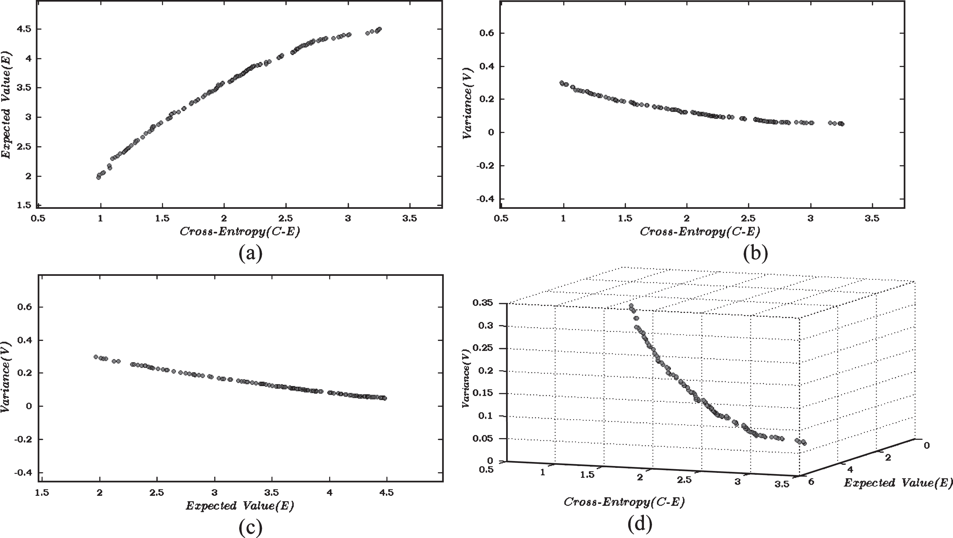
Different nondominated solutions of the proposed Portfolio model after 25000 function evaluations of NSGA-II.

Fig.2

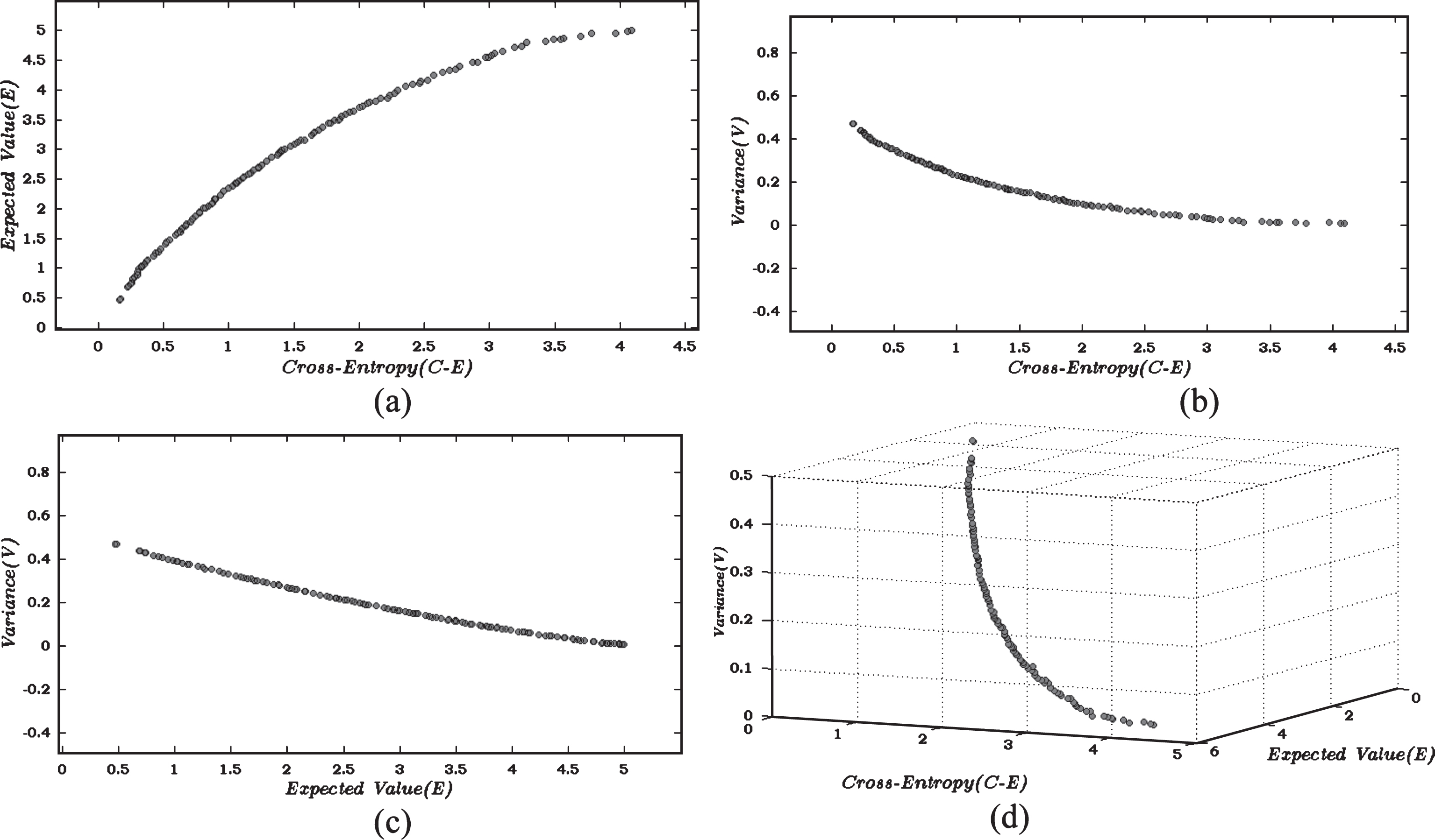
Different nondominated solutions of the proposed Portfolio model after 25000 function evaluations of AbYSS.

Nondominated solutions generated after 25,000 function evaluations, are depicted in Figs. 1(a-d) for NSGA-II and Figs. 2(a-d) for AbYSS. Figures 1(a) and 2(a) display the nondominated solutions considering two objectives, cross-entropy (D) and expected value (E). Figures 1(b) and 2(b) display the nondominated solutions for the objectives cross-entropy (D) and variance (V). Figures 1(c) and 2(c) display the nondominated solutions for expected value (E) and variance (V). Finally, Figs. 1(d) and 2(d) display the nondominated solutions considering all the 3 objectives: cross-entropy (D), expected value (E) and variance (V).

We have used jMetal 4.5 [20] framework for simulation of the MOGAs. Considering stochastic fluctuations of the MOGAs, every simulation of the results with the mentioned parameter settings as mentioned above were executed 100 times. For each execution, different performance metrics, e.g., HV [13], S [2], GD [11] and IGD [11] are evaluated for the optimized solutions obtained after 25000 function evaluations with respect to the corresponding reference front.

Different statistical measures of the performance metrics, HV, S, GD and IGD are displayed in Tables 4 and 5. Table 4 gives the mean and standard deviation (s.d.) while median and interquartile range (I.Q.R.) are shown in Table 5. The statistical parameter values in both the Tables 4 and 5 not only determine the quality of the optimized solutions obtained using two MOGAs separately but also the relative performance between them while optimizing the proposed model defined in (35).

In Table 4 we observed that AbYSS outperforms NSGA-II in terms of the performance measures, HV, S, GD and IGD for both mean and s.d. It suggests that AbYSS proves to be relatively better than NSGA-II for the proposed portfolio selection model. Table 5 shows that AbYSS is superior to NSGA-II while considering the medians for all the performance metrics. The statistical dispersion for all the performance metrics, i.e., HV, S, GD and IGD are also measured as the difference between lower and upper quartile. This measure is displayed as I.Q.R. in Table 5. By observing the I.Q.R. values of HV, GD and IGD we notice that the deviation around the median is less for AbYSS than NSGA-II. While for S, the deviation around the median is less for NSGA-II compared to AbYSS. This suggests that the probabilistic fluctuations of AbYSS after executing model (35) are less while calculating HV, GD and IGD compare to NSGA-II. In the similar way the occurrence of probabilistic fluctuation is less for S when NSGA-II is considered for execution of (35) as compared to AbYSS.

Figure 3(a-d) depict the normal probability plots of all the performance metrics. The plot includes a reference line useful for determining whether the dataset follow a normal distribution. The reference line is shown as dashed line. The performance metrics which are calculated after execution of AbYSS 100 times on model (35) are represented by ^′ × ′ symbol, where for NSGA-II the representation symbol is ^′o′ in the normal probability plots. If the dataset follows normal distribution then the elements of the dataset will concentrate around the reference line. More the elements of dataset is dispersed from the reference line there will be less chance that the dataset will follow normal distribution. From Fig. 3(a) and (b), we can affirm that, HV and S values obtained after 100 executions of AbYSS are relatively more normally distributed than those obtained by NSGA-II for same number of executions. Figure 3(c) and (d) suggest that, the values of GD and IGD obtained from 100 runs of NSGA-II are relatively more normally distributed than those which are obtained after executing AbYSS equal number of times. The affirmation related to Fig. 3(a-d) can also be verified from the p-values which are listed in Table 6. The p-values of 100 observations of HV, S, GD and IGD obtained by equal number of executions of NSGA-II and AbYSS are evaluated by conducting t-test.

Fig.3

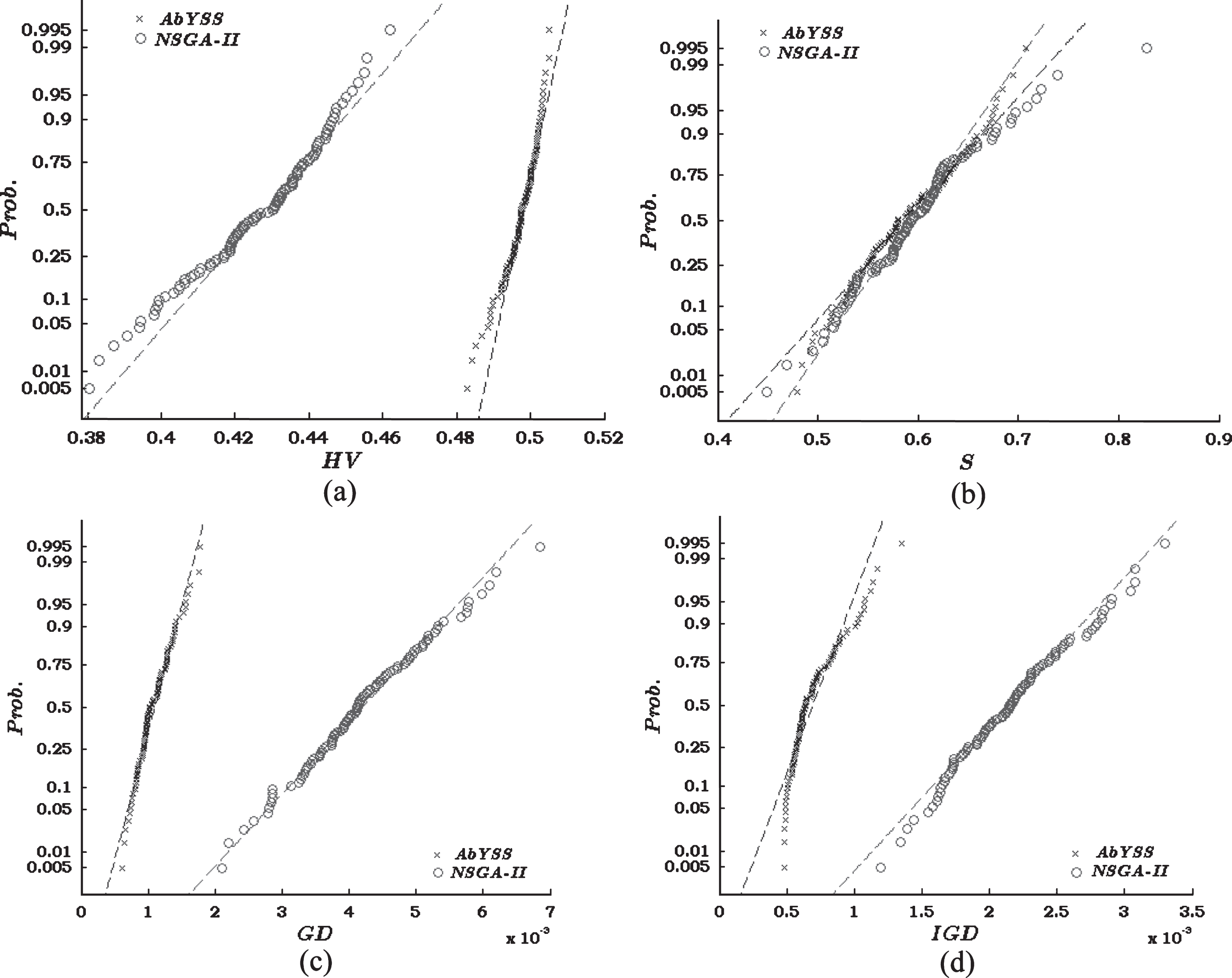
Probability plot of normal distribution for (a) HV, (b) s (c) GD and (d) IGD obtained after 100 runs of NSGA-II and AbYSS.

Table 6

p-value of different performance metrics obtained by conducting t-test

Performance	p-value of	p-value of
Metrics	AbYSS	NSGA-II
HV	6.1164e-09	1.3443e-09
S	9.2245e-08	2.3702e-08
GD	4.1154e-07	4.0793e-07
IGD	5.2429e-09	5.0138e-09

We have considered a confidence level of 95% to perform the test. For this test, we have set the null hypothesis (H₀) as the data corresponding to each dataset comes from a normal distribution. Considering AbYSS and NSGA-II, the corresponding p-values of HV and S validate our affirmation about Fig. 3(a) through Fig. 3(d), i.e., for Fig. 3(a) and (b), HV and S values obtained after execution of AbYSS [1] are more normally distributed than those obtained after executing NSGA-II [23]. Whereas, Fig. 3(c) and (d), shows that GD and IGD, obtained after execution of NSGA-II are more normally distributed than those obtained after executing AbYSS.

7 Conclusion

A multi-objective model of uncertain portfolio selection model has been proposed in this article. The model considers three objectives: maximization of expected value and minimization of both variance and cross-entropy. We have considered 20 investment returns of Shenzhen Stock Exchange for our proposed portfolio selection model. The investment returns are considered as linear uncertain variables. The proposed model is solved by two compromise multi-objective programming approaches: weighted sum approach and global criterion method. The model is also solved with two different MOGAs, namely, NSGA-II and AbYSS. The quality of solutions obtained from these MOGAs are analyzed in terms of the performance metrics HV, S, GD and IGD. We then provide some statistical interpretation on the values of those performance metrics. The overall analysis shows that AbYSS outperforms NSGA-II while solving the proposed portfolio selection model.

In future, large number of securities can be considered to study the performance of the proposed model. The proposed model can also be extended in fuzzy-random, uncertain-random and other hybrid imprecise environments.

Footnotes

Acknowledgments

The authors are very much grateful to the Editor and anonymous referees for their constructive and valuable suggestion to enhance the quality of the manuscript.

Saibal Majumder, an INSPIRE fellow (IF150410) would like to thank DST, Govt. of India, for providing him financial support for the work.

References

Nebro

A.J.

, Luna

, Alba

, Dorronsoro

, Durillo

J.J.

and Beham

, AbYSS: Adapting scatter search to multiobjective optimization, IEEE Transactions on Evolutionary Computation 12 (2008), 439–457.

Zhou

, Jin

, Zhang

, Sendho

and Tsang

, Combining model-based and genetics-based offspring generation for multiobjective optimization using a convergence criterion, in 2006 IEEE Congress on Evolutionary Computation, Sheraton Vancouver Wall Center Vancouver, BC, Canada, 2006, pp. 3234–3241.

Liu

, Theory and Practice of Uncertain Programming, 2nd edn, Springer-Verlag, Berlin, 2009.

Liu

, Uncertainty Theory, 2nd edn, Springer-Verlag, Berlin, 2007.

Liu

, Uncertainty theory: A Branch of Mathematics for Modeling Human Uncertainty, Springer-Verlag, Berlin, 2010.

Liu

, Why is there a need for uncertainty theory? Journal of Uncertain System 6 (2012), 3–10.

Liu

and Chen

X.W.

, Uncertain multiobjective programming and uncertain goal programming, Journal of Uncertainty Analysis and Applications 3 (2015), 2–8.

Coello

C.A.C.

, Evolutionary multi-objective optimization: A historical view of the field, IEEE Computational Intelligence Magazine 1 (2006), 28–36.

Feinstein

C.D.

and Thapa

M.N.

, A reformulation of a mean-absolute deviation portfolio optimization model, Management Science 39 (1993), 1552–1553.

10.

Fonseca

C.M.

and Fleming

P.J.

, Genetic algorithms for multi-objective optimization: Formulation, discussion and generalization, Proceedings of the Fifth International Conference on Genetic Algorithms, 1993, pp. 416–423.

11.

Van Veldhuizen

D.A.

and Lamont

G.B.

, Multiobjective evolutionary algorithm research: A history and analysis, Technical Report TR-98-03, Dept Elec Comput Eng, Graduate School of Eng, Air Force Inst Technol, Wright-Patterson, AFB, OH, 1998.

12.

Fishburn

D.C.

, Mean-risk analysis with risk associated with below-target returns, American Economical Review 67 (1977), 117–126.

13.

Zitzler

and Thiele

, Multi-objective evolutionary algorithms: A comparative case study and the strength Pareto approach, IEEE Transactions on Evolutionary Computation 3 (1999), 257–271.

14.

Zitzler

, Laumanns

and Thiele

, SPEA2: Improving the Strength Pareto Evolutionary Algorithm, Computer Engineering and Networks Laboratory Technical Report Department of Electrical Engineering, 2001, p. 103.

15.

Glover

, A template for scatter search and path relinking, Lecture Notes in Computer Science 1363 (1997), 13–54.

16.

Konno

and Suzuki

, A mean-variance-skewness optimization model, Journal of the Operational Research Society of Japan 38 (1995), 137–187.

17.

Konno

and Yamazaki

, Mean-absolute deviation portfolio optimization model and its applications to Tokyo stock market, Management Science 37 (1991), 519–531.

18.

Markowitz

, Portfolio selection, Journal of Finance 7(1) (1952), 77–91.

19.

Mao

J.C.T.

, Models of capital budgeting, E-V vs. E-S, Journal of Financial Quantitative Analysis 4 (1970), 657–675.

20.

Durillo

J.J.

and Nebro

A.J.

, jMetal: A Java framework for multi-objective optimization, Advances in Engineering Software 42 (2011), 760–771.

21.

Horn

, Nafploitis

and Goldberg

D.E.

, A niched Pareto genetic algorithm for multi-objective optimization, Proceedings of the First IEEE Conference on Evolutionary Computation, 1994, pp. 82–87.

22.

Knowles

and Corne

, The Pareto archived evolution strategy: A new baseline algorithm for multiobjective optimization, Proceedings of the 1999 Congress on Evolutionary Computation CEC 99, 1999, pp. 9–105.

23.

Deb

, Agrawal

, Pratap

and Meyarivan

, A fast and elitist multiobjective genetic algorithm: NSGA-II, IEEE Transactions on Evolutionary Computation 6 (2002), 182–197.

24.

Nag

, Pal

and Pal

N.R.

, ASMiGA: An archive-based steady-state micro genetic algorithm, IEEE Transactions on Cybernetics 45 (2015), 40–52.

25.

Smimou

, Bector

C.R.

and Jacoby

, Portfolio selection subject to experts’ judgments, International Review of Financial Analysis 17 (2008), 1036–1054.

26.

Yao

, A formula to calculate the variance of uncertain variable, Soft Computing 19 (2015), 2947–2953.

27.

Srinivas

and Deb

, Multiobjective function optimization using nondominated sorting genetic algorithms, Evolutionary Computation 2 (1995), 221–248.

28.

Lin

P.C.

and Ko

P.C.

, Portfolio value-at-risk forecasting with GA based extreme value theory, Expert Systems with Applications 36 (2009), 2503–2512.

29.

Jorion

P.H.

, Value at Risk: A new benchmark for measuring derivatives risk, Irwin Professional Publishers (1996).

30.

Zhang

and Li

, MOEA/D: A multi-objective evolutionary algorithm based on decomposition, IEEE Transaction on Evolutionary Computation 11 (2007), 712–731.

31.

Bhattacharyya

and Kar

, Possibilistic mean-variance-skewness portfolio selection models, International Journal of Operations Research 8 (2011), 44–56.

32.

Bhattacharyya

, Kar

and Dutta

, Majumder, Fuzzy mean-variance-skewness portfolio selection models by interval analysis, Computers and Mathematics with Applications 61 (2011), 126–137.

33.

Bhattacharyya

, Chatterjee

and Kar

, Uncertainty theory based multiple objective mean-entropy-skewness stock portfolio selection model with transaction costs, Journal of Uncertainty Analysis and Applications 1 (2013), 1–17.

34.

Yang

S.C.

, Lin

T.L.

, Chang

T.J.

and Chang

K.J.

, A semi-variance portfolio selection model for military investment assets, Expert Systems with Applications 38 (2011), 2292–2301.

35.

Rao

S.S.

, Engineering optimization: Theory and practice, 3rd edn. John Wiley & Sons, New Jersey, 1996.

36.

Rockafellar

T.R.

and Uryaser

S.P.

, Optimization of conditional value-at-risk, Journal of Risk 2 (2000), 21–41.

37.

Lai

T.Y.

, Portfolio selection with skewness: A multi-objective approach, Review of Quantitative Finance and Accounting 1 (1991), 293–305.

38.

Chen

, Kar

and Ralescu

D.A.

, Cross-entropy measure of uncertain variables, Information Sciences 201 (2012), 53–60.

39.

Huang

, Portfolio selection with fuzzy returns, Journal of Intelligent and Fuzzy Systems 18 (2007), 383–390.

40.

Huang

, Mean-entropy models for fuzzy portfolio selection, IEEE Transactions on Fuzzy Systems 16 (2008), 1096–1101.

41.

Huang

, Mean-semivariance models for fuzzy portfolio selection, Journal of Computational and Applied Mathematics 217 (2008), 1–8.

42.

Huang

, Portfolio Analysis: From probabilistic to credibilistic and uncertain approaches, Springer-Verlag, Berlin, 2010.

43.

Huang

, Mean-risk model for uncertain portfolio selection, Fuzzy Optimization and Decision Making 10 (2011), 71–89.

44.

Huang

, Mean-variance models for portfolio selection subject to expert’s estimations, Expert System with Applications 39 (2012), 5887–5893.

45.

Huang

, A risk index model for portfolio selection with return subject to expert‘s evaluations, Fuzzy Optimization and Decision Making 11 (2012), 451–463.

46.

Huang

and Qiao

, A risk index model for multi-period uncertain portfolio selection, Information Sciences 217 (2012), 108–116.

47.

Huang

and Di

, Uncertain portfolio selection with background risk, Applied Mathematics and Computation 276 (2016), 284–296.

48.

, Qin

Z.F.

and Kar

, Mean-variance-skewness model for portfolio selection with fuzzy returns, European Journal of Operational Research 202 (2010), 239–247.

49.

Gao

, Yang

, Li

and Kar

, On distribution function of the diameter in uncertain graph, Information Sciences 296 (2015), 61–74.

50.

Gao

, Yang

and Li

, Uncertain models on railway transportation planning problem, Applied Mathematical Modelling 40 (2016), 4921–4934.

51.

Sheng

and Gao

, Shortest path problem of uncertain random network, Computers & Industrial Engineering 99 (2016), 97–105.

52.

Simaan

, Estimation risk in portfolio selection: The mean variance model versus the mean absolute deviation model, Management Science 43 (1997), 1437–1446.

53.

Yoshida

, An estimation model of value-at-risk portfolio under uncertainty, Fuzzy Sets and Systems 160(22) (2009), 3250–3262.

54.

Qin

, Kar

and Li

, Developments of mean-variance model for portfolio selection in uncertain environment, Technical Report (2009).