Uncertain portfolio selection model considering transaction costs and minimum transaction lots requirement

Abstract

Due to the complexity of real security market, sometimes the future security returns can only be valued based on experts’ estimations. Meanwhile, there are transaction costs and minimum transaction lots requirement in the real transaction process in the trading market. This paper discusses the portfolio selection problem in such a circumstance. Security returns are considered as uncertain variables, and a new mean-variance model with transaction costs and minimum transaction lots is established. In addition, the impact of minimum transaction lots requirement and transaction costs on optimal portfolio is discussed and a genetic algorithm for solving the optimization model is given. As an illustration, a numerical example is provided.

Keywords

Portfolio selection mean-variance model uncertain programing genetic algorithm uncertain variable

1 Introduction

Portfolio selection is concerned with the investment of one’s money in a variety of securities so that maximum return is obtained and investment risk is controlled. Markowitz [26] first proposed the mean-variance model. In the mean-variance model, the expected return was regarded as the investment return and variance the risk. The investment strategies should be achieved on the efficient frontier of the return and risk. Since Markowitz, portfolio selection models have been put forth in extensive studies and a wealth of research results have been obtained. There are some important examples including safety-first models [19 , 37], single-factor models [33, 38], multi-factor models [8, 34], mean semi-variance models [4 , 27], expected absolute deviation methods [18, 35], Value at Risk models [17, 28], Conditional Value at Risk models [1, 36], mean semivariance-CVaR model [29], worst conditional expected value model [5], Expected Shortfall model [3], mean-risk curve model [9], etc.

In classical portfolio theory, the security returns are considered as random variables and their characteristic values such as expected value and variance are calculated based on the sample of available historical data. This calculation method implies that historical data are sufficient and can well reflect the future security returns. However, due to the complexity of the security market, historical data are sometimes insufficient or unable to reflect the future security performances. In this situation, security returns have to be given mainly by experts’ estimations rather than historical data and thus contain much subjective imprecision rather than randomness. Since men’s estimations are not random in nature and usually contain much wider range of values than the imprecise parameters really take, if we inappropriately use probability theory to deal with men’s estimations, paradoxes might appear [22]. To deal with the portfolio selection problem in this situation, Huang [10] initiated an uncertain portfolio selection theory using uncertainty theory proposed by Liu [20] as the tool. By using the uncertainty theory, no paradoxes appear. Since then many studies have been done on the development of uncertain portfolio selection theory. For example, Huang [11] further investigated the uncertain mean-variance model in depth. Huang [12] proposed a risk index model for uncertain portfolio selection, and Huang and Ying [13] further developed the model which considered portfolio adjusting problem. Li and Qin [24] studied the interval portfolio selection problem under the uncertain environment. Huang and Zhao [14] established a mean-chance model within the framework of uncertainty theory. Furthermore, Huang and Di [15] proposed and studied an uncertain portfolio model which considered not only uncertain security returns but also uncertain background assets. Qin [31] studied a portfolio selection problem in the simultaneous presence of random and uncertain returns.

In Huang’s paper [10], the transaction costs of purchasing and selling were not taken into consideration. However, there are costs such as stamp duty, transaction fees, and commissions in the procedure of purchasing and selling securities in the real life market. The transaction costs are inevitable [2]. Therefore, the ignorance of transaction costs in the model may lead to the invalid portfolio. Meanwhile, in Huang’s model [10], all securities were assumed to be infinitely divisible. Under such assumptions, the share and weight of each stock are continuous, and the corresponding efficient frontier is a continuous, uninterrupted curve. However, in the actual transaction process, each security market requires minimum transaction lots. In this case, the assumption of infinite division may result in significant error which makes it impossible for investors to achieve their target of investment, and may even bring them a loss. Therefore, it is significant to consider the minimum transaction lots in the model for practical application. The purpose of this paper is to discuss the portfolio selection problem which considers transaction costs and minimum transaction lots requirement in the uncertain environment.

The paper proceeds as follows. In Section 2, some necessary knowledge about uncertain variables will be introduced for easy understanding of the paper. In Section 3, an uncertain portfolio selection model with transaction costs and minimum transaction lots requirement in the uncertain environment will be proposed and discussed. In Section 4, the genetic algorithm will be designed for the nonlinear integer programming model we proposed. In Section 5, we will provide and discuss a numerical example to demonstrate the effectiveness of our proposed algorithm. Finally, we will conclude the paper in Section 6.

2 Necessary knowledge about uncertain variable

Necessary knowledge about the uncertainty theory used in the manuscript will be introduced in this section.

Definition 1. (Liu [20]) Let Lbe a σ-algebra over nonempty set Ω. We call every element Γ ∈ L an event. A set function M{ Γ } is called an uncertain measure if it satisfies the following four axioms:

(Normality) M { Ω } = 1;

(Self-duality) M { Γ } + M { Γ^c } = 1;

(Countable subadditivity) For each countable sequence of events {Γ_i}, We have: $M {⋃_{i = 1}^{\infty} Γ_{i}} \leq \underset{i = 1}{\sum^{\infty}} M {Γ_{i}} .$ The triplet (Ω, L, M) is called an uncertainty space.

(Product measure) (Liu [21]) For uncertainty spaces (Ω_i, L_i, M_i), i = 1, 2, …, the product uncertain measure is: $M {\underset{i = 1}{\prod^{\infty}} Γ_{i}} = \underset{i = 1}{\overset{\infty}{\land}} M {Γ_{i}}$ where Γ_i are events arbitrarily chosen from L_i for i = 1, 2, …, respectively.

Definition 2. (Liu [20]) An uncertain variable is a function η from an uncertainty space (Ω, L, M) to the set of real numbers, i.e., for any Borel set of B of real numbers, the set ${η \in B} = {χ \in Ω | η (χ) \in B},$ is an event.

Definition 3. (Liu [20]) Let η be an uncertain variable. The uncertain distribution Φ : R → [0, 1] of η is defined by $Φ (r) = M {η \leq r} .$

For example, a normal uncertain variable is the one that has the following normal uncertainty distribution $Φ (r) = {(1 + \exp (\frac{π (μ - r)}{\sqrt{3} σ}))}^{- 1}, r \in R,$ where μ and σ are real numbers and σ > 0. For the convenience of expression, we denote the normal uncertain variable by ξ ∼ N (μ, σ).

The operational law of the uncertain variables is given as follows:

Theorem 1. (Liu [23]) Let η₁, η₂, …, η_n be independent uncertain variables with continuous and strictly increasing uncertainty distribution function s Ψ₁, Ψ₂, …, Ψ_n, respectively. Let f (r₁, r₂, …, r_n) be strictly increasing with respect to r₁, r₂, …, r_n. Then $ξ = f (η_{1}, η_{2}, \dots, η_{n}),$ is an uncertain variable whose inverse uncertainty distribution function is in Equation (1): $Φ^{- 1} (γ) = f (Ψ_{1}^{- 1} (γ), Ψ_{2}^{- 1} (γ), \dots, Ψ_{n}^{- 1} (γ)),$ (1) where 0 < γ < 1.

To tell the size of an uncertain variable, Liu defined the expected value of uncertain variables.

Definition 4. (Liu [20]) Let η be an uncertain variable. Then the expected value of η is defined by $E [η] = \int_{0}^{+ \infty} M {η \geq r} dr - \int_{- \infty}^{0} M {η \geq r} dr .$

It indicates that at least one of the two integrals is finite.

Theorem 2. (Liu [23]) Let η₁ and η₂ be independent uncertain variables with finite expected values. Then for any real numbers α₁ and α₂, we have Equation (2): $E [α_{1} η_{1} + α_{2} η_{2}] = α_{1} E [η_{1}] + α_{2} E [η_{2}] .$ (2)

Definition 5. (Liu [20]) Let ξ be an uncertain variable with finite expected value e. Then the variance of ξ is defined by Equation (3). $V [ξ] = E [(ξ - e)]^{2} .$ (3)

It can be calculated that the variance value of a normal uncertain variable ξ ∼ N (μ, σ) is V [ξ] = σ².

In applications, we call $\sqrt{V [ξ]}$ standard deviation of ξ. It can be calculated that the expected value of the normal uncertain variable ξ ∼ N (μ, σ) is E [ξ] = μ, and the standard deviation of the normal uncertain variable ξ ∼ N (μ, σ) is $\sqrt{V [ξ]} = σ$ .

Theorem 3. Let ξ₁ and ξ₂ be two independent normal uncertain variables N (e₁, σ₁) and N (e₂, σ₂), respectively. Then the sum ξ₁ + ξ₂ is also a normal uncertain variable, and it can be expressed: $N (e_{1}, σ_{1}) + N (e_{2}, σ_{2}) = N (e_{1} + e_{2}, σ_{1} + σ_{2}) .$ (4)

The product of a normal uncertain variable N (e, σ) and a scalar number k is also a normal uncertain variable in Equation (5). $k \cdot N (e, σ) = N (ke, | k | σ) .$ (5)

3 Model for uncertain portfolio selection

3.1 Uncertain model

As discussed in the introduction, when security returns are given mainly by experts’ estimations, it is better to use uncertain variables to describe the security returns. Meanwhile, transaction costs and minimum transaction lots requirement usually exist in the actual transaction process in the trading market. Therefore, we take them into account in this paper.

Let ξ_i denote the uncertain returns of the ith securities which are defined as ξ_i = (p_i1 - p_i0)/p_i0, i = 1, 2, …, n, respectively, where p_i1 are the selling price of the ith securities, p_i0 are the purchasing price of the ith securities. Let a be the transaction cost rate of purchasing and b the transaction cost rate of selling. Due to transaction costs, the real yield of the security is not equal to the nominal yield. The actual expenditure of security is p_i0 (1 + a) and the actual income of the sale of security is p_i1 (1 - b). Real yield taking transaction costs into account should be as follows:

$\begin{matrix} R_{i} & = & \frac{p_{i 1} (1 - b) - p_{i 0} (1 + a)}{p_{i 0} (1 + a)} \\ = & \frac{1 - b}{1 + a} ξ_{i} - \frac{a + b}{1 + a} . \end{matrix}$ (6)

We call R_i the real yield of the ith securities.

Let q_i be the minimum transaction lots of the ith securities and x_i a positive integer which is the number of minimum transaction lots of risk asset i. It is easy to know that the transaction lots of risk security i is q_ix_i . Then the cost of purchasing risk security is q_ix_ip_i0 (1 + a). Let B be the total available funds of investors. Then the investment weight of security i is w_i = q_ix_ip_i0 (1 + a)/B. Because of the existence of minimal transaction lots requirement, it is possible that $\sum_{i = 1}^{n} w_{i}$ is not equal to 1.

Then, the return rate of the portfolio with transaction costs and minimum transaction lots requirement can be expressed as: $R_{P} = \sum_{i = 1}^{n} w_{i} (\frac{1 - b}{1 + a} ξ_{i} - \frac{a + b}{1 + a}),$ where w_i = q_ix_ip_i0 (1 + a)/B.

The expected value and the variance of the return rate of the portfolio are as follows: $E (R_{P}) = E (\sum_{i = 1}^{n} w_{i} (\frac{1 - b}{1 + a} ξ_{i} - \frac{a + b}{1 + a})),$ $V (R_{P}) = V (\sum_{i = 1}^{n} w_{i} (\frac{1 - b}{1 + a} ξ_{i} - \frac{a + b}{1 + a})),$ where w_i = q_ix_ip_i0 (1 + a)/B.

The mean-variance model aims at finding out the most desirable portfolio only by the first two moments. Expected value of the total return is regarded as the investment return, and the variance is used to measure the investment risk. A typical mean-variance model is to compromise between risk and return. For example, we may choose a portfolio with minimum investment risk on the condition that the acceptable return level is given. We may also choose a portfolio with maximum investment return on the condition that the tolerable risk level is given.

However, in practice, an alternative way is to provide a factor representing the risk preference by trading off between return and risk. Thus, we can establish the following compromise model: ${\begin{matrix} max (1 - λ) E (\sum_{i = 1}^{n} w_{i} (\frac{1 - b}{1 + a} ξ_{i} - \frac{a + b}{1 + a})) \\ - λ V (\sum_{i = 1}^{n} w_{i} (\frac{1 - b}{1 + a} ξ_{i} - \frac{a + b}{1 + a})) \\ subject to : \\ w_{i} = \frac{q_{i} x_{i} p_{io} (1 + a)}{B} \\ \sum_{i = 1}^{n} w_{i} \leq 1 \\ x_{i} \in Z, x_{i} \geq 0, i = 1, 2, \dots n . \end{matrix}$ (7)

Among them, λ ∈ [0, 1] is the risk preference coefficient. The lower the λ, the more risk preference of the investors.

3.2 Equivalent of the model

In order to solve the proposed model (7), we convert it into its equivalent when each security return rate is a normal uncertain variable.

Theorem 4. Suppose the return rates ξ_i, i = 1, 2, … n, are independent normal uncertain variables, i.e., ξ_i ∼ N (μ_i, σ_i), i = 1, 2, … n, respectively. Then model ( 7) can be converted into the following form: ${\begin{matrix} max (1 - λ) \sum_{i = 1}^{n} w_{i} (\frac{1 - b}{1 + a} μ_{i} - \frac{a + b}{1 + a}) \\ - λ {(\sum_{i = 1}^{n} (\frac{(1 - b) w_{i}}{1 + a}) σ_{i})}^{2} \\ subject to : \\ w_{i} = \frac{q_{i} x_{i} p_{io} (1 + a)}{B} \\ \sum_{i = 1}^{n} w_{i} \leq 1 \\ x_{i} \in Z, x_{i} \geq 0, i = 1, 2, \dots n . \end{matrix}$ (8)

Proof. Let $O = \underset{i = 1}{\sum^{n}} w_{i} (\frac{1 - b}{1 + a} ξ_{i} - \frac{a + b}{1 + a}) .$

As ξ_i, i = 1, 2, … n are independent normal uncertain variables, from Theorem 3, we know that O is a normal uncertain variable and $\begin{matrix} O \sim N (\underset{i = 1}{\sum^{n}} w_{i} (\frac{1 - b}{1 + a} μ_{i} - \frac{a + b}{1 + a}), \\ \underset{i = 1}{\sum^{n}} | \frac{(1 - b) w_{i}}{1 + a} | σ_{i}) . \end{matrix}$

In addition, 0 < b < 1, then $V (O) = {(\underset{i = 1}{\sum^{n}} (\frac{(1 - b) w_{i}}{1 + a}) σ_{i})}^{2},$

Thus the theorem is proved.

To consider the transaction costs and the minimum transaction lots requirement, it is necessary to analyze the impact of the minimum transaction lots requirement and transaction cost rate on the optimal value of portfolio objective function.

From model (8), it can be seen that the solving space of the problem which considers the minimum transaction lots is smaller than non-considering one. Therefore considering the minimum transaction lots will lead to the optimal value lower than the value without considering the minimum transaction lots.

Below we analyze the situation considering transaction costs. When there are no transaction costs, the model (8) is translated into the following one: ${\begin{matrix} max (1 - λ) \sum_{i = 1}^{n} {w_{i} μ_{i} - λ (\sum_{i = 1}^{n} w_{i} σ_{i})}^{2} \\ subject to : \\ w_{i} = \frac{q_{i} x_{i} p_{io}}{B} \\ \sum_{i = 1}^{n} w_{i} \leq 1 \\ x_{i} \in Z, x_{i} \geq 0, i = 1, 2, \dots n . \end{matrix}$ (9)

Although transaction costs will reduce the return of the portfolio, they also will reduce the risks of the portfolio. Theorem 5 gives the condition on which the value of optimal portfolio would diminish when considering transaction costs.

Theorem 5. Suppose the value of optimal portfolio of model (8) is ${obj}_{cost}^{*}$ , and the value of optimal portfolio of model (9) is ${obj}_{noncost}^{*}$ . For a ∈ [0, 1], b ∈ [0, 1], if $μ_{i} \leq \frac{a + b}{b (1 - b)}$ , i = 1, 2, … n, respectively, we have ${obj}_{noncost}^{*} \geq {obj}_{cost}^{*}$ .

Proof. It is clear that x_i = 0 is a feasible solution of models (8) and (9). So the optimal values of models (8) and (9) always exist and the optimal values are greater than or equal to zero.

Assume that the optimal solution of model (8) is $x_{i}^{*}$ , i = 1, 2, …, n. The value of optimal portfolio of model (8) is as follow: $\begin{matrix} {obj}_{cost}^{*} & = & \frac{1 - λ}{B} \underset{i = 1}{\sum^{n}} q_{i} x_{i}^{*} p_{i 0} ((1 - b) μ_{i} - (a + b)) \\ - \frac{λ}{B^{2}} {(\underset{i = 1}{\sum^{n}} q_{i} x_{i}^{*} p_{i 0} (1 - b) σ_{i})}^{2} \geq 0 . \end{matrix}$

If λ ≠ 0, we can get: $\frac{B (1 - λ) \underset{i = 1}{\sum^{n}} q_{i} x_{i}^{*} p_{i 0} ((1 - b) μ_{i} - (a + b))}{λ {(\underset{i = 1}{\sum^{n}} q_{i} x_{i}^{*} p_{i 0} (1 - b) σ_{i})}^{2}} \geq 1 .$

Since a ≥ 0, we have 1 + a ≥ 1. Then we can get: $\underset{i = 1}{\sum^{n}} \frac{q_{i} x_{i}^{*} p_{i 0}}{B} \leq \underset{i = 1}{\sum^{n}} \frac{q_{i} x_{i}^{*} p_{i 0} (1 + a)}{B} \leq 1,$ which means that $x_{i}^{*}$ is the feasible solution of model (9). Then we have: $\begin{matrix} {obj}_{noncost}^{*} & \geq & {obj}_{noncost} (x_{i}^{*}) \\ = & \frac{1 - λ}{B} \underset{i = 1}{\sum^{n}} q_{i} x_{i}^{*} p_{i 0} μ_{i} \\ - \frac{λ}{B^{2}} {(\underset{i = 1}{\sum^{n}} q_{i} x_{i}^{*} p_{i 0} σ_{i})}^{2} . \end{matrix}$

$\begin{matrix} {obj}_{noncost} (x_{i}^{*}) - {obj}_{cost}^{*} \\ = \frac{1 - λ}{B} \underset{i = 1}{\sum^{n}} q_{i} x_{i}^{*} p_{i 0} (b μ_{i} - a - b) \\ - \frac{λ b (1 - b)}{B^{2}} {(\underset{i = 1}{\sum^{n}} q_{i} x_{i}^{*} p_{i 0} σ_{i})}^{2} \end{matrix}$

Since $μ_{i} \leq \frac{a + b}{b (1 - b)}$ , i = 1, 2, … n, respectively, if λ ≠ 0, it is easy to know that: $\begin{matrix} \frac{B (1 - λ) \underset{i = 1}{\sum^{n}} q_{i} x_{i}^{*} p_{i 0} (b μ_{i} - a - b)}{λ b (1 - b) {(\underset{i = 1}{\sum^{n}} q_{i} x_{i}^{*} p_{i 0} σ_{i})}^{2}} \\ \geq \frac{B (1 - λ) \underset{i = 1}{\sum^{n}} q_{i} x_{i}^{*} p_{i 0} ((1 - b) μ_{i} - (a + b))}{λ {(\underset{i = 1}{\sum^{n}} q_{i} x_{i}^{*} p_{i 0} (1 - b) σ_{i})}^{2}} \\ \geq 1 . \end{matrix}$

So ${obj}_{noncost}^{*} \geq {obj}_{noncost} (x_{i}^{*}) \geq {obj}_{cost}^{*},$

if λ = 0 $\begin{matrix} {obj}_{noncost}^{*} \geq {obj}_{noncost} (x_{i}^{*}) = \frac{\underset{i = 1}{\sum^{n}} q_{i} x_{i}^{*} p_{i 0} μ_{i}}{B} \\ \geq \frac{1}{B} \underset{i = 1}{\sum^{n}} q_{i} x_{i}^{*} p_{i 0} ((1 - b) μ_{i} - (a + b)) = {obj}_{cost}^{*} . \end{matrix}$

Thus, the theorem is proved.

4 A solution algorithm

The equivalent model (8) is a complex integer nonlinear programming model and it is difficult to be solved by traditional methods. The advantage of genetic algorithm (GA) is that it can solve complex optimization problems. Based on the Darwin principle “the fittest survive” in nature, genetic algorithm (GA) was first initiated by Holland [16] and has rapidly become the best-known evolutionary techniques [7, 30]. So the GA is designed for solving the integer nonlinear programming model we proposed. The design of GA will be described below.

4.1 Chromosome representation

A feasible solution of model (8) is represented as a chromosome C = (g₁, g₂, …, g_n) where g_i, i = 1, 2, …, n represent x_i, i = 1, 2, …, n, respectively. Since the total amount of funds is fixed, then the range of values for g_i should satisfy the constraint: $\underset{i = 1}{\sum^{n}} \frac{p_{i} g_{i} q_{i 0} (1 + a)}{B} \leq 1 .$

4.2 Generate the initial population

Initialization is used to generate the first population. Define an integer pop_size as the size of the population. The procedure is described as follow:

First, generate a chromosome C = (g₁, g₂, …, g_n) randomly where for each i, g_i ∈ Z.

Second, check the feasibility of chromosome by identifying if $\sum_{i = 1}^{n} \frac{p_{i} g_{i} q_{i 0} (1 + a)}{B} \leq 1$ . If the inequality holds, the chromosome is accepted as a feasible chromosome. Then go to the third step. Otherwise, we should adjust the chromosome until it satisfies the inequality. The adjustment method is as follows:

Generate the position j randomly where g_j needs to be adjusted. To ensure the effectiveness of the adjustment process, g_j must be nonzero. Calculate the total current assets value corresponding to position j. If $p_{j} g_{j} q_{j 0} (1 + a) < \underset{i = 1}{\sum^{n}} (p_{i} g_{i} q_{i 0} (1 + a)) - B,$ let g_j = 0, and repeat the third step. Otherwise, set the g_j as follow: $g_{j} = \frac{\underset{i = 1}{\sum^{n}} (p_{i} g_{i} q_{i 0} (1 + a)) - B}{q_{j 0} p_{j} (1 + a)} .$ (10)

Third, repeat the above steps for pop_size times. Then pop_size feasible initial chromosomes are generated.

4.3 Design of the fitness function

The objective function in model (8) is a max-value function that is consistent with the largest fitness principle. Therefore, the objective function of the proposed model is taken as the fitness function. GAs require the fitness to be positive [25]. However, in our model, the objective function may be negative within the domain of definition. We should process the objective function to make it positive. The fitness function of chromosome $C_{k} = (g_{1}^{k}, g_{2}^{k}, \dots, g_{n}^{k})$ in GA is defined as: $F_{fitness} (C_{k}) = {\begin{matrix} F (C_{k}) & F (C_{k}) > 0 \\ 2 \cdot tol & F (C_{k}) = 0 \\ tol & F (C_{k}) < 0, \end{matrix}$ (11) where $\begin{matrix} F (C_{k}) & = & (1 - λ) \underset{i = 1}{\sum^{n}} p_{i} g_{i}^{k} q_{i 0} ((1 - b) μ_{i} - a - b) \\ - λ {(\underset{i = 1}{\sum^{n}} p_{i} g_{i}^{k} q_{i 0} (1 - b) σ_{i})}^{2}, \end{matrix}$ tol is an adequate small positive number, e.g. in the later example of this paper we set tol as 10^-10.

4.4 Selection operation

The roulette wheel selection method is used in the selection operation in this research. The individuals with higher fitness values are taken as parents. The elite mechanism is used to prevent the loss of high-quality individuals. The process is as follows:

First, calculate fitness value of each chromosome C_k, k = 1, 2, …, pop _ size, of the population. The maximum fitness value is F_fitness (C_max) and C_max is the corresponding chromosome.

Second, calculate propagation probability of chromosome C_k as: $P (C_{k}) = F_{fitness} (C_{k}) / \sum F_{fitness},$ (12) where P (C_k) is the probability of propagation of chromosome C_k, F_fitness (C_k) is the fitness value of chromosome C_k, ∑F_fitness is the sum of all fitness values.

Third, calculate the single cumulative probability of chromosome C_k as: $P (C_{k}) = \underset{i = 1}{\sum^{k}} P (C_{i}) .$ (13)

Fourth, generate a random number r in the from the open interval (0, 1) and then select the kth chromosome C_k if P (C_k) < r ≤ P (C_k+1).

Fifth, repeat the fourth step for pop _ size - 1 times, and combine with C_max. Then pop _ size chromosomes are selected as the parents population.

4.5 Crossover operation

The Single-point crossover operator is used to generate intersections in this research. Determine a parameter r_c ∈ (0, 1) as the probability of crossover. Pair of parents are selected for crossover in the population according to the crossover rate r_c. The crossover operator performs the exchange of segments between pair of parents [25]. The chromosome C_k is selected as a parent when the randomly generated real number r from (0, 1) is less than r_c at the kth selection, where k = 1, 2, …, pop _ size. Let $C_{1}^{'}, C_{2}^{'}, C_{3}^{'}, \dots$ denote the selected parents. The processes are as follows:

First, generate a random integer l from the open interval (0, n). Crossover operation on each pair is illustrated on $C_{1}^{'} = (L_{1}^{'}, R_{1}^{'})$ and $C_{2}^{'} = (L_{2}^{'}, R_{2}^{'})$ as follows, where $L_{1}^{'} = (g_{1}^{(1)}, g_{2}^{(1)}, \dots, g_{l}^{(1)})$ and $L_{2}^{'} = (g_{1}^{(2)}, g_{2}^{(2)}, \dots, g_{l}^{(2)})$ denote the front l numbers of genes of the chromosomes $C_{1}^{'}$ and $C_{2}^{'}$ , respectively, and $R_{1}^{'} = (g_{l + 1}^{(1)}, g_{l + 2}^{(1)}, \dots, g_{n}^{(1)})$ and $R_{1}^{'} = (g_{l + 1}^{(2)}, g_{l + 2}^{(2)}, \dots, g_{n}^{(2)})$ denote the rear n - l numbers of genes of the chromosomes $C_{1}^{'}$ and $C_{2}^{'}$ , respectively. Exchange the genes of $R_{1}^{'}$ and $R_{2}^{'}$ and produce two children as follow: $C_{1}^{″} = ({L^{'}}_{1}, {R^{'}}_{2}), C_{2}^{″} = ({L^{'}}_{2}, {R^{'}}_{1}),$ then we get two new chromosomes.

Second, as the switched new chromosome may not satisfy the constraints of the model (8). Let $C_{new}^{″} = (g_{1}^{new}, g_{2}^{new}, \dots, g_{n}^{new})$ denote the new chromosome. Check the feasibility of chromosome by identifying if $\sum_{i = 1}^{n} \frac{p_{i} g_{i}^{new} q_{i 0} (1 + a)}{B} \leq 1$ . If the inequality holds, the new chromosome is accepted as a feasible chromosome. Then go to the third step. Otherwise, we should adjust the chromosome for satisfying the inequality. The adjustment method is as follows:

Generate the position j randomly where $g_{j}^{new}$ needs to be adjusted. For ensuring the effectiveness of the adjustment process, $g_{j}^{new}$ should be nonzero. Calculate the current total assets value corresponding to the position j. If $p_{j} g_{j}^{new} q_{j 0} (1 + a) < \underset{i = 1}{\sum^{n}} (p_{i} g_{i}^{new} q_{i 0} (1 + a)) - B,$ let $g_{j}^{new} = 0$ , and repeat third step. Otherwise, set the g_j as follow: $g_{j}^{new} = \frac{\underset{i = 1}{\sum^{n}} (p_{i} g_{i}^{new} q_{i 0} (1 + a)) - B}{q_{j 0} p_{j} (1 + a)} .$ (14)

Third, repeat the above steps until all parents are crossed, then replace the parents with the feasible children.

4.6 Mutation operation

The Single point mutation operator is used in mutation operation in this research. The mutation operator performs the change of a gene of parents. Determine a parameter r_m ∈ (0, 1) as the probability of mutation. The chromosome C_k is selected as a parent when the randomly generated real number r from (0, 1) is less than r_m at the kth selection, where k = 1, 2, …, pop _ size. Let $C_{1}^{'}, C_{2}^{'}, C_{3}^{'}, \dots$ denote the selected parents. For each parent $C^{'} = (g_{1}^{'}, g_{2}^{'}, \dots, g_{n}^{'})$ , generate a random integer l from the open interval (0, n). The gene of mutation point $g_{l}^{'}$ should be generated as integer randomly in the range $[0, g_{l}^{"}]$ , where $g_{l}^{″} = \frac{B - \underset{i = 1}{\sum^{n}} (p_{i} {g^{'}}_{i} q_{i 0} (1 + a)) + p_{j} {g^{'}}_{j} q_{j 0} (1 + a)}{q_{j 0} p_{j} (1 + a)} .$ (15)

Repeat the above operation until all parents have mutation, then replace the parents with the feasible children.

4.7 Genetic algorithm

After the selection, crossover and mutation steps, the new population is ready for its next evaluation. The GA will keep running until it reaches the maximum number of iterations we specified. The process of the entire algorithm is as follows (Please also see Fig. 1):

Step 1. Generate the initial population whose size is pop _ size.

Fig.1

Flowchart of the GA in this research.

Step 2. Calculate fitness value of each chromosome in the population, and do selection process to obtain the parents population.

Step 3. Group the chromosome of parents population randomly as pairs. Generate a random number r for each pair of chromosome. If r ≤ r_c (crossover probability), then do crossover operation on the corresponding chromosome.

Step 4. Generate a random number r for each chromosome of the parent population. If r < r_m (mutation probability) then carry out mutation operation on the corresponding chromosome.

Step 5. Repeat Step 2 to Step 4 until reaching the iteration upper limit.

Step 6. Take the maximum fitness value of the chromosome as the optimal portfolio solution.

5 Numerical example

5.1 Data and calculation results

To illustrate the proposed approach for the uncertain portfolio selection with transaction costs and minimum transaction lots, we give a numerical example here. According to the experts’ estimations, the 30 risk assets’ quarterly return rates are normal uncertain variables, r_i ∼ N (μ_i, σ_i). The initial holding number of minimum transaction lots on risk assets, together with the prediction of the prices and the quarterly return rates of the 30 securities are given in Table 1.

Table 1
The prices and returns of the 30 risk assets

Risk asset i μ _i σ _i p _io Risk asset i μ _i σ _i p _io

1 0.0320 0.118 18.62 16 0.0308 0.088 22.95

2 0.0299 0.091 7.12 17 0.0324 0.114 10.23

3 0.0444 0.155 18.84 18 0.0352 0.134 17.33

4 0.0369 0.111 21.35 19 0.0390 0.142 40.40

5 0.0364 0.109 66.42 20 0.0353 0.104 12.71

6 0.0270 0.057 5.21 21 0.0346 0.096 11.19

7 0.0348 0.127 21.34 22 0.0298 0.092 33.85

8 0.0353 0.101 20.67 23 0.0312 0.091 13.66

9 0.0265 0.083 58.11 24 0.0358 0.110 9.10

10 0.0312 0.097 14.18 25 0.0416 0.144 3.27

11 0.0303 0.095 31.53 26 0.0356 0.088 4.72

12 0.0353 0.100 28.15 27 0.0259 0.079 26.55

13 0.0270 0.065 18.03 28 0.0348 0.098 32.14

14 0.0384 0.118 27.70 29 0.0320 0.110 27.40

15 0.0422 0.137 15.32 30 0.0310 0.100 15.49

Risk asset i	μ _i	σ _i	p _io	Risk asset i	μ _i	σ _i	p _io
1	0.0320	0.118	18.62	16	0.0308	0.088	22.95
2	0.0299	0.091	7.12	17	0.0324	0.114	10.23
3	0.0444	0.155	18.84	18	0.0352	0.134	17.33
4	0.0369	0.111	21.35	19	0.0390	0.142	40.40
5	0.0364	0.109	66.42	20	0.0353	0.104	12.71
6	0.0270	0.057	5.21	21	0.0346	0.096	11.19
7	0.0348	0.127	21.34	22	0.0298	0.092	33.85
8	0.0353	0.101	20.67	23	0.0312	0.091	13.66
9	0.0265	0.083	58.11	24	0.0358	0.110	9.10
10	0.0312	0.097	14.18	25	0.0416	0.144	3.27
11	0.0303	0.095	31.53	26	0.0356	0.088	4.72
12	0.0353	0.100	28.15	27	0.0259	0.079	26.55
13	0.0270	0.065	18.03	28	0.0348	0.098	32.14
14	0.0384	0.118	27.70	29	0.0320	0.110	27.40
15	0.0422	0.137	15.32	30	0.0310	0.100	15.49

According to the requirements of Chinese securities market, for each risk asset, the minimum transaction lots is 100 shares. That means the investor must hold multiples of 100 shares of each risk asset. The cost transaction rate of purchasing is 0.08%, and the cost transaction rate of selling is 0.1%. The risk preference coefficient of investors is 0.3, and the total investment capital is 1,000,000.

Then a practical experiment is implemented. Parameters are placed according to the complexity of the problem: pop _ size is 100, the number of cycles is 2000, r_c is 0.7 and r_m is 0.1. The calculation is conducted with Matlab R2013a on the Intel Core i3-3120M processor with 2.50 GHz RAM. Computation time of the example is 3.601 seconds. The result converged and stabled after 1300 cycles. The procedure of convergence is shown in Fig. 2.

Fig.2

The procedure of convergence.

We get the optimal combination of risk assets as follows $x (i) = {\begin{matrix} 157 & i = 3 \\ 459 & i = 15 \\ 0 & other . \end{matrix}$ (16)

The maximum expected return rate is 4.09%, and the corresponding risk level is 1.97%. The maximum fitness value is 0.0226, the funds invested in the portfolio is 999966.1263.

To verify the robustness of GA, ten tests were taken. The results are shown in the following table. As we can see in Table 2, the optimal results verified little during ten repeated tests. So the algorithm is believed to be robust.

Table 2

The optimal values the 10 experiment

	Test 1	Test 2	Test 3	Test 4	Test 5
Return rate	4.09%	4.06%	4.09%	4.12%	4.10%
Risk level	1.97%	1.90%	1.98%	2.01%	2.02%
Fitness value	0.0226	0.0223	0.0226	0.0229	0.0227
	Test 6	Test 7	Test 8	Test 9	Test 10
Return rate	4.06%	4.07%	4.11%	4.07%	4.11%
Risk level	1.87%	1.93%	1.99%	1.95%	2.01%
Fitness value	0.0222	0.0223	0.0227	0.0224	0.0227

Model (8) includes the risk preference coefficient λ, the transaction costs of purchasing a and the transaction costs of selling b. We analyze the impact of these factors on the portfolio through simulation.

5.2 Impact of the risk preference coefficient λ on the portfolio

Figure 3 shows the impact of the risk preference coefficient λ on the gain of investment portfolio, Fig. 4 shows the result of influence of the risk preference coefficient λ on the risk of investment portfolio, and Fig. 5 shows the impact of the λ on portfolio objectives.

Fig.3

Impact of λ on the benefit.

Fig.4

Impact of λ on the risk.

Fig.5

Impact of λ on the objective function.

It can be seen from Figs. 3–5 that when λ is zero; the investor prefers to fully accept the risk. Thus, the penalty term in corresponding objective function is not binding to investors. In this case, investors only focus on the pursuit of maximum benefit. The target is equal to investment income, and all funds are put into the third asset which has the largest income. As the risk preference coefficient λ increases, the penalty term in the objective function is beginning to take effect that it lead to the value of the objective function reduced. When λ is small, the influence of penalty term is not obvious, therefore portfolio earnings are not affected. When it comes to 0.2, the revenue becomes insufficient to cover the risk caused by penalty term in the objective function, and the investors have to change investment strategy and choose less risky assets investment. When this happens, because of the low income of less risk assets, the optimal of both earnings and portfolio objective function value will reduce. When λ reaches up to 1, investors will not accept the risk at all and they will not invest in any assets.

5.3 Impact of the transaction costs of purchasing a and the transaction costs of selling b on investment portfolio

This section studies the influence exerted by a and b. The optimal values with different transaction rates are shown in Table 2. In this numerical example, there are $μ_{i} \leq \frac{a + b}{b (1 - b)}$ , i = 1, 2, … n, respectively, that is to say, according to Theorem 5, the optimal value without transaction rates is greater than it is with transaction rates. This can be verified in Table 3.

Table 3
The optimal values with a and b

a 0 0.0002 0.0005 0.0007 0.001

b

0 0.02386 0.02371 0.02350 0.02335 0.02313

0.0002 0.02372 0.02357 0.02335 0.02320 0.02298

0.0005 0.02350 0.02335 0.02313 0.02299 0.02277

0.0007 0.02335 0.02320 0.02299 0.02284 0.02262

0.001 0.02313 0.02299 0.02277 0.02262 0.02240

a	0	0.0002	0.0005	0.0007	0.001
b
0	0.02386	0.02371	0.02350	0.02335	0.02313
0.0002	0.02372	0.02357	0.02335	0.02320	0.02298
0.0005	0.02350	0.02335	0.02313	0.02299	0.02277
0.0007	0.02335	0.02320	0.02299	0.02284	0.02262
0.001	0.02313	0.02299	0.02277	0.02262	0.02240

Figure 6 shows the impact of a on the optimal value of investment portfolio. Figure 7 shows the impact of b on the optimal value. The axis y indicates the optimal value. It can be inferred that the transaction costs lead to decrease of the objective and the larger the transaction costs, the lower the optimal fitness value would be.

Fig.6

Impact of transaction cost rate a on benefit.

Fig.7

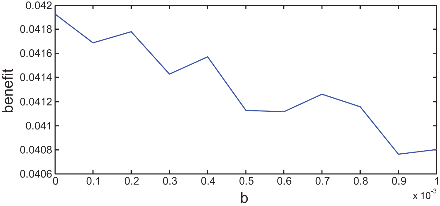
Impact of transaction cost rate b on benefit.

Figure 8 shows the impact of a on the risk of investment portfolio, and Fig. 9 shows the impact of b on risk. These graphs reveal that the effect of transaction costs rate of purchasing a and transaction costs rate of selling b mainly focus on the earning. The greater the transaction costs, the lower benefit of the portfolio. Meanwhile, these graphs reveal that both a or b have little effect on the risk. The transition costs have little influence over the investment risks.

Fig.8

Impact of transaction cost rate a on risk.

Fig.9

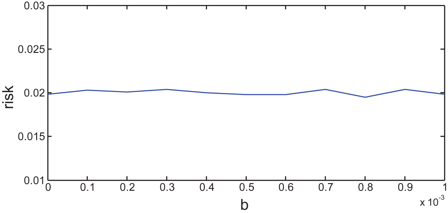
Impact of transaction cost rate b on risk.

5.4 Summary

The risk preference coefficient λ represents investors’ preference level for risk. As λ increases, the investors’ willingness of taking risk is dropping. Investors are reluctant to invest in risk assets. Generally speaking, the less risk assets the less earnings, therefore the optimal value of gains and portfolio objective function decrease with increase of the risk preference coefficient λ.

Transaction cost rate has an effect on the benefit of portfolio. And the larger the transaction rates, the lower the investment portfolio benefit. In contrast, the transaction cost rate of selling has greater effect on portfolio return than on the purchasing. Transaction cost rate has little impact on risks.

6 Conclusions

This paper has discussed the portfolio selection problem which considers transaction costs and minimum transaction lots requirement in the uncertain environment where security returns are given by experts’ estimations rather than historical data. Uncertain variables are used to describe the security returns. A new mean-variance model has been given. The impact of minimum transaction lots requirement and transaction costs on optimal portfolio has been discussed and a genetic algorithm for solving the optimization model has been provided. A numerical experiment has been given to illustrate the application of the proposed model and check the efficiency and robustness of the proposed algorithm. The computational results indicate that the proposed model is meaningful and able to be applied in reality.

References

Artzner

, Delbaen

, Eber

and Heath

, Thinking coherently, Risk 10 (1997), 68–71.

Arnott

R.D.

and Wagner

W.H.

, The measurement and control of trading costs, Finan Anal J 6 (1990), 73–80.

Adam

, Houkari

and Laurent

J.P.

, Spectral risk measures and portfolio selection, J Bank Financ 32 (2008), 1870–1882.

Ballestero

, Mean-semivariance efficient frontier: A Downside risk model for portfolio selection, App Math Financ 12 (2005), 1–15.

Benati

, The optimal portfolio problem with coherent risk measure constraints, Eur J Oper Res 150 (2003), 572–584.

Grootveld

and Hallerbach

, Variance vs downside risk: Is there really that much difference? Eur J Oper Res 114 (1999), 304–319.

Goldberg

D.E.

, Genetic Algorithms in Search Optimization, and Machine Learning. Ed. Boston: Addison- Wesley, 1989.

Giove

, Funari

and Nardelli

, An interval portfolio selection problem based on regret function, Eur J Oper Res 170 (2006), 253–264.

Huang

X.X.

, Portfolio selection with a new definition of risk, Eur J Oper Res 186 (2008), 351–357.

10.

Huang

X.X.

, Portfolio Analysis: From Probabilistic to Credibilistic and Uncertain Approaches, Ed. Berlin: Springer-Verlag, 2010.

11.

Huang

X.X.

, Mean-variance models for portfolio selection subject to experts’ estimations, Expert Syst Appl 39 (2012), 5887–5893.

12.

Huang

X.X.

, A risk index model for portfolio selection with returns subject to experts’ estimations, Fuzzy Opt Dec Mak 11 (2012), 451–463.

13.

Huang

X.X.

and Ying

H.Y.

, Risk index based models for portfolio adjusting problem with returns subject to experts’ evaluations, Econ Modelling 30 (2013), 61–66.

14.

Huang

X.X.

and Zhao

T.Y.

, Mean-chance model for portfolio selection based on uncertain measure, Insur Math Econ 59 (2014), 243–250.

15.

Huang

X.X.

and Di

, Uncertain portfolio selection with background risk, Appl Math Comput 276 (2016), 284–296.

16.

Holland

J.H.

, Adaptation in natural and artificial systems: An introductory analysis with applications to biology, control, and artificial intelligence, University of Michigan Press, Ann Arbor, 1975.

17.

Jorion

, Measuring the risk in value at risk, Financ Anal J 52 (1996), 47–56.

18.

Konno

and Yamazaki

, Mean-absolute deviation portfolio optimization model and its application to Tokyo stock market, Manag Sci 37 (1991), 519–531.

19.

Kataokas

, A Stochastic programming model, Econometrica 31 (1963), 181–196.

20.

Liu

, Uncertainty Theory, second ed, Springer-Verlag, Berlin, 2007.

21.

Liu

, Some research problems in uncertainty theory, J Uncertain Syst 3 (2009), 3–10.

22.

Liu

, Why is there a need for uncertainty theory? J Uncertain Syst 6 (2012), 3–10.

23.

Liu

, Uncertainty theory: A Branch of Mathematics for Modeling Human Uncertainty, Springer-verlag, Berlin, 2010.

24.

and Qin

Z.F.

, Interval portfolio selection models within the framework of uncertain theory, Econ Modelling 41 (2014), 338–344.

25.

Michalewicz

, Genetic algorithms + Data structures = Evolution programs, Springer, Heidelberg, 1996.

26.

Markowitz

, Portfolio selection, J Financ 7 (1952), 77–91.

27.

Markowitz

, Portfolio Selection: Efficient Diversification of investments, Wiley, New York, 1959.

28.

Natasa

, Miles

and Andrea

, Var optimal portfolio with transaction costs, Appl Math Comput 218 (2011), 4624–4637.

29.

Najafi

A.A.

and Mushakhian

, Multi-stage stochastic mean-semivariance-CVaR portfolio optimization under transaction costs, Appl Math Comput 256 (2015), 445–458.

30.

Park

Y.B.

, Yoo

J.S.

and Park

H.S.

, A genetic algorithm for the vendor-managed inventory routing problem with lost sales, Expert Syst Appl 53 (2016), 149–159.

31.

Qin

Z.F.

, Mean-variance model for portfolio optimization problem in the simultaneous presence of random and uncertain returns, Eur J Oper Res 245 (2015), 480–488.

32.

Roy

A.D.

, Safety-first and the holding of assets, Econometrica 20 (1952), 431–449.

33.

Ross

S.A.

, The arbitrage theory of capital asset pricing, J Econ Theory 13 (1976), 341–360.

34.

Sharpe

W.F.

, A simplified model for portfolio analysis, Manag Sci 9 (1963), 277–293.

35.

Simaan

, Estimation risk in portfolio selection: The mean-variance model and the mean-absolute deviation model, Manag Sci 43 (1997), 1437–1446.

36.

Tong

X.J.

, Qi

L.Q.

, Wu

and Zhou

, A smoothing method for solving portfolio optimization with CVaR and applications in allocation of generation asset, Appl Math Comput 216 (2010), 1723–1740.

37.

Telser

L.G.

, Safety first and hedging, Rev Econom Studies 23 (1956), 1–16.

38.

Xia

Y.S.

, Liu

B.D.

, Wang

S.Y.

and Lai

K.K.

, A model for portfolio selection with order of expected returns, Comput Oper Res (2000), 27409–422.