Optimization of artificial CNN based on swarm intelligence algorithm

Abstract

Aiming at the precocious convergence, low search accuracy and easy divergence of most particle swarm optimizations with velocity terms, a particle swarm optimization (IWPSO) with random inertia weights and quantization is proposed. First, the inertia weights are obeyed to be distributed randomly, and the learning factors are adjusted asynchronously to optimize the parameters in BP network. Secondly, BP network is trained using the IWPSO algorithm based on the sample data. Finally, simulation experiments prove that the algorithm has significantly improved search speed, convergence accuracy, and stability compared with existing improved algorithms. Due to the characteristics of IWPSO algorithm, the BP neural network optimized by IWPSO has better global convergence performance and is an efficient particle swarm optimization.

Keywords

Optimization artificial neural network swarm intelligence algorithm

1 Introduction

As a kind of advanced artificial intelligence technology, artificial neural network is very suitable for processing non-linear and noisy data, especially for those problems that are characterized by fuzzy, incomplete and inadequate knowledge or data [1, 2]. Ann is an information processing system constructed by imitating the structure and function of brain neurons in biology, using physical, mathematical, statistical, computer science and engineering methods to study the intelligent behavior of human beings and simulate the information processing function of human brain. Building a kind of intelligent machine that can realize human intelligent activities and develop intelligent application technology. Artificial neural network has been widely used to solve problems such as pattern recognition, prediction, optimal control and intelligent decision-making [3, 4]. Artificial neural network is one of the major and hot scientific research fields that human beings are facing. Among them, BP neural network has the most extensive research and application [5].

Rumelhart and McCelland proposed BP neural network in 1986 [6, 7]. Therefore, BP neural network is the most widely studied and applied among artificial neural networks [8, 9]. Many experts and scholars have put a lot of energy into research on these BP neural network problems [10 –14]. Hao et al. [15] fully considered the search results in the completed iterations to determine the selection of the learning rate η and the momentum moment a during the weight training of the BP network. Therefore, it can better avoid falling into local minima and have a faster training speed. Liang et al. [16] proposed an adaptive learning rate factor to improve the BP algorithm and use it in the learning of two-dimensional XOR problems and multi-dimensional XOR problems. Liu et al. [17] proposed an improved variable learning rate BP algorithm to solve problems such as slow convergence and fixed learning rate in BP neural networks. Heravi et al. [18] proposed a blind equalization algorithm capable of adaptively adjusting the momentum to eliminate inter-symbol crosstalk generated during digital signal transmission. Tang et al. [19] established for corporate credit analysis, rating and judgment with an adaptive learning rate. Saffaran et al. [20] proposed a algorithm combining traditional BP algorithm. Yao [21] used the neural network to solve the inherent defects of BP neural network in analog circuit fault diagnosis. Xu et al. [22] optimized the BP neural network. Liu et al. [23] used genetic algorithm to optimize BP network. Nagra et al. [24] proposed an algorithm by an adaptive particle swarm that dynamically changes inertia weight. Li et al. [25] introduced random inertia weights to the inherent basic particle swarm algorithm to improve the PSO algorithm, overcoming the problems of slow convergence and low accuracy in the later stages of the basic PSO algorithm. Zeng et al. [26] simplified the structure of the standard particle swarm optimization. Harrison et al. [27] proposed an adaptive extended simplified particle swarm optimization and to get rid of the problem of the algorithm being trapped in a local optimum. Wang et al. [28] proposed a method combining quantum computing and particle swarm optimization to solve the problem of multiprocessor height. This method not only has fast optimization, but also improves the convergence accuracy of the late evolutionary algorithm. Chen et al. [29] introduced genetic operator mechanism to the design of particle swarm algorithm, and established algorithm based on genetic operator. Lalwani et al. [30] used a BP network-learning algorithm by using mutated particle swarm optimization (MPSO) for intrusion detection. Li et al. [31] applied the BP network based on adaptive particle swarm algorithm (AMPSO) to network intrusion data detection, and proved the superiority and practicability. Qiao et al. [32] proposed a learning algorithm (MBPPSO) for graduate admission and employment prediction problems.

Although BP neural network algorithm is a supervised learning algorithm, the BP neural network algorithm still has the following shortcomings in practical application [33]. We propose a quantized particle swarm optimization (IWPSO) algorithm with stochastic inertial weight. The algorithm optimizes the parameters in BP neural network by means of inertia weight obeying random distribution and learning factor changing asynchronously.

2 BP network

2.1 Principle of BP network

The principle of BP network trains network according to the algorithm of error inverse propagation. There are three layers: input layer, hidden layer and output layer [34].

From Fig. 1, the information is sent from the output layer, arrives at the hidden layer, and is converted into another signal by the processing of the transfer function and is output by the output layer. Finally, if the output layer in the process of training the output result is not ideal, the back propagation error to iterate through cumulative value and threshold value, until the network output value is more close to the actual output value did not stop training.

Fig.1

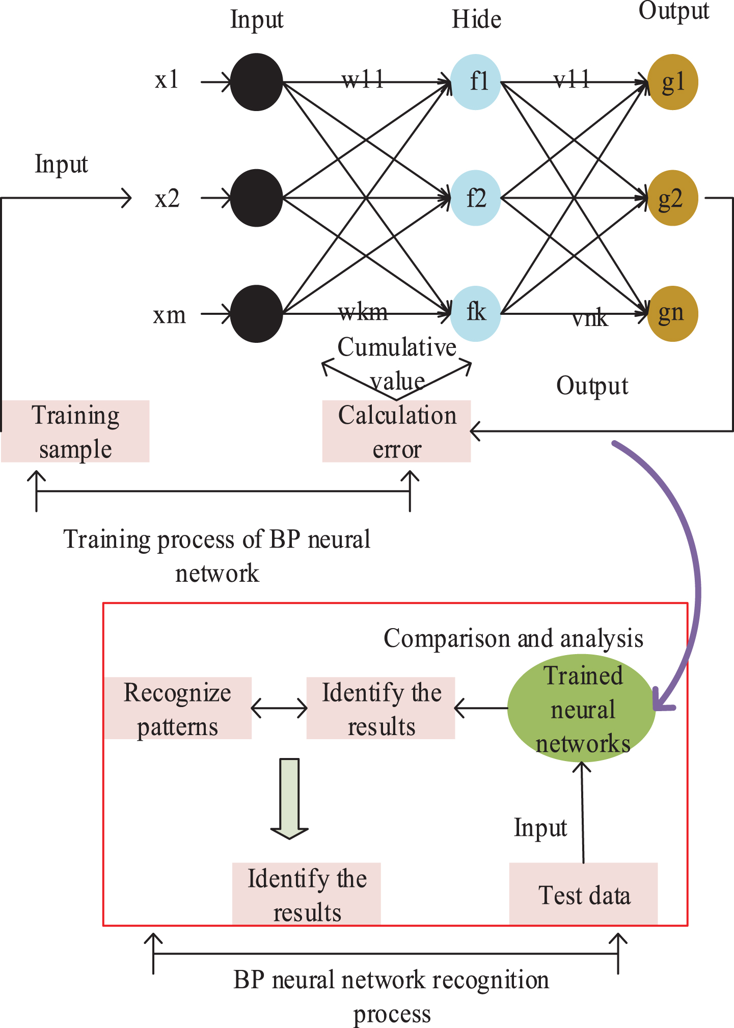
Application structure diagram of BP neural network model.

2.2 Algorithm flow of BP network

BP is a typical supervised learning method. The training process is characterized by self-learning habit and self-organization, and it can obtain ideal output expectation through training. The learning algorithm steps of BP neural network are as follows [35].

Step 1: Determine input sample and corresponding expectations

If the input sample in-group k is x_k = x_1k, x_2k, . . . , x_nk, there must be a corresponding output sample y_k = y_1k, y_2k, . . . , y_mk.

Step 2: Calculate the actual output and target function:

According to the transfer function of the network: $y_{i} = \frac{1}{1 + e^{(- \sum w_{ij} x_{i})^{- 1}}}$ (1)

Step 3: When the learning sample passes and reaches the output network, an objective is needed to determine whether the error of the output value is within the allowable error range. Where, the error value is e_k: $e_{k} (t) = \frac{1}{2} \sum_{m} {[t_{mk} - o_{mk} (t)]}^{2}$ (2)

Where, m in formula (2) represents the output layer neuron, and o_mk (t) represents the output value. Objective of the total evaluation of the network is shown in formula (3). $E (t) = \sum_{k} e_{k} (t)$ (3)

Step 4: Back propagation calculation.

Adjust the weight layer by layer until the network error is within the allowable error range. $w_{ij} (t + 1) = w_{ij} (t) + Δ w_{ij} (t) = w_{ij} (t) - η \sum_{k} \frac{\partial E_{k} (t)}{\partial w_{ij} (t)}$ (4)

(1) If i is the output neuron, then i = m, then $\frac{\partial E_{k} (t)}{\partial w_{ij} (t)} = - | t_{mk} - o_{mk} (t) | f (x_{mk}) I_{jk}$ (5)

In the formula, I_jk indicates that when the sample k is passed to the node as the input value of the i node, the original function is: $f (x) = \frac{1}{1 + e^{- x}}$ (6)

(2) If i is not the output neuron, then $\frac{\partial E_{k}}{\partial w_{ij}} = f (x_{ik}) I_{jk} \sum_{z} δ_{zk} w_{zj}$ (7)

Step 5: Go back to step 3 and stop training until the network training error is within the allowable error range. The specific process is shown in Fig. 2.

Fig.2

BP neural network algorithm flowchart.

2.3 Defects and shortcomings of BP network

Application of BP is spread, and has been applied in many practical applications, but many problems have also been found in the practical application process [36 –39].

The learning efficiency is relatively low and the convergence rate is slow [40]. In recent years, with the development of computer technology, some complex optimization problems that could not be solved in the past can be solved by computer to obtain approximate solutions. Therefore, it is more and more important to study the methods of solving optimization problems by computer.

Method for computer to solve the optimization problem is to search the feasible solution space of the optimization problem [41, 42]. In the years, foreigners have begun to study swarm intelligence algorithms. Random method is an effective solution to the problem of global optimization method of universal adaptability, especially inspired by biological evolution and genetics theory of evolutionary algorithms (genetic algorithm), due to the strong generality, analytical nature almost no requirements for the objective function, has become the main methods to solve complex optimization problems.

The basic idea of this kind of algorithms is to simulate the swarm behavior of natural organisms to construct random optimization algorithms [43]. The so-called group intelligence refers to the behavior of individuals in a group learning from each other and competing with each other.

3 BP neural network optimization based on PSO

3.1 Basic PSO

Particle Swarm Optimization (PSO) is an intelligent optimization algorithm. The principle is to compare the search space of our problem to the flight space of a bird.

The vectors of the position is x_i = x_i1, x_i2, . . . , x_id and velocity is v_k = v_i1, v_i2, . . . , v_id. And its update formula is shown in formula (8) and formula (9). $v_{ij} (t + 1) = {wv}_{ij} (t) + c_{1} r_{1} [p_{ij} - x_{ij} (t)] + c_{2} r_{2} [p_{ij} - x_{ij} (t)]$ (8) $x_{ij} (t + 1) = x_{ij} (t) + v_{ij} (t + 1)$ (9)

Among them, the optimal position of each individual for each particle is denoted as pbest, and the optimal position of all particles in the overall optimization process is denoted as gbest.

After induction and summary, the basic process of a single PSO is obtained from Fig. 3.

Fig.3

PSO algorithm flowchart.

3.2 Particle swarm optimization

The state of particles is described by the wave function ψ (x, t). By solving the Schrodinger equation, the probability density function of a particle at a certain point in space is obtained. Then, the position equation of the particle is obtained by random simulation: $x (t) = P \pm L ln (1 / u) / 2$ (10)

The variable u varies in the range [0, 1], and L is defined as: $L (t + 1) = 2 β * | mbest - x (t) |$ (11) $mbest = \sum_{i = 1}^{M} \frac{P_{i}}{M} = (\sum_{i = 1}^{M} \frac{P_{i 1}}{M}, \sum_{i = 1}^{M} \frac{P_{i 2}}{M}, . . ., \sum_{i = 1}^{M} \frac{P_{iD}}{M})$ (12)

Finally, the position of the particle is: $x (t + 1) = P \pm β * | mbest - x (t) | ln (1 / u)$ (13)

To avoid problems of divergence of particles with velocity vectors, slow convergence and low accuracy in the later period, the PS0 formula with quantum behavior is simplified to remove the particle velocity term. Only the position vector controls the search process. The specific optimization algorithm four-update formulas are as follows: $x_{id}^{t + 1} = {wx}_{id}^{t} + c_{1} r_{1} [{pbest}_{id} - x_{id}^{t}] + c_{2} r_{2} [{gbest}_{id} - x_{id}^{t}]$ (14)

Among them, t is current iteration times. The variable w is weight. Variable c1 is an influencing factor of an individual’s “self-awareness” ability. The variable c2 is an influencing factor of an individual’s “social cognition” ability. pbest_id is the individual optimal, and gbest_id is the global optimal.

3.3 Optimization of random inertia weights

According to the characteristics of the PSO algorithm, it can be known that when the weight is set large, so that current optimal solution space can be searched quickly. However, when the weight is set to a small value, its local optimization capability is very strong, and the convergence speed is fast. As shown in Fig. 4, it shows the connection between the weight change and convergence.

Fig.4

Relation between weight change and convergence.

It can be seen from Fig. 4 that the change of max [||α||, ||β||] decreases first and then increases, and the critical value of the weight is one. When the weight is less than one, the particle swarm algorithm is in a state of convergence. When the weight is 0.2, max [||α||, ||β||] reaches the minimum value. Therefore, the convergence speed is the fastest at this time. However, as the weights continue to increase, the convergence rate continues to slow down. When the weights are greater than one, the particle swarm algorithm no longer converges. Therefore, value range of weight is required to be [0.2, 1.4].

The inertia weight is a random number that follows a certain distribution. By using the uncertain property of random variable to adjust the inertia weight, the algorithm can jump out of the local optimal quickly. It is beneficial to maintain the diversity of the population and improve the global search performance of the algorithm. Because of the randomness, the particle has the chance to get a large or small weight value in the initial stage of operation and a small or large weight value in the later stage of calculation. If the particle is near the optimal particle, the weight of inertia of random distribution can produce a relatively small value. This is beneficial to meet the requirements of refined search, avoid flying over the optimal solution space, and accelerate the convergence speed of the algorithm. If the random inertia weight is a larger value, the larger value will be obtained when the adaptive function is calculated, and its value is less than the optimal value. In this case, the larger inertia weight will be eliminated. The algorithm will regenerate the new weight of inertia. If the particle is far away from the optimal particle, the random inertia weight has a chance to produce a larger value. In this way, the global search of particles can be satisfied and the local optimum and prematurity can be avoided, and the convergence speed of the algorithm can also be accelerated. If the value of the random inertia weight is small, the value of the adaptive function obtained will be worse than the optimal one. The smaller inertia weight will also be eliminated, and the inertial weight value of the algorithm will be generated again. Moreover, the method of random distribution is used to generate the weight value. The algorithm can get a better weight value in the later stage, and the adaptive function value stagnation phenomenon will not occur in the algorithm. Therefore, the formula for the random inertia weight w is as follows: $w = μ_{min} + (μ_{max} - μ_{min}) rand () + σ rand ()$ (15)

Among them, μ_min is minimum value of the average value, μ_max is maximum value of the average value of the random inertia weight. Influence degree of uniform distribution in the weight w is restricted by μ_max - μ_min.

3.4 Asynchronous learning factors

In the standard PSO algorithm, learning factor c1 controls individuals’ “self-cognition” ability, while learning factor c2 controls individuals’ “social cognition” ability. The two learning factors adopt different change strategies in the optimization process, which are called asynchronous change learning factors. Factor c1 is taken as a larger value to make particles learn more from themselves and less from the society. Factor c2 value is larger, so that the particles learn more from the social optimal and less from their own optimal, which is conducive to convergence. Following formula for the change of learning factors is proposed: $c_{1} = c_{1 ini} - (c_{1 ini} - c_{1 fin}) (t / T_{max})$ (16) $c_{2} = c_{2 ini} + (c_{2 fin} - c_{2 ini}) (t / T_{max})$ (17)

Where, variable c_1ini and variable c_2ini respectively represent the initial values of learning factors, c_1fin and c_2fin respectively represent iteration end values of learning factors c1 and c2, represent the current iteration times, and T_max represents the maximum iteration times.

3.5 Parameter optimization of BP based on IWPSO

When using the IWPSO to train a BP network, all parameters should first be encoded as individuals represented by real digital strings. Assuming that the network contains M optimization parameters, each individual will be an M-dimensional vector composed of M parameters to represent.

The components of each individual in the particle swarm are mapped to the parameters of the network to form a BP neural network. For each neural network corresponding to each individual, input training samples for training. The mean square error of each network on the training set is calculated: $E (x_{p}) = \frac{1}{2 n} \sum_{p = 1}^{n} \sum_{k = 0}^{c} [y_{kp} (x_{p}) - d_{kp}]^{2}$ (18)

Where y_kp the actual network is output of the training sample p at the output of k, and d _ kp is the corresponding given output. The specific process is shown in Fig. 5.

Fig.5

Flow chart of quantized particle swarm optimization based on random inertia weights.

4 Experiments and results

4.1 Fitting effect and accuracy analysis of un-optimized BP network

Training model used is a single BP network. Parameters of the network are given in Table 1 below.

Table 1
BP neural network training parameters

Training times Training goal Learning rate

500 0.0001 0.01

Training times	Training goal	Learning rate
500	0.0001	0.01

Figure 6 shows the BP neural network training process diagram, which shows the fitness function value of the network model and the number of network training times.

Fig.6

The training process diagram of BP neural network.

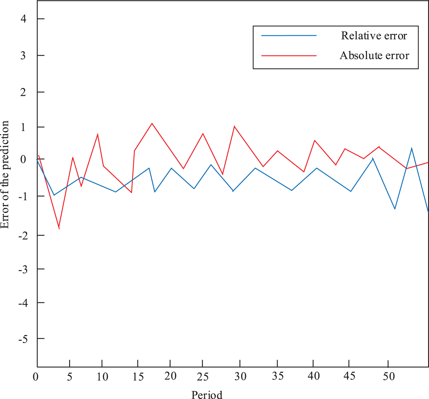
Figure 7 shows the fitting effect. Figure 8 shows absolute error and relative error in fitting accuracy. From Fig. 7 that fitting effect of a single BP is not very good. Figure 8 can find that prediction accuracy of the BP is also unsatisfactory. The main reason is that when a single BP neural network optimizes a complex function with multiple minima. In the training process, it is easy to fall into the local minimum, which cannot be escaped in this direction, resulting in poor search results.

Fig.7

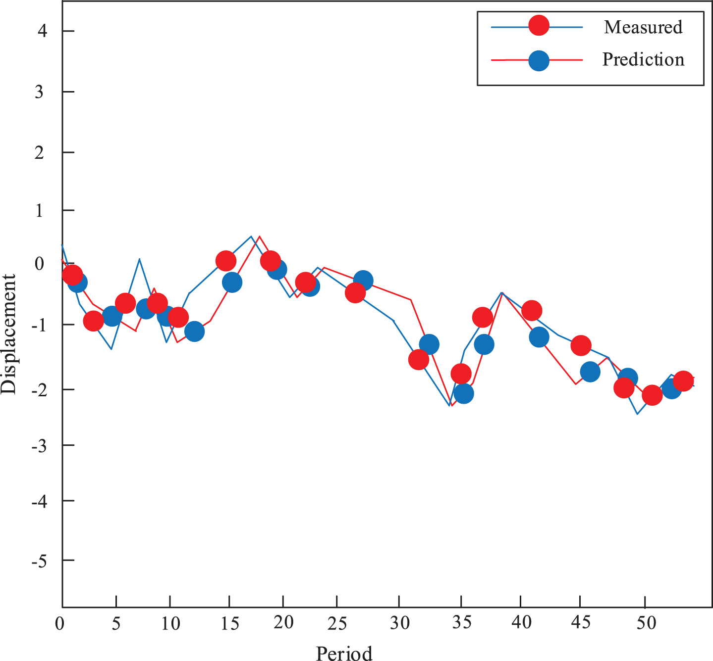
Fitting effect of the prediction algorithm of the BP algorithm.

Fig.8

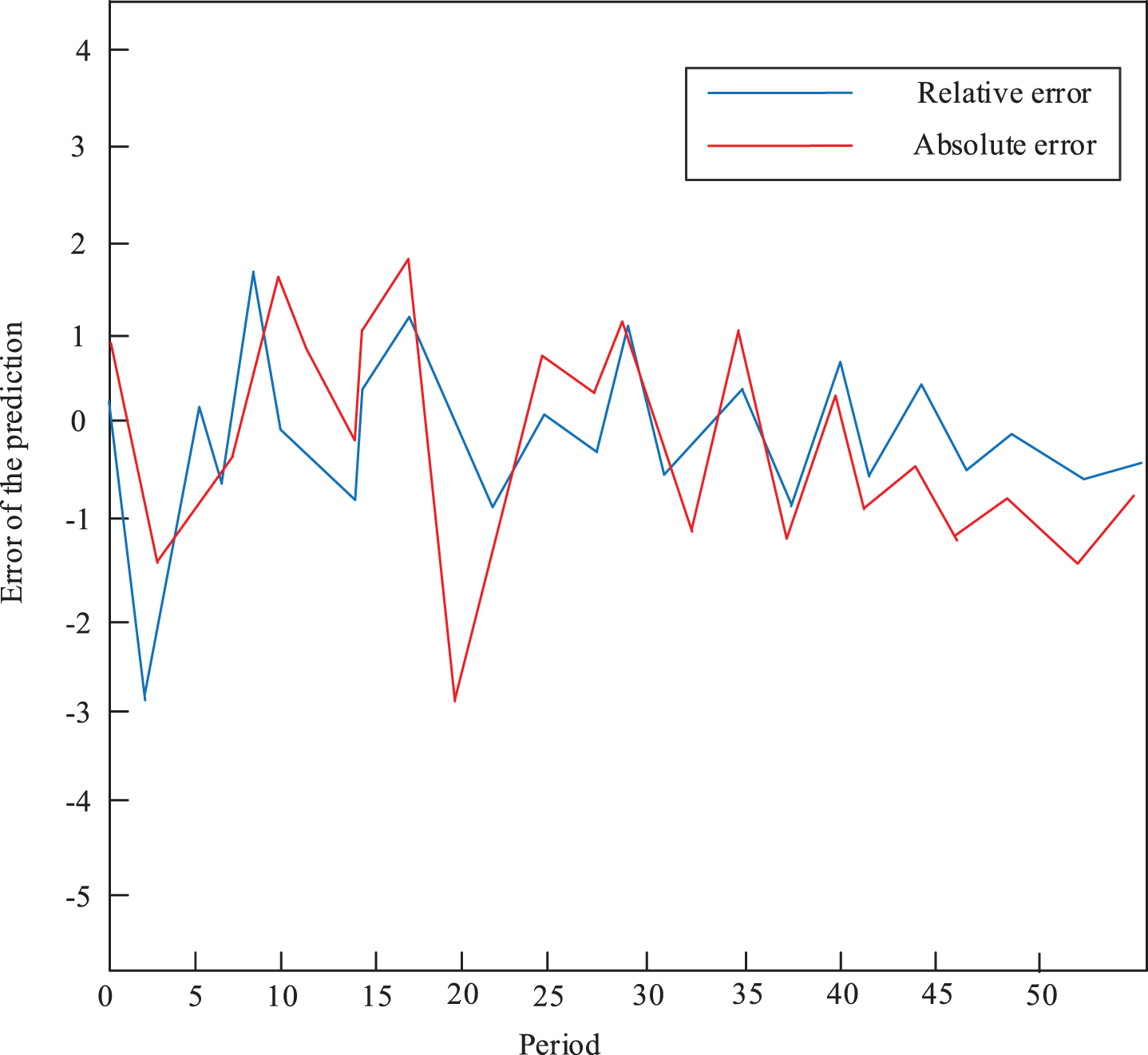
The error of the prediction of the BP algorithm.

4.2 Fitting effect and accuracy analysis of BP neural network model optimized based on IWPSO algorithm

Aiming at the shortcomings of a single BP network model, the method is proposed. Firstly, a randomness is selected for the initial inertia weight, and then an adaptive mutation operation is introduced to interfere with the particles that have been trapped in the local optimum to make it jump out of the local optimum and continue to optimize. This improves the optimization performance of the particle swarm algorithm. Finally, BP is trained. The basic control elements of the IWPSO optimized BP used are shown in Table 2.

Table 2
Basic control elements of the algorithm

Algorithm Basic elements Control value

IWPSO Population size 40

The maximum number of iterations 200

Particle length 30

Adaptive range of inertia weights 0.5∼0.9

Learning factor C1 = c2 = 2

BP Training goal 0.0001

Learning rate 0.01

Maximum learning times 500

Hidden layer tansing

Output layer puerline

Algorithm	Basic elements	Control value
IWPSO	Population size	40
	The maximum number of iterations	200
	Particle length	30
	Adaptive range of inertia weights	0.5∼0.9
	Learning factor	C1 = c2 = 2
BP	Training goal	0.0001
	Learning rate	0.01
	Maximum learning times	500
	Hidden layer	tansing
	Output layer	puerline

In order to analyze the fitting and prediction effects of the established IWPSO-optimized BP neural network model, this paper analyzes the fitting effect and fitting accuracy. Figure 9 is a comparison of measured and predicted training samples of BP neural network optimized by IWPSO. It can be intuitively seen that the measured curve of the displacement value and the predicted curve almost coincide, which also shows the fitting effect of the IWPSO optimized BP network model proposed in this paper better.

Comparing Fig. 9 with Fig. 7, we can see that the BP algorithm based on IWPSO optimization has a better fitting effect than the un-optimized BP algorithm. We can know the improved PSO has optimized training effect of the BP.

Fig.9

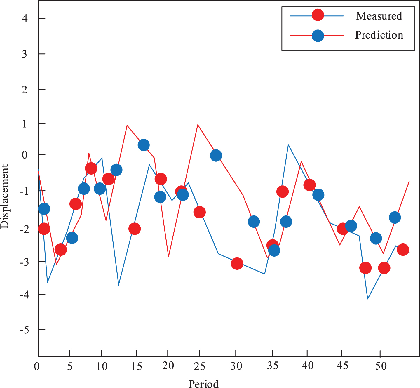
IWPSO-optimized BP neural network model prediction algorithm fitting effect diagram.

Figure 10 represents absolute error graph and the relative error graph of the BP network fitting based on IWPSO optimization. From Fig. 10 that the absolute error of BP based on IWPSO optimization is controlled within 0.5 mm. This shows that the fitting accuracy of the BP network model based on IWPSO optimization is higher.

Fig.10

IWPSO-optimized BP neural network model fitted absolute error plot.

4.3 Prediction accuracy analysis of BP model with multiple optimization algorithms

The BP neural network of the IWPSO and BP network of mutant particle swarm optimization (MPSO) proposed by [30], the BP neural network of adaptive mutant particle swarm optimization (AMPSO) proposed by [31], and literature [32] The proposed BP network learning algorithm of adaptive particle swarm optimization (MBPPSO) is compared.

MPSO algorithm parameters: population size is 10 and evolutionary algebra is 10.

AMPSO algorithm parameters: the number of particles is 30, the number of iterations is 40, the position upper and lower limits is [–1, 1], the speed upper and lower limits is [-200, 200], the cross probability is 0.9, and the size of the hybridization pool is 0.2.

MBPPSO algorithm parameters: the number of particles is 30; the number of iterations is 40. The maximum number of neural network trainings is set to 600.

In order to express, directly the prediction accuracy, see Fig. 11, error graphs of predictions of four different optimization algorithms are shown. It can be seen from the Fig. 11 that the absolute errors of all the predicted values are controlled within 0.65 mm; as shown in Fig. 12 do four different optimization algorithms predict the relative error maps of the network models, and the relative errors do not exceed 20%.

Fig.11

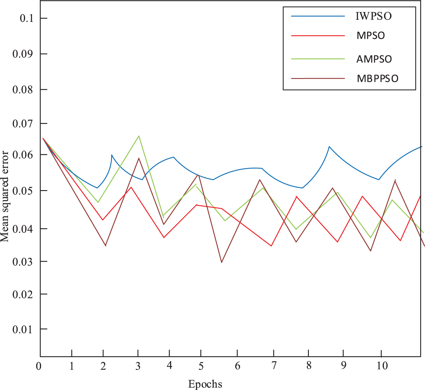
The prediction error graph of BP network model for different optimization algorithms.

Fig.12

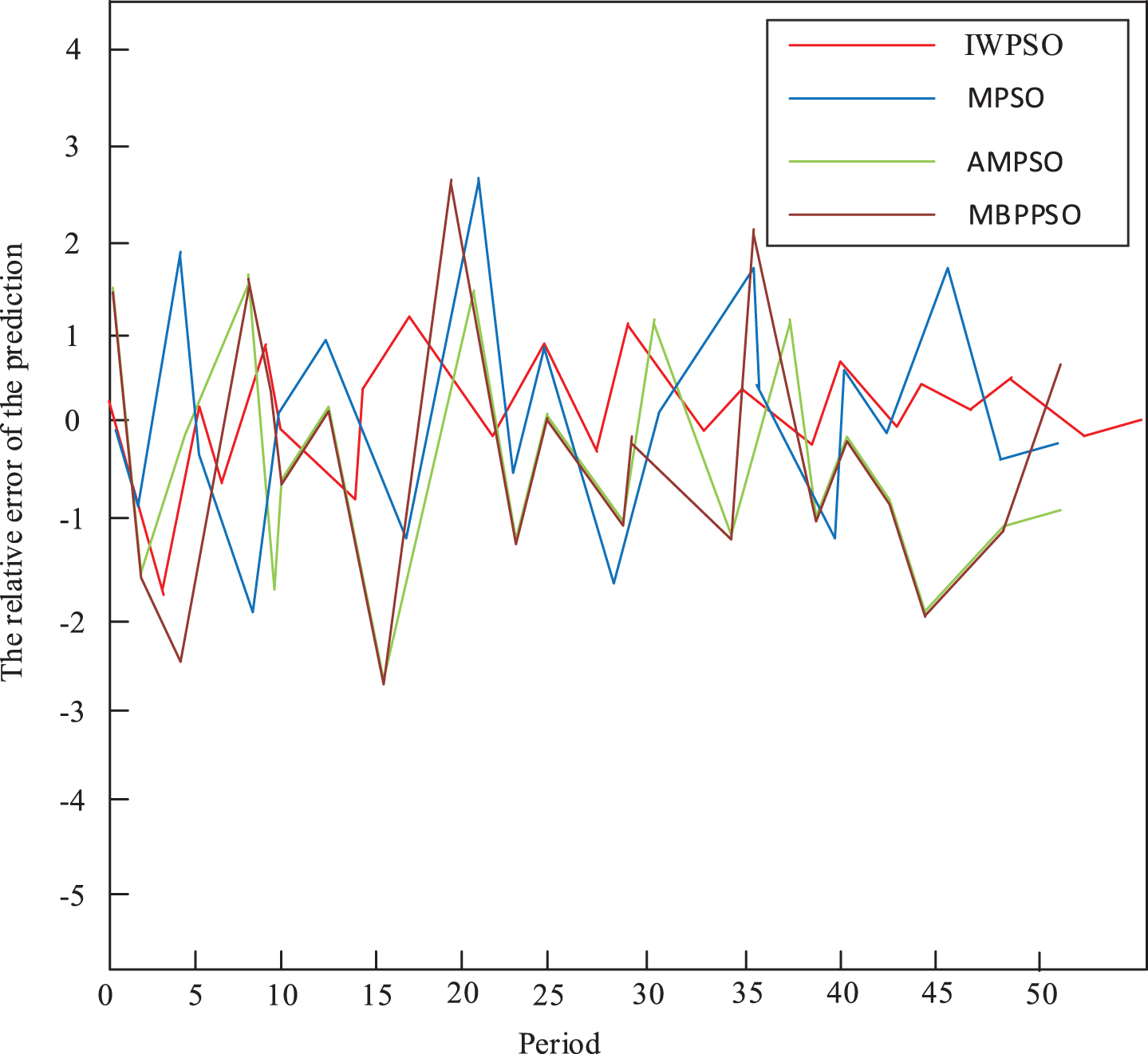
Relative error plots of BP network model fitting with different optimization algorithms.

From Fig. 12, IWPSO has higher prediction accuracy than BP network of the other optimization algorithms. Compared with Figs. 8 and 10, the prediction accuracy of IWPSO is higher than the accuracy of other three methods. The difference between the predicted value and the actual value is too large. Prediction effect of IWPSO is significantly better than single BP network, and it is better than that of the other optimization algorithms.

5 Conclusion

Aiming at the precocious convergence, low search accuracy and easy divergence of most particle swarm optimization algorithms with velocity terms, this paper proposes a random inertia weights and quantization (IWPSO). The learning factor adopts a strategy that changes asynchronously. Simulation results indicate that our method has significantly improved search speed, convergence accuracy and stability compared with existing improved algorithms, and has the ability to get rid of being trapped in a local optimal solution. At the same time, the method has good stability. Therefore, the IWPSO algorithm is an efficient particle swarm optimization because of its own characteristics of the algorithm model, which has better global convergence performance than the general PSO algorithm.

References

Carleo

and Troyer

, Solving the quantum many-body problem with artificial neural networks[J], Science 355(6325) (2017), 602–606.

Andreatta

and Nielsen

, Gapped sequence alignment using artificial neural networks: application to the MHC class I system[J], Bioinformatics 32(4) (2016), 511–517.

Tkáč

and Verner

, Artificial neural networks in business: Two decades of research[J], Applied Soft Computing 38 (2016), 788–804.

Chen

, Challita

, Saad

, et al., Artificial neural networks-based machine learning for wireless networks: A tutorial[J], IEEE Communications Surveys & Tutorials 21(4) (2019), 3039–3071.

Chine

, Mellit

, Lughi

, et al., A novel fault diagnosis technique for photovoltaic systems based on artificial neural networks[J], Renewable Energy 90 (2016), 501–512.

Wang

, Zhang

, Wu

, et al., Wind speed forecasting based on the hybrid ensemble empirical mode decomposition and GA-BP neural network method[J], Renewable Energy 94 (2016), 629–636.

Wang

, Luo

, Grunder

, et al., Multi-step ahead electricity price forecasting using a hybrid model based on two-layer decomposition technique and BP neural network optimized by firefly algorithm[J], Applied Energy 190 (2017), 390–407.

, Zhou

, Chen

, et al., Supercritical water heat transfer coefficient prediction analysis based on BP neural network[J], Nuclear Engineering and Design 320 (2017), 400–408.

Cao

, Wang

, Ming

, et al., A review on neural networks with random weights[J], Neurocomputing 275 (2018), 278–287.

10.

Wang

L.J.

, Ji

S.F.

and Ji

N.Y.

, Application of CSA-BP neural network in gearbox fault diagnosis[J], International Journal of Circuits, Systems and Signal Processing 13 (2019), 273–280.

11.

Jiang

, Huang

, et al., Application of BP Neural Network Based on Genetic Algorithm Optimization in Evaluation of Power Grid Investment Risk[J], IEEE Access 7 (2019), 154827–154835.

12.

Tharwat

, Elhoseny

, Hassanien

A.E.

, et al., Intelligent Bézier curve-based path planning model using Chaotic Particle Swarm Optimization algorithm[J], Cluster Computing 22(2) (2019), 4745–4766.

13.

Deng

, Xu

and Zhao

, An improved ant colony optimization algorithm based on hybrid strategies for scheduling problem[J], IEEE Access 7 (2019), 20281–20292.

14.

Chi

, Su

, Zhang

, et al., A hybridization of cuckoo search and particle swarm optimization for solving optimization problems[J], Neural Computing and Applications 31(1) (2019), 653–670.

15.

Hao

, Wang

, Shan

, et al., Prediction of electricity consumption in cement production: a time-varying delay deep belief network prediction method[J], Neural Computing and Applications 31(11) (2019), 7165–7179.

16.

Liang

, Xu

, Bao

, et al., Barzilai–Borwein-based adaptive learning rate for deep learning[J], Pattern Recognition Letters 128 (2019), 197–203.

17.

Liu

, Hu

and Hong

, Electric Energy Substitution Potential Prediction Based on Logistic Curve Fitting and Improved BP Neural Network Algorithm[J], Elektronika ir Elektrotechnika 25(3) (2019), 18–24.

18.

Heravi

A.R.

and Hodtani

G.A.

, A new and fast correntropy-based method for system identification with exemplifications in low-SNR communications regime[J], Neural Computing and Applications 31(8) (2019), 4407–4422.

19.

Tang

X.L.

, Ma

W.C.

, Kong

D.S.

, et al., Semisupervised deep stacking network with adaptive learning rate strategy for motor imagery eeg recognition[J], Neural Computation 31(5) (2019), 919–942.

20.

Saffaran

, Moghaddam

M.A.

and Kolahan

, Optimization of backpropagation neural network-based models in EDM process using particle swarm optimization and simulated annealing algorithms[J], Journal of the Brazilian Society of Mechanical Sciences and Engineering 42(1) (2020), 1–14.

21.

Yao

, Yin

, Shi

, et al., Stress detection based on electromagnetic fusion and deep belief network optimised by a simulated annealing algorithm[J], Insight-Non-Destructive Testing and Condition Monitoring 61(7) (2019), 404–411.

22.

Y.X.

, Niu

L.C.

, Yang

, et al., Optimization of Lithium Battery Pole Piece Thickness Control System Based on GA-BP Neural Network[J], Journal of Nanoelectronics and Optoelectronics 14(7) (2019), 978–986.

23.

Liu

, Wei

, Zhang

, et al., Analysis of epileptic seizure detection method based on improved genetic algorithm optimization back propagation neural network[J], Journal of Biomedical Engineering=Shengwu Yixue Gongchengxue Zazhi 36(1) (2019), 24–32.

24.

Nagra

A.A.

, Han

and Ling

Q.H.

, An improved hybrid self-inertia weight adaptive particle swarm optimization algorithm with local search[J], Engineering Optimization 51(7) (2019), 1115–1132.

25.

, Chen

, Wang

, et al., An improved particle swarm optimization algorithm with adaptive inertia weights[J], International Journal of Information Technology & Decision Making 18(03) (2019), 833–866.

26.

Zeng

H.Y.

, Improved Particle Swarm Optimization Based on Tabu Search for VRP[J], Journal of Applied Science and Engineering Innovation 6(2) (2019), 99–103.

27.

Harrison

K.R.

, Ombuki-Berman

B.M.

and Engelbrecht

A.P.

, A parameter-free particle swarm optimization algorithm using performance classifiers[J], Information Sciences 503 (2019), 381–400.

28.

Wang

, Research on Particle Swarm Optimization Algorithm Based on Quantum Computing Technology[J], American Journal of Electrical and Electronic Engineering 8(1) (2020), 21–25.

29.

Chen

, Zhou

F.Y.

and Yuan

X.F.

, Hybrid particle swarm optimization with spiral-shaped mechanism for feature selection[J], Expert Systems with Applications 128 (2019), 140–156.

30.

Lalwani

, Sharma

, Satapathy

S.C.

, et al., A survey on parallel particle swarm optimization algorithms[J], Arabian Journal for Science and Engineering 44(4) (2019), 2899–2923.

31.

, Zhang

, et al., Temperature Compensation of Piezo-Resistive Pressure Sensor Utilizing Ensemble AMPSO-SVR Based on Improved Adaboost. RT[J], IEEE Access 8 (2020), 12413–12425.

32.

Qiao

J.F.

, Lu

and Li

W.J.

, Design of dynamic modular neural network based on adaptive particle swarm optimization algorithm[J], IEEE Access 6 (2018), 10850–10857.

33.

Jia

, Zhao

, Zheng

, et al., A novel optimized GA–Elman neural network algorithm[J], Neural Computing and Applications 31(2) (2019), 449–459.

34.

, Gao

and Yang

, Prediction of coal and gas outburst: A method based on the BP neural network optimized by GASA[J], Process Safety and Environmental Protection 133 (2020), 64–72.

35.

Zhang

, Xie

S.F.

, Zhou

Z.H.

, et al., Prediction of PM 2.5 Concentration of BP Neural Network Based on Improved Particle Group Algorithm[J], The International Archives of Photogrammetry, Remote Sensing and Spatial Information Sciences 42 (2020), 173–178.

36.

, Yin

and Liu

, A Novel Heuristic Artificial Neural Network Model for Urban Computing[J], IEEE Access 7 (2019), 183751–183760.

37.

Zhang

, Application of improved BP neural network based on e-commerce supply chain network data in the forecast of aquatic product export volume[J], Cognitive Systems Research 57 (2019), 228–235.

38.

Liu

, Zhou

, Wang

, et al., A BP neural network-based communication blind signal detection method with cyber-physical-social systems[J], IEEE Access 6 (2018), 43920–43935.

39.

Zhu

, Wei

and Xiao

, Fault diagnosis of neural network classified signal fractal feature based on SVM[J], Cluster Computing 22(2) (2019), 4249–4254.

40.

Wen

, Xiao

, Yang

, et al., Adjusting learning rate of memristor-based multilayer neural networks via fuzzy method[J], IEEE Transactions on Computer-Aided Design of Integrated Circuits and Systems 38(6) (2018), 1084–1094.

41.

Zhao

, Xu

and Jia

, Improved shuffled frog leaping algorithm-based BP neural network and its application in bearing early fault diagnosis[J], Neural Computing and Applications 27(2) (2016), 375–385.

42.

Liu

and Yin

, An improved particle swarm optimization algorithm used for BP neural network and multimedia course-ware evaluation[J], Multimedia Tools and Applications 76(9) (2017), 11961–11974.

43.

Piotrowski

A.P.

, Napiorkowski

M.J.

, Napiorkowski

J.J.

, et al., Swarm intelligence and evolutionary algorithms: Performance versus speed[J], Information Sciences 384 (2017), 34–85.

Optimization of artificial CNN based on swarm intelligence algorithm

Abstract

Keywords

1 Introduction

2 BP network

2.1 Principle of BP network

3 BP neural network optimization based on PSO

3.1 Basic PSO

4.1 Fitting effect and accuracy analysis of un-optimized BP network

Table 1 BP neural network training parameters Training times Training goal Learning rate 500 0.0001 0.01

References

Table 1
BP neural network training parameters

Training times Training goal Learning rate

500 0.0001 0.01