Spatial possibilistic fuzzy C-Mean segmentation method integrated with brain Mid-Sagittal Surface information extracted by an evolutionary algorithm

Abstract

A normal human brain holds a high level of bilateral reflection symmetry. On the sagittal view, the brain can be separated into the left and the right hemispheres with approximately identical anatomical properties, so that symmetrical mirror pixels are almost similar. As a result, the symmetry information can be used to enhance results of brain segmentation methods. In this paper, I introduced a new version of the Fuzzy C-Mean (FCM) segmentation method which is called Genetic Spatial Possibilistic Fuzzy C-Mean (GSPFCM). GSPFCM integrates symmetry information with SPFCM. It is an extension of Possibilistic Fuzzy C-Mean (PFCM) on 3D Magnetic Resonance (MR) images. GSPFCM uses the spatial information and fuzzy membership values. Spatial and possibilistic information were added in order to solve the noise sensibility defect of FCM. To integrate the symmetry information, I first extracted the Mid-Sagittal Surface using a proposed genetic algorithm. According to this algorithm, inside each axial slice, a Thin-Plate Spline (TPS) surface was constructed and a genetic algorithm was applied to fit this TPS surface to the brain data. Then, the symmetry degree of each symmetry pair voxels was calculated. Finally, the membership values in SPFCM were updated based on the corresponding symmetrical values. The efficiency of GSPFCM, was evaluated using both simulated and real Magnetic Resonance Images (MRI), and was compared to the state-of-the-art methods. My results showed images with different degrees of Intensity Non-Uniformity (INU) and different levels of noise were segmented efficiently by the GSPFCM.

Keywords

3D brain MR segmentation Mid-Sagittal Surface Fuzzy C-Mean genetic algorithm fractal dimension possibilistic information spatial information

1 Introduction

Image segmentation is an important step in image analysis. From all types of image-segmentation methods, Fuzzy C-Mean (FCM) clustering algorithm is a rather old method, which has been commonly used in image segmentation [3]. FCM is a cluster-based segmentation method. It assigns voxels in an image to different classes according to the distance of their features with the classes [3, 4]. Nevertheless, this method suffers from a number of problems; Noise sensitiveness [5], use of Euclidian distance as the similarity criterion of data points which leads to a limitation of equal partition trend for datasets [6], and high-time complexity are the main problems of conventional FCM [7_ENREF_7]. A large number of researches have been conducted to overcome these problems. These endeavors mostly include updating the objective function of FCM, or adding some terms to this function. The involved information for this purpose includes spatial information [5], grey information [7], cluster density [6], belief concept [8], and symmetry information [4].

When a data element is very far from the fuzzy centroids, for example a noise, FCM classifies this data to the nearest class, based on the distance between this data value and the centroids of the classes. Also, the centroids are updated so that they get nearer to this noisy data. It means the next data are classified based on the centroids being influenced by a noisy value, which leads to a less accurate classification result. A possibi1istic concept is used to face this problem; in a classifier using possibi1istic values, membership value of a data in a cluster (or class) represents the typicality of the voxel in the class, or the possibility of the voxel belonging to the class [9]. Possibi1istic C-Mean (PCM) assigns data values into different classes according to their possibi1istic values. PCM solves the noise sensibility defect of FCM, but it suffers from the coincident cluster problem [10]. A classifier which works using a combination of fuzzy membership values and possibilistic values seems to be a more practical classifier. In [10], Pal et al. proposed Fuzzy PCM. FPCM is a combination of relative (or membership) and absolute typicalities (or possibilities). Pal et al. improved their method by adding a new penalty to the objective function in order to suppress the noise affects. The new method was called PFCM [11].

On the other hand, a normal human brain holds a high level of bilateral reflection symmetry; a highly convolved brain can be separated into the left and the right hemispheres by the Inter-hemispheric Fissure (IF), or the longitudinal fissure, which is a long and deep furrow (see Fig. 1). Corresponding regions of two hemispheres have approximately identical anatomical properties, and also have comparable, if not identical, physiologic (e.g., blood perfusion) properties [12]. Owing to this high identicalness, the plane that passes vertically through this midline is considered to be the Mid-Sagittal Plane (MSP).

Fig. 1

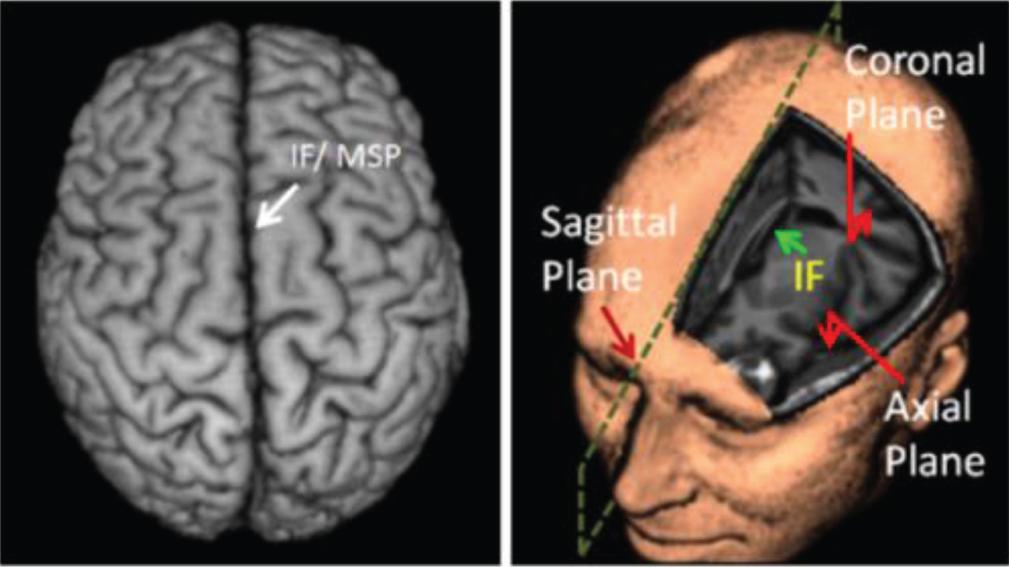
Human brain exhibits approximate bilateral symmetry (Image from [1]).

Incorporation of symmetry into generalized image segmentation is still immature [4, 13]. To the best of my knowledge, this kind of use of symmetry information can be traced back to the 1993 work of [14]. In this work, symmetry was used to reduce the redundancy in the images. In [15], using the symmetry information, the segmentation problem was formulated as a minimizer goodness of the fitness function. In [16], colour and symmetry were utilized to detect regions of interest (ROI) in an image. In [17], in order to find symmetric regions, global symmetry was integrated into the edge weights of the normalized cut (n-cut) segmentation. In [18], local symmetry was combined with an objective function of the level-set segmentation, to segment the boundary of the symmetric objects. And finally, in [13], bilateral symmetry was integrated into the image-segmentation algorithm, based on region-growing technique.

Symmetry information has been also used in brain MR image segmentation. In [12, 19], brain image segmentation was carried out to detect the existence and the outlines of tumours, based on the symmetry character of brain MRI image and its edge information. In [20], a symmetry-integrated brain injury detection method was presented. In this method, a symmetry affinity matrix was used to segment the brain slices, potential asymmetric regions were detected, a 3D relaxation algorithm was applied to the cluster pixels in the symmetry affinity matrix, and asymmetric regions were refined. Brain injuries were finally extracted. In [21], symmetry plane was used to determine asymmetric areas in the brain which was helpful to detect tumours. And finally, in [22], a fuzzy point symmetry-based genetic clustering was introduced to segment the brain image. In that work, the search capability of the genetic algorithm was utilized for automatically evolving the clusters’ centroids. Assignment of points to different clusters was made based on the point symmetry-based distance. A fuzzy point symmetry-based cluster validity index was used as a measure of ‘goodness’ of the corresponding partitions.

As a more accurate alternative concept for MSP, the Mid-Sagittal Surface (MSS) is a (curved) surface corresponding with the IF and separating the two hemispheres. Contrary to the MSP, the MSS has potential to be consistent with the natural shape of the IF. In the presence of asymmetries, caused either by natural variation or pathology, a MSS is able to correctly separate two hemispheres, whereas an MSP would intersect or misclassify some brain tissues [23]. This is illustrated in Fig. 2 where the Mid-Sagittal Plane (dotted line) and the manually delineated Mid-Sagittal Surface (solid line) are not matched.

Fig. 2

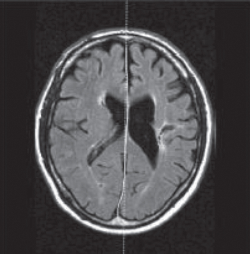
Example scan showing difference between the MSP (dotted line) and the manually delineated MSS (solid line) (Image from [2]).

In this research, I had two contributions; first I introduced SPFCM as a new version of PFCM which combines spatial values and possibilistic concept with fuzzy membership values. SPFCM was introduced in an attempt to handle the noise and Intensity Non-Uniformity (INU) effect. Second, I applied symmetry information to SPFCM. For this purpose, I introduced a genetic algorithm to extract the Mid-Sagittal Surface. Using the extracted MSS, I determined the symmetry pairs, and the symmetry degree of each pair. In the next steps, I injected the calculated symmetry degrees to the SPFCM objective function, and I amended the updating formulas of the centroids, as well as membership values in each class based on this new objective function. As a result, I have a classifier method called GSPFCM, which uses membership information, possibilistic information, spatial information, and symmetry information.

2 The genetic symmetry-integrated SPFCM

General view of the proposed segmentation method, GSPFCM is as follows (see Fig. 3). First of all, Spatial Possibilistic Fuzzy C-Mean (SPFCM) is modelled. SPFCM is used as the clustering model. In the next step, in order to apply symmetry information to the SPFCM, Mid-Sagittal Surface is estimated, Symmetry-Pairs are obtained, and symmetry information is applied to SPFCM. For the last purpose, Symmetry Degrees are calculated, and GSPFCM objective function, centroids’ updating formula, membership values’ updating formula, and possibilistic values’ updating formula are calculated. Each step is more described in the next sections.

Fig. 3

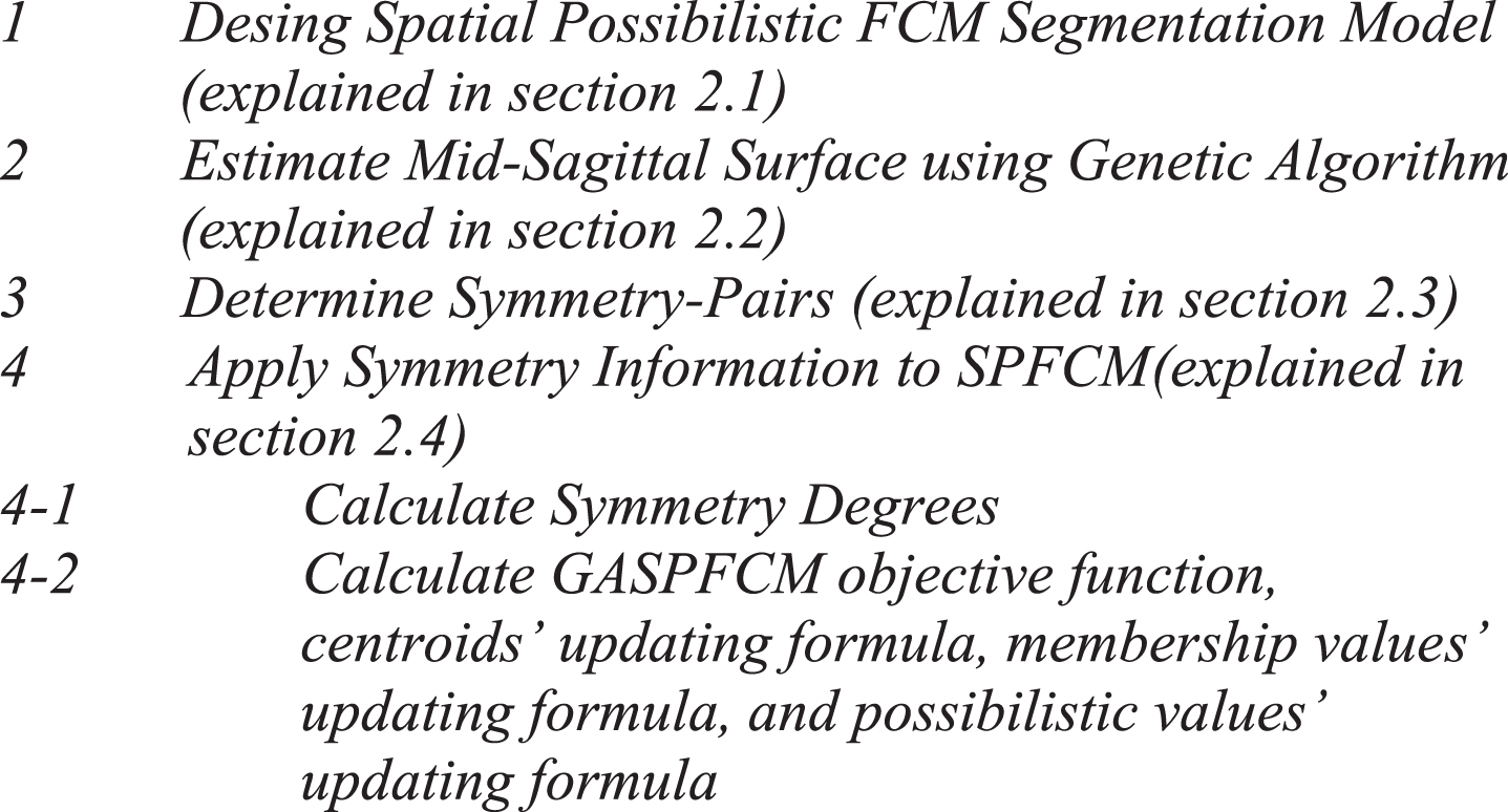
Pseudo code of the proposed GASPFCM segmentation method.

2.1 The spatial possibilistic FCM

SPFCM is an extension of FCM [24] and PFCM [11]. SPFCM takes into account of both possibilistic and membership values in the form of an optimization solution. In SPFCM, the local spatial continuity is applied to calculate the proximities [25].

The objective function for the SPFCM clustering algorithm is given by $\begin{matrix} J_{SPFCM} = \sum_{\underline{x} \in I} \sum_{k = 1}^{c} ({au}_{k, \underline{x}}^{m} + a^{,} t_{k, \underline{x}}^{n}) D_{k, \underline{x}} + \sum_{k = 1}^{c} η_{k} \\ \sum_{\underline{x} \in I} {(1 - t_{k, \underline{x}})}^{n} + β η (w_{z} (x, y)) + γ φ (w_{z} (x, y)) \end{matrix}$ (1) where m ∈ (1, ∞) is the fuzzy index,n ∈ (1, ∞) is the possibilistic index, c is the total number of clusters, and $u_{k, \underline{x}}$ refers to the membership degrees of pixel $s (\underline{x})$ in the kth cluster. The constraints $a > 0, a^{,} > 0, 0 ⩽ u_{k, \underline{x}}^{m}, t_{k, \underline{x}}^{n} ⩽ 1, η_{k} > 0, \sum_{\underline{x} \in I} t_{k, \underline{x}} = 1 \forall k$ , and $\sum_{k = 1}^{c} u_{k, \underline{x}} = 1 \forall \underline{x} \in I$ . The parameters a and a′, make a balance between effect of possibilistic concept and membership values. $t_{k, \underline{x}}$ refers to the probabilistic value $s (\underline{x})$ at the kth cluster c_k. Finally, let $w (\underline{x}) = log \tilde{b} (\underline{x})$ where $\tilde{b} (\underline{x})$ is an estimate for the unknown bias field $b (\underline{x})$ . The 3D log bias field $w (\underline{x})$ is modeled as a stack of 2D spline surfaces {w_z (x, y)}, where each of the spline surfaces w_z (x, y) is computed over the 2D x - y plane at the particular z index. The parameters β and γ control the fidelity of the fit to the bias data and the smoothness of the bias field. η (w_z (x, y)) minimizes the thin plate energy of each spline surface w_z (x, y) and φ (w_z (x, y)) smooths slices between spline surfaces. They are calculated as follows [26]. $\begin{matrix} η (w_{z} (x, y)) = \\ \iint {{[\frac{\partial^{2} w_{z} (x, y)}{\partial x^{2}}]}^{2} + 2 {[\frac{\partial^{2} w_{z} (x, y)}{\partial x \partial y}]}^{2} + {[\frac{\partial^{2} w_{z} (x, y)}{\partial y^{2}}]}^{2}} dxdy \end{matrix}$ (2) $φ (w_{z} (x, y)) = \iint {[\frac{\partial^{2} w_{z} (x, y)}{\partial z^{2}}]}^{2} dxdy$ (3) $d_{k, \underline{x}}^{2}$ gives the Euclidian distance between $s (\underline{x})$ as the measured MR image signal ( $s (\underline{x}) = o (\underline{x}) b (\underline{x}) + n (\underline{x})$ where $o (\underline{x})$ is the true signal emitted by the tissue, $b (\underline{x})$ is the unknown smoothly varying bias field, and $n (\underline{x})$ is an additive noise assumed to be independent of $b (\underline{x})$ ) and the centre of the kth cluster c_k. $D_{k, \underline{x}} = \frac{1}{| ℵ_{\underline{x}} |} \sum_{\underline{y} \in ℵ_{\underline{x}}} [d_{k, \underline{x}}^{2} λ_{\underline{x}, \underline{y}} + d_{k, \underline{y}}^{2} (1 - λ_{\underline{x}, \underline{y}})]$ (4) $d_{k, \underline{x}}^{2} = \frac{s (\underline{x})}{\tilde{b} (\underline{x})} - v_{k}^{2}$ (5)

ℵ is a neighbourhood of the $s (\underline{x})$ , $| ℵ_{\underline{x}} |$ is the cardinality of ℵ, and $λ (\partial_{\underline{x}, \underline{y}}) = λ_{\underline{x}, \underline{y}}$ is the weighting factor controlling the influence degree of the neighbouring voxels $s (\underline{y}) \in ℵ_{\underline{x}}$ on the centre voxel $s (\underline{x})$ , defined by $λ (\partial) = \frac{1}{1 + e^{- (\partial - μ) / δ}}$ (6)μ and δ are the average and the standard deviation of $s (\underline{y}) \in ℵ_{\underline{x}}$ , respectively, and ∂ refers to the difference between $s (\underline{x})$ and its neighbor $s (\underline{y})$ .

The necessary conditions for the minimization of J_SPFCM over the membership $u_{k, \underline{x}}$ , possibilistic values $t_{k, \underline{x}}$ , and cluster centroids v_k are obtained by setting the respective first partial derivatives of J_SPFCM to zero while keeping the other variables constant. Considering Lagrange functional yields: $t_{k, \underline{x}} = \frac{1}{1 + {(a^{,} \times \frac{D_{k, \underline{x}}^{2}}{η_{k}})}^{\frac{1}{n - 1}}}$ (7) $u_{k, \underline{x}} = {[\sum_{l = 1}^{c} {(\frac{D_{k, \underline{x}}}{D_{l, \underline{x}}})}^{1 / m - 1}]}^{- 1}$ (8) $v_{k} = \frac{\sum_{\underline{x} \in I} (a u_{k, \underline{x}}^{m} + a^{,} t_{k, \underline{x}}^{n}) g_{\underline{x}}}{\sum_{\underline{x} \in I} (a u_{k, \underline{x}}^{m} + a^{,} t_{k, \underline{x}}^{n})}$ (9) where

$g_{\underline{x}} = \frac{1}{| ℵ_{\underline{x}} |} \sum_{\underline{y} \in ℵ_{\underline{x}}} [λ_{\underline{x}, \underline{y}} (\frac{s (\underline{x})}{\tilde{b} (\underline{x})}) + (1 - λ_{\underline{x}, \underline{y}}) (\frac{s (\underline{y})}{\tilde{b} (\underline{y})})]$ (10) $η_{k} = K \frac{Σ_{\underline{X} \in I} u_{k, \underline{x}}^{n} D_{k, \underline{x}}^{2}}{Σ_{\underline{x} \in I} u_{k, \underline{x}}^{n}}$ (11)η_k are constraints; the typicality values are strongly dependent on the values of η_k; if η_k is low, $t_{k, \underline{x}}$ will be small, and if η_k is high, $t_{k, \underline{x}}$ will be high.

2.2 Mid-sagittal surface extraction method

A high-level pseudo code of my MSS extraction method is presented in Fig. 4. In this algorithm, an initial MSP is estimated (line 1 of the pseudo code). Genetic algorithm is applied and the best chromosome expressing the most proper control points is achieved (lines 2 to 10). Finally, MSS is constructed crossing the selected control points using TPS (line 11).

Fig. 4

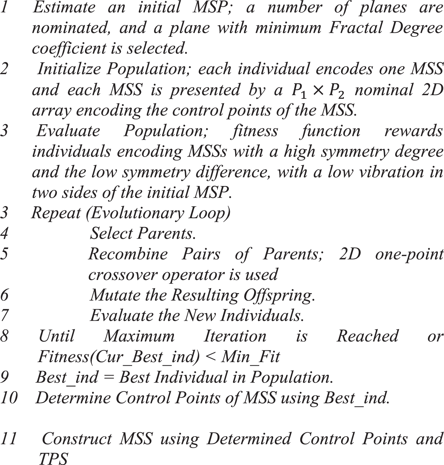
Pseudo code of the proposed MSS extraction method.

First, an initial Mid-Sagittal Plane is estimated. For this purpose, a number of planes in the middle of the brain in sagittal view with limited number of coronal and axial rotation degrees are nominated, and among these nominated planes, a plane with minimum Fractal Degree (FD) coefficient, α, (as the same definition as Equation 2) value is selected. FD value is calculated for each box with variable size moving through both cerebral hemispheres. After detecting initial MSP according to a texture information, FD, which is fast and noise free, I calculate Correlation Coefficient (CC) for a very limited number of plate (two plates in each side) around the extracted MSP. The initial MSP is a plane with the minimum CC value. CC is calculated for all symmetry pairs in the cerebral hemispheres and using the pixels’ intensity values. This makes CC ineffective in Pathological images. In addition, determining pairs and calculating CC is time consuming compared to FD [27].

In the next step, candidate positions are selected. For this purpose, a genetic algorithm with the specifics explained before is applied. The output of this section is a chromosome consisting of a 2D array with P₁ × P₂ elements. Providing the volume of the chromosome which is much less than size of main image, time complexity is not more a constrain for my algorithm. The control points for constructing the Thin-Plate Surface are achieved from the resulted chromosome.

For the selected control points, a Thin-Plate Surface is constructed. The corresponding pixel values of the final Mid-Sagittal Surface including the selected ones, as the control points, and the others are calculated using the extracted TPS. In order to construct the Thin-Plate Spline instead of applying matrix inversion process which brings an extensive time complexity, Singular Value Decomposition (SVD) is used [26].

2.2.1 Genetic algorithm (GA) encoding of MSS

In my genetic algorithm, each individual of the population encodes one MSS and each MSS is presented by a P₁ × P₂ nominal 2D array encoding the control points of the MSS. P₁ and P₂ are the number of points in axial and coronal axes of the MSS (see Fig. 5). These control points in each line will be used to construct corresponding Thin-Plane Splines. According to [28], the number of points participating in this construction should be between 5 to 9. Thus, P₁ and P₂ are assigned to a value in this limitation. I set P₁ and P₁ with 7 and 6 respectively. These low values decrees size of chromosomes and enhance dramatically the speed of the genetic algorithm. Figure 5 shows genotype structure of a chromosome. While sub-figure (a) presents a chromosome, sub-figure (b) shows how the genes’ values are interpreted. The initial population are assigned with random values.

Fig. 5

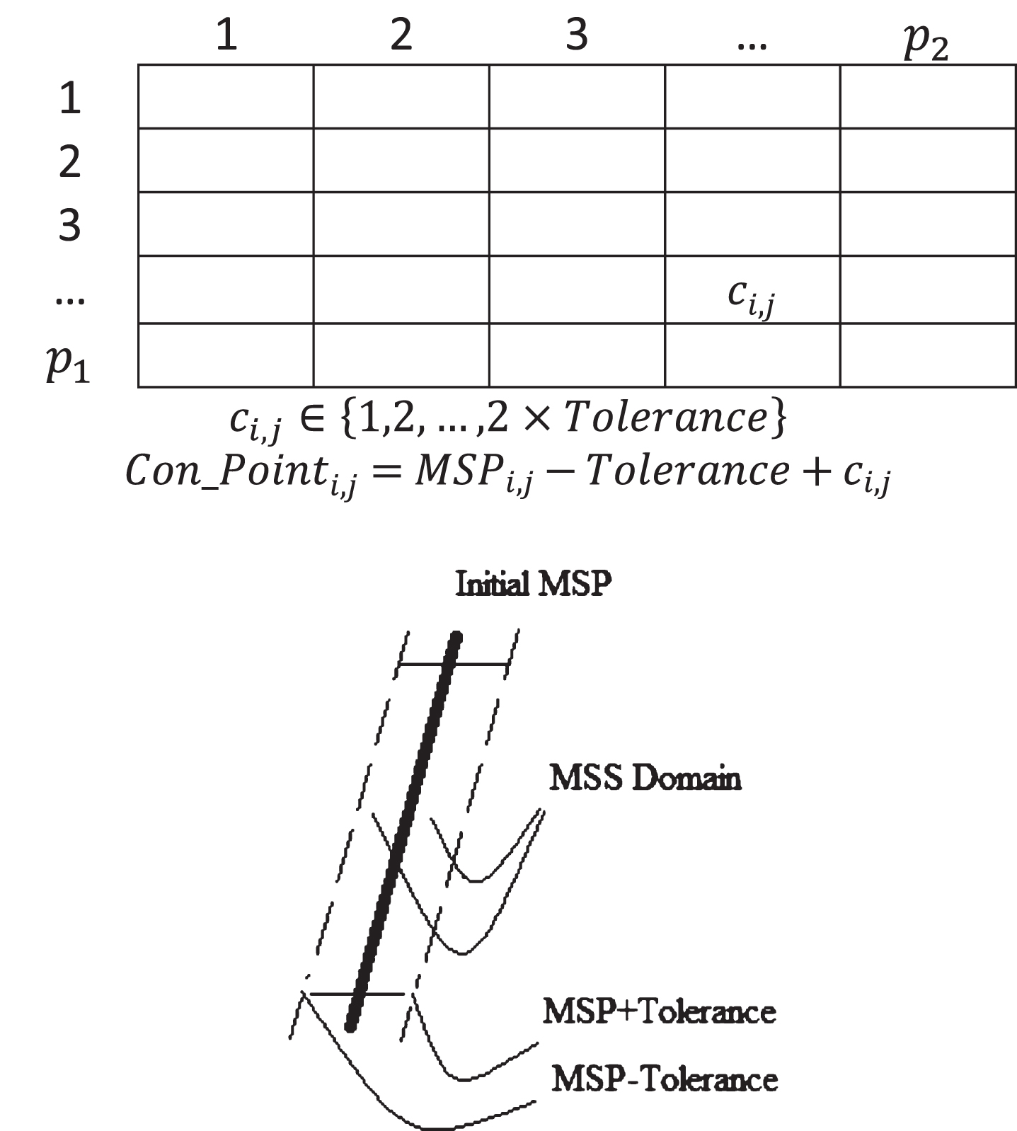
Structure of a Chromosome and its interpretation.

2.2.2 GA fitness function

The fitness function rewards individuals encoding MSSs with high symmetry degree and low symmetry difference, α, with low vibration in two sides of the initial MSP. To this aim the following fitness function is used: $f (X) = w_{1} α + w_{2} γ$ (12) where α presents the symmetry difference, and γ refers to the vibration in two sides of the initial MSP. w₁, and w₂ are two coefficients used to balance the double factors. α is calculated as following formula. $α = \frac{| {FD}_{L} - {FD}_{R} |}{| {FD}_{L} + {FD}_{R} |}$ (13) where FD_L and FD_R refer to the fractal dimension values for the left and right axial hemispheres, respectively.

My experiments showed that fitness function without considering the spatial information of the control points in each chromosome leads me to a jagged MSS. To address this problem, I added γ to the fitness function. γ is calculated based on Local Binary Pattern (LBP) concept and using the following equation. γ shows how much neighbour control points in the corresponding MSS are located in two sides of the initial MSP. $\begin{matrix} γ = \frac{1}{2 \times P_{1} \times P_{2}} \sum_{i = 1}^{P_{1}} \sum_{j = 1}^{P_{2}} s (c_{i, j}, c_{i, j + 1}) \\ + s (c_{i, j}, c_{i + 1, j}) \end{matrix}$ (14) where P₁ and P₂ refer to the size of chromosome, and c_i,j presents the element value per (i, j). Function s is calculated as follows. $s (a, b) = {\begin{matrix} 1 if | a - b | > Tolerance \\ 0 otherwise \end{matrix}$ (15)

2.2.3 Genetic operators

The individuals are selected for reproduction with a tournament selection operator; a number of individuals are randomly selected, and the one with lower fitness is chosen as elite. The number of selected individuals determines the size of the tournament. Elitism is applied with a given size. 2D one-point crossover operator is used; in short, one-point crossover selects a point inside the two chromosomes and produces the offspring by exchanging the substrings of the parents. Standard mutation operator is employed; a row number and a column number are selected randomly and value of the corresponding gene is changed with a random valid number.

2.2.4 GA parameters setting

As most Evolutionary Algorithms, my proposed genetic algorithm for MSS extraction uses several parameters that control the genetic search, e.g., crossover and mutation probabilities, population size, etc. In general, for an EA to perform well, the issue of setting the parameter values that are used to guide the genetic search is critical. I used the values as whatever shown in Table 1. These values have been achieved experimentally.

Table 1
GA Parameter values

Parameter Value Parameter Value

Population Size 30 Number of Generations 30

Crossover Probability 90 Mutation Probability 10

Elitism Size 10 Tournament Size 3

Tolerance 2 Min_Fit 0.015

w₂ (Weight of Vibration) 9 p₁ (Chromosome Length) 5

p₂ (Chromosome Height) 7 w₂ (Weight of Symmetry Diff.) 1

Parameter	Value	Parameter	Value
Population Size	30	Number of Generations	30
Crossover Probability	90	Mutation Probability	10
Elitism Size	10	Tournament Size	3
Tolerance	2	Min_Fit	0.015
w₂ (Weight of Vibration)	9	p₁ (Chromosome Length)	5
p₂ (Chromosome Height)	7	w₂ (Weight of Symmetry Diff.)	1

One of the potential problems of using evolutionary algorithms is the high time consumption problem. The time complexity of these algorithms mainly depends on the values of a number of control parameters including Population Size, Number of Generations, Size of Chromosomes (P₁ and P₂). The best values for these parameters make an optimal balance between performance and time complexity. They are dependent on the problems naturally and the way of designation of optimisation method. I set these parameters with the optimal values as they were achieved from Fig. 6. In each part of this figure I present a chart that shows the ratio of mean accuracy on time consumption via different values of the corresponding parameter in the horizontal axis. In these tests, when a parameter is investigated, all other parameters are constant.

Fig. 6

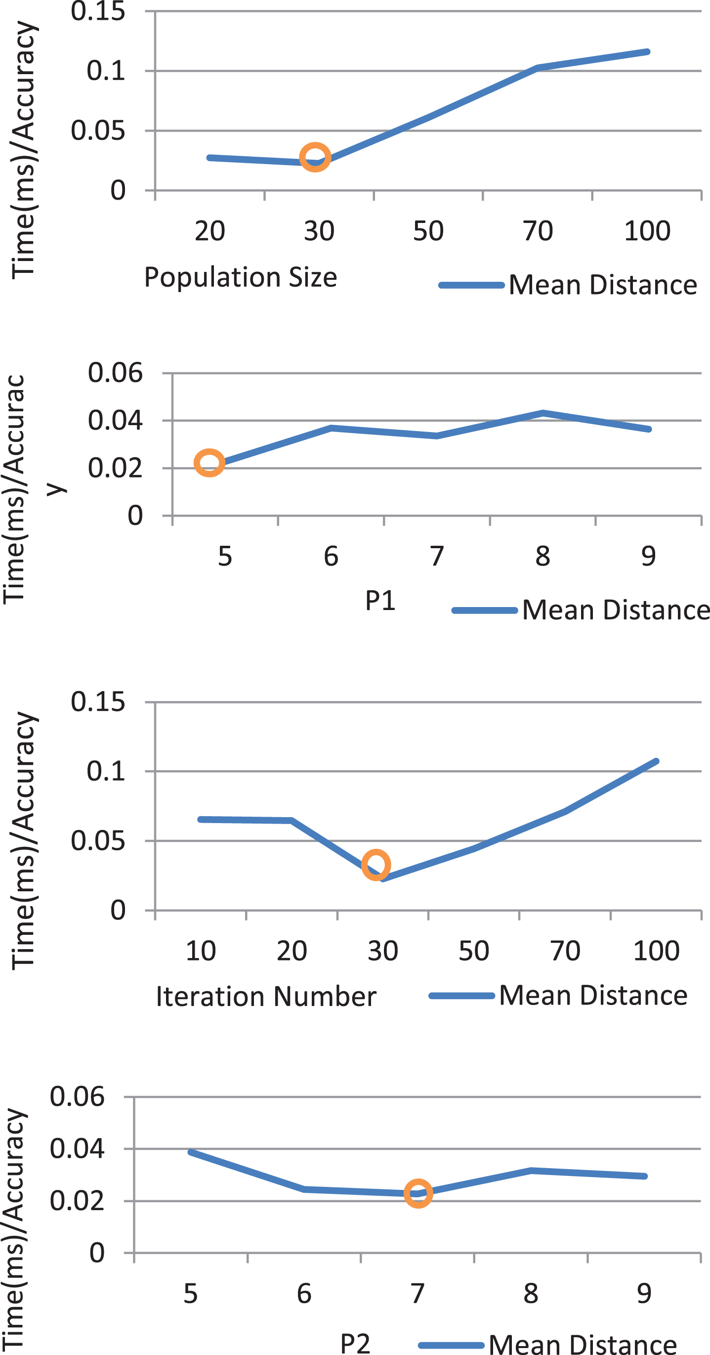
Effect of Genetic Algorithm’s Parameters on Efficiency in contrast to the Time Consumption.

2.3 Symmetry-pairs estimation

I assume symmetric pixels in each axial slice have similar intensity values, and therefore the cluster of each one should be influenced by the other one. There are two limitations impacting this assumption: first, how to determine the symmetrical pairs, since reflection of the extracted MSS on each frame is a curve, not a symmetry axis; second, two estimated symmetry pairs are not completely match.

To overcome the first limitation, I introduced an automatic symmetric pair estimation method based on the extracted MSS (Fig. 7). Figure 7(a) shows the estimated symmetry curve in a number of frames on two sagittal and coronal views and Fig. 7(b) illustrates the applied method. In this figure, A is an arbitrary pixel in a 2D axial frame. This process determines its corresponding symmetric pair, A^′, according to the symmetry cure, C. 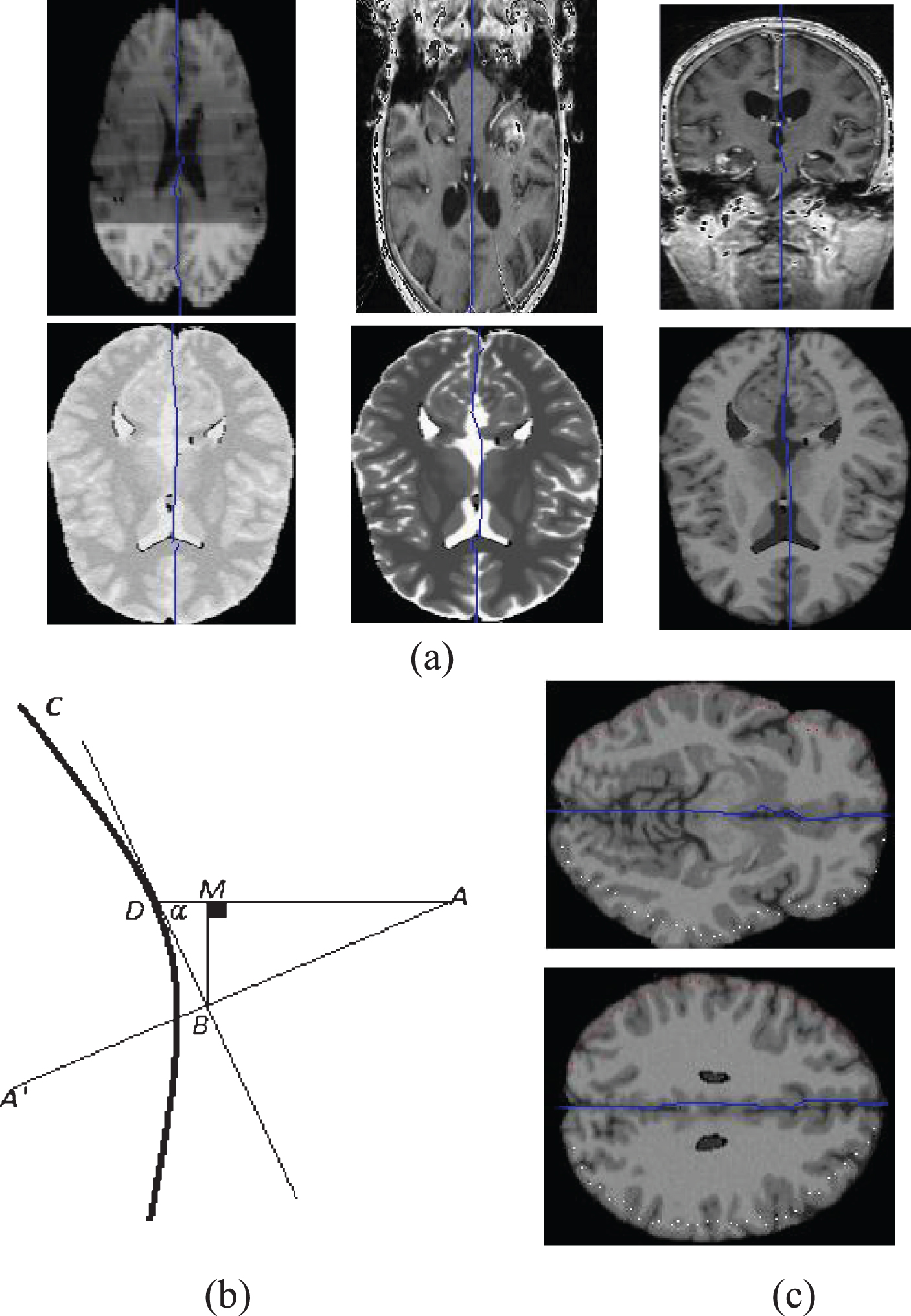In the ideal state, C is orthogonal to the horizontal line crossing from A and its mirror pixel, which is located in $2 \times D - \bar{AD}$ . But in an exaggerated sample, C makes an angle, α, with $\bar{AD}$ and moves the conjunction point for $\bar{MB}$ vertically, so that the coordinates of A^′ are $(2 \times B - \bar{AB}, 2 \times B - \bar{BM})$ . α is calculated based on two immediate neighbor pixels in two sides of point D, and $\bar{BM}$ is calculated according to the following formula. In practice, and in order to calculate $\bar{AB}$ , B is substituted with the corresponding pixel value at the same level on the curve.

Fig. 7

How to determine symmetric pairs? (a) Number of estimated MSS samples. (b) Method to detect symmetrical pairs for an arbitrary pixel in a 2D frame. (c) Two sample images and the corresponding estimated symmetrical pairs.

$\bar{MB} = \frac{sin (2 \times α) \times \bar{AD}}{2}$ (16)

Figure 7(c) shows a number of pixels and their corresponding estimated symmetric pairs in two sides of the MSS.

I use spatial information to overcome the second limitation and to increase the adaptability between symmetric pairs. Let $ℵ_{\underline{A^{'}}}$ denotes a chosen 2D local neighborhood configuration. Among A′, the estimated pair for A, and the considered neighbourhood, $ℵ_{\underline{A^{'}}}$ , the nearest pixel to A′ with the minimum difference value with A is selected as the estimated pair of A.

2.4 Applying symmetry information to SPFCM

So far I have specified the symmetric pair of each pixel in the image. The ideal is that each pair voxels have similar values and classes. In this step I use this principle to increase the accuracy of the SPFCM. The algorithm first computes symmetry measure for each pair (this parameter shows the similarity and the reliability of a pixel and its estimated pair). Several methods have been introduced in [29] to calculate the symmetry measure.

Here, I introduce a new method based on the fact that symmetrical pairs and their neighbors tend to have similar textures and intensity values. Contrary to others who only use intensity values, my symmetry measure is based on both textural information and intensity values. This definition immunizes the symmetry measure confront of the noisy pixels.

The proposed method calculates Local Binary Pattern [30] for each pixel to detect the differences between symmetric pixels. Symmetrical pairs are expected to have minimum texture difference.

${LBP}_{\underline{ρ}} = \sum_{i = 1}^{N} f (p_{i} - p_{c}) \times 2^{s}$ (17) $f (p_{i} - p_{c}) = {\begin{matrix} 1 p_{i} ⩾ p_{c} \\ 0 otherwise \end{matrix}$ (18) where p_c and p_i stand for grey values of the central pixel $(\underline{ρ})$ and each N neighbouring pixels (N = 8), respectively. The function f (.) is defined as equation (18). LBP is 0 when the central pixel has a value exactly equal to its neighbors, and is 256 when they are completely different. I assigned s with a constant value (s=5) because of meaninglessness of direction of changes among different neighbors. Using a normalization equation and the difference between each double LBP values, the first part of the proposed symmetry measure is calculated as follows. $β_{\underline{ρ}}^{1} = \frac{1}{1 + e^{- ({DLBP}_{\underline{ρ}} - μ) / δ}}$ (19) ${DLBP}_{\underline{ρ}} = | {dLBP}_{\underline{ρ}} - {dLBP}_{\underline{ρ^{'}}} |$ (20) ${dLBP}_{\underline{ρ}} = \frac{1}{| ℵ_{\underline{ρ}} |} \sum_{\underline{y} \in ℵ_{\underline{ρ}}} [λ_{\underline{ρ}} \times {LBP}_{\underline{ρ}} + (1 - λ_{\underline{ρ}}) \times {LBP}_{\underline{y}}]$ (21) where $β_{\underline{ρ}}^{1}$ denotes symmetry measure based on the texture information. ${DLBP}_{\underline{ρ}}$ measures the dissimilarity between LBP values and their mirrors. ℵ is a neighbourhood of the MR signal, $| ℵ_{\underline{ρ}} |$ is cardinality of ℵ, and $λ_{\underline{ρ}}$ is the weighting factor which controls the influence degree of the neighboring voxels $s (\underline{y}) \in ℵ_{\underline{ρ}}$ on the centroid $s (\underline{ρ})$ . $λ_{\underline{ρ}}$ is defined as equation (10). μ and δ are the mean and the standard deviation of intensity values in the image, respectively.

Two symmetric pixels with similar textures may not have the same intensities. Here, the difference between intensity values of each pixel and its neighborhoods with the corresponding intensity value of the mirror pixel and its neighborhoods is calculated and multiplied by the calculated symmetry degree. $β_{\underline{ρ}} = (1 - \frac{| d_{\underline{ρ}} - d_{\underline{ρ^{'}}} |}{d_{\underline{ρ}} + d_{\underline{ρ^{'}}}}) \times β_{\underline{ρ}}^{1}$ (22) $d_{\underline{ρ}} = \frac{1}{| ℵ_{\underline{ρ}} |} \sum_{\underline{y} \in ℵ_{\underline{ρ}}} [s (\underline{ρ}) λ_{\underline{ρ}} + s (\underline{y}) (1 - λ_{\underline{ρ}})]$ (23) where $β_{\underline{ρ}}$ defines the degree of symmetry for $\underline{ρ}$ and its mirror, $\underline{ρ^{'}}$ . $β_{\underline{ρ}}$ can vary from 0 (totally asymmetric) to 1 (perfectly symmetrical).

In the conventional FCM and in its derived versions such as SPFCM, the pixels are allocated to different classes according to the distance between their intensity values and centroids of the clusters, so that when a pixel is far from a centroid, it has less chance of belonging to that class. In this research, I add distances between the mirror pixels and the centroids to the distance of the pixels and the corresponding centroids. For this purpose, I introduce a weighting parameter, which weights the symmetric pair distances with each centroid. ${\begin{matrix} α (β_{\underline{ρ}}) = β_{\underline{ρ}} if β_{\underline{ρ}} ⩾ θ \\ 0 otherwise \end{matrix}$ (24)

By setting a threshold value to $β_{\underline{ρ}}$ , I suppress the symmetry if $β_{\underline{ρ}} < θ$ . The value of θ is set to 0.6 experimentally.

After applying the symmetry information I calculate the objective function for the GSPFCM clustering algorithm by $\begin{matrix} J_{GASPFCM} = \sum_{\underline{ρ} \in I} \sum_{k = 1}^{c} ({au}_{k, \underline{ρ}}^{m} + a^{,} t_{k, \underline{ρ}}^{n}) \\ \frac{D_{k, \underline{ρ}} + α (β_{\underline{ρ}}) \times D_{k \underline{, ρ^{,}}}}{α (β_{\underline{ρ}}) + 1} + \sum_{k = 1}^{c} η_{k} \sum_{\underline{ρ} \in I} {(1 - t_{k, \underline{ρ}})}^{n} \\ + β η (w_{z} (ρ, y)) + γ φ (w_{z} (ρ, y)) \end{matrix}$ (25) subject to the constraints $0 ⩽ u_{k, \underline{ρ}}^{m}, t_{k, \underline{ρ}}^{n} ⩽ 1, \sum_{\underline{ρ} \in I} t_{k, \underline{ρ}} = 1 \forall k$ , and $\sum_{k = 1}^{c} u_{k, \underline{ρ}} = 1 \forall \underline{ρ} \in I$ , where $t_{k, \underline{ρ}}$ refers to the probabilistic value of $s (\underline{ρ})$ in the kth cluster, c_k. $D_{k, \underline{ρ}}$ and $D_{k, \underline{, ρ^{,}}}$ measure the dissimilarity between c_k and the captured MR signal at pixels $\underline{ρ}$ and $\underline{ρ^{,}}$ respectively. η (w_z (ρ, y)) and φ (w_z (ρ, y)) are defined as equations (6) and (7) respectively. $α (β_{\underline{ρ}})$ is the weighting parameter between symmetric pairs. The necessary conditions for minimization of J_GSPFCM over the memberships $u_{k, \underline{ρ}}$ , the possibilistic values $t_{k, \underline{ρ}}$ , and cluster centroids v_k are obtained by setting the respective first partial derivatives of J_GSPFCMto zero, while keeping the other variables constant. Considering Lagrange functional, differentiating with respect to $u_{k, \underline{ρ}}$ , $t_{k, \underline{ρ}}$ and v_k, respectively, and setting the results to zero yields: $u_{k, \underline{ρ}} = {[\sum_{l = 1}^{c} {(\frac{D_{k, \underline{ρ}} + α (β_{\underline{ρ}}) \times D_{k, \underline{ρ^{'}}}}{D_{l, \underline{ρ}} + α (β_{\underline{ρ}}) \times D_{l, \underline{ρ^{'}}}})}^{2 / m - 1}]}^{- 1}$ (26) $t_{k, \underline{x}} = \frac{1}{1 + {(b \times \frac{D_{k, \underline{ρ}} + α (β_{\underline{ρ}}) \times D_{k, \underline{ρ^{'}}}}{η_{k}})}^{\frac{1}{n - 1}}}$ (27) ${\begin{matrix} α (β_{\underline{ρ}}) = β_{\underline{ρ}} if β_{\underline{ρ}} ⩾ θ \\ 0 otherwise \end{matrix}$ (28) $g_{\underline{ρ}}$ and $g_{{\underline{ρ}}^{'}}$ are calculated using Equation (14).

3 MR brain image segmentation

The method was implemented using C++ in the MS Visual Studio environment and were tested on both simulated and real 3D MR images. Simulated brain data with different noise and INU levels and their ground truths were obtained from the BrainWeb Simulated Brain database at the McConnell Brain Imaging Centre of the Montreal Neurological Institute (MNI), McGill University [31], and the real MRI data were obtained from the Internet Brain Segmentation Repository (IBSR), Massachusetts General Hospital [32]. Extra-cranial tissues were removed from all images prior to segmentation. The number of tissue classes in the segmentation was set to three, which correspond to Grey Matter (GM), White Matter (WM) and Cerebrospinal Fluid (CSF). Background pixels were ignored in the computation. For the simulated 3D MRI brain images, the dimensions were 217 × 181 × 181 [row (y) × column (x) × depth (z)], and for the real 3D MRI brain images, these values were [55–61]×265×265. The algorithms were run on a Pentium i5 3.2-GHz 4 G PC.

3.1 Parameter setting

The first four results in Table 2 demonstrate that if I vary a^, from 1 to 10, keeping all other parameters fixed, the best results are achieved when a^, = 7. However, the changes are not a lot. It is because, increasing a^, when the value of a is fixed, assigns more importance to typicality. The results do not change much since, in the simulated images, there are a number of nice-well separated clusters so that their segmentation is done well by membership concept of GSPFCM. However, if the data have outliers, giving more importance to typicality by increasing a^,, improves the prototypes. Generally, this property can be used to get a better understanding of the data [33]. When I discuss the values of a and a^,, a natural question comes: should I constraint these parameters to a + a^, = 1 ? Acceptation of this constraint means that if I increase the importance of one (for example membership vale) it necessarily forces me to reduce the importance of the other one (for example typicality) which is too restrictive. In order to investigate this matter experimentally, I conducted tests in rows 6 and 7. The results show a considerable drop in results. In the rows 7 to 10, I evaluated the results when the values of m and n are changed and the values of two first coefficients are fixed. The changes were done in two states when m is much more that n and when n is much bigger than m. These values mean the effect of one factor, typicality via membership values, dramatically changes. The results showed that in both states the error rate increases and the best results are achieved with similar values for m and n. Because the more acceptable results with lower values for m and n parameters in the first rows compared to the recent evaluated rows (rows 7 to 10), it is concluded that the best results are achievable with low similar values for these two parameters. Finally the two last rows of the table show that the best value for m and n is 2. As a result, I assigned a, a^,, m, and n parameters with 1, 7, 2, and 2 respectively.

Table 2
Results produced by GSPFCM for different values of the parameters

a a ^, m N MCR WM GM CSF GM+WM

1 1 1 2 2 3.64 96.63 95.38 90.16 98.97

2 1 5 2 2 3.47 96.64 95.60 90.21 99.00

3 1 7 2 2 3.46 96.64 95.62 90.27 99.00

4 1 10 2 2 3.45 96.64 95.63 90.18 99.00

5 0.5 0.5 2 2 3.86 96.58 95.06 89.56 98.93

6 0.125 0.875 2 2 3.83 96.55 95.12 88.62 98.93

7 1 7 5 1.5 9.33 94.17 88.64 73.59 97.72

8 1 7 5 5 5.67 95.60 92.90 84.50 98.36

9 1 7 5 8 4.22 96.30 94.73 86.70 98.82

10 1 7 5 10 4.32 96.12 94.66 85.08 98.80

11 1 7 2 3 3.60 96.66 95.46 89.96 98.98

12 1 7 3 3 5.03 96.00 93.75 84.01 98.67

	a	a ^,	m	N	MCR	WM	GM	CSF	GM+WM
1	1	1	2	2	3.64	96.63	95.38	90.16	98.97
2	1	5	2	2	3.47	96.64	95.60	90.21	99.00
3	1	7	2	2	3.46	96.64	95.62	90.27	99.00
4	1	10	2	2	3.45	96.64	95.63	90.18	99.00
5	0.5	0.5	2	2	3.86	96.58	95.06	89.56	98.93
6	0.125	0.875	2	2	3.83	96.55	95.12	88.62	98.93
7	1	7	5	1.5	9.33	94.17	88.64	73.59	97.72
8	1	7	5	5	5.67	95.60	92.90	84.50	98.36
9	1	7	5	8	4.22	96.30	94.73	86.70	98.82
10	1	7	5	10	4.32	96.12	94.66	85.08	98.80
11	1	7	2	3	3.60	96.66	95.46	89.96	98.98
12	1	7	3	3	5.03	96.00	93.75	84.01	98.67

3.2 Time complexity of the GSPFCM

The time complexity of GSPFCM is not much more than the other segmentation methods. Generally adding a number of information terms to objective function of GSPFCM increases its time consumption. However, the time complexity of this method is not much more than the other methods. Let’s have a look in details. The time complexity of GSPFCM equals to maximum complexity of triple phases of the proposed method; MSS extraction, Symmetry-pairs estimation, and applying symmetry information to SPFCM. For the MSS extraction, unlike this fact that naturally evolutionary algorithms are slow, the algorithm looks for a proper fitting set of pixels inside a limited area around the extracted MSP; I hope the genetic algorithm converges soon, so that in average total time complexity of the MSS extraction method is a ratio of the image slice number. In order to estimate symmetry-pair of each pixel in different slides, a sequence of calculations is done. As a result, time order of symmetry pair estimation for each pixel is o(1) and the total time complexity of the symmetry pair estimation algorithm is a ration of size of the picture. Finally, adding a number of terms to objective function of GSPFCM and the updating formulas increases time consumption of the method, but it does not have effect on the time complexity. As a result, I claim that time complexity of GSPFCM is not much more than other segmentation methods such as ASFCM, FCM, PFCM and so.

3.3 Visual performance of the MSS extraction method

In this experiment, a comprehensive qualitative experiment was conducted in the hope to show performance of the proposed method in extracting MSS under different conditions. For this purpose, both normal and pathological MR images from IBSR were used. Figure 8 presents a number of the results projected on the axial or coronal slices. Two first images of the first row show the output of a normal T1 MRI in the axial view and the next two images present the output in the coronal view. The second row illustrates effectiveness of the algorithm on the normal brain images captured under different INU conditions. The third row is belonged to T2 modality images while the fourth row shows the extracted MSSs for Parkinson’s Disease (PD) modality images. Finally, effectiveness of the algorithm on pathological images is highlighted in the last row images.

Fig. 8

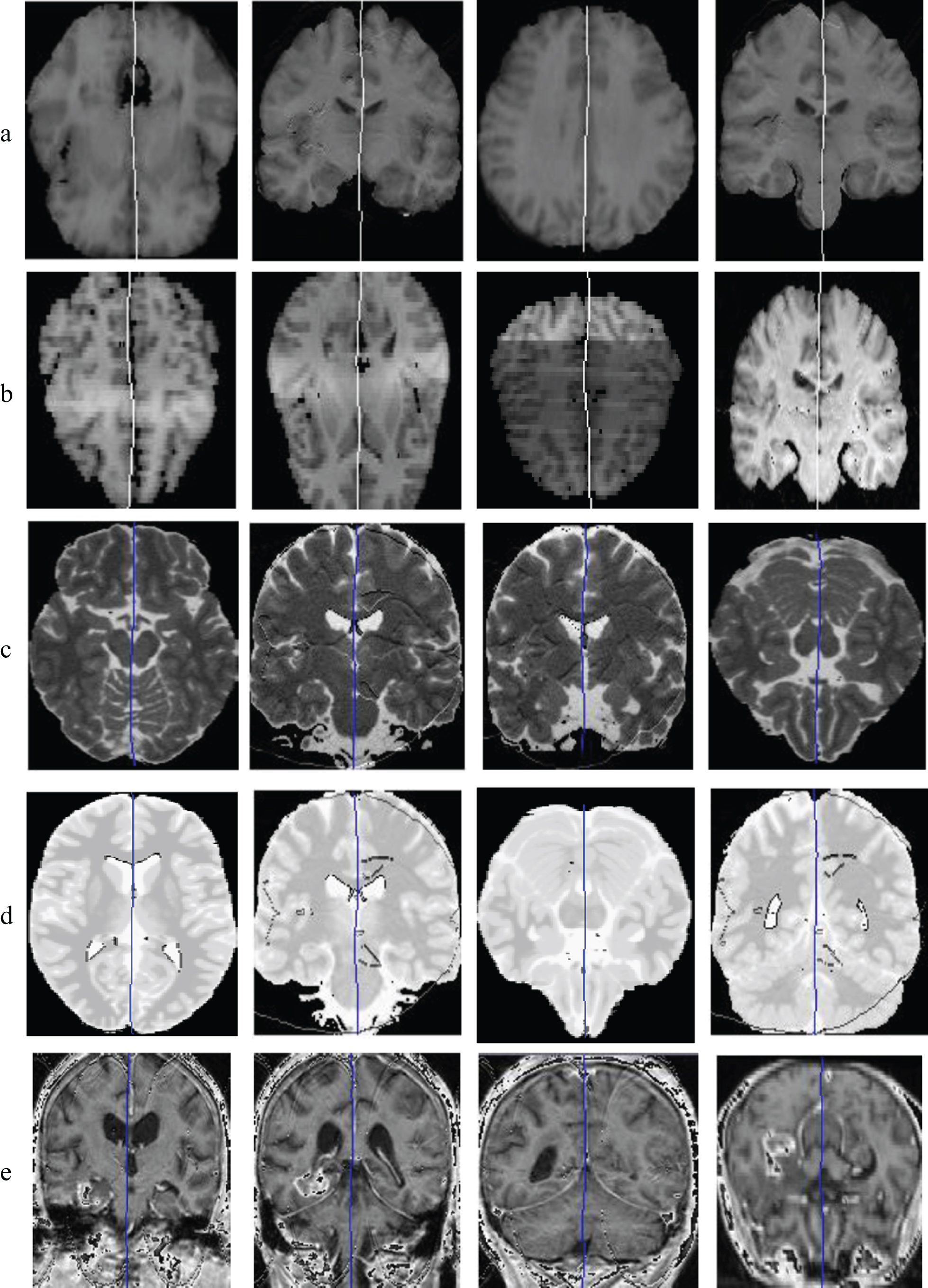
Estimated MSSs by the genetic algorithm projected at axial/coronal slices. a: Images at different axial locations and different coronal slices. b: Normal brain images captured under different INU conditions. c: T2 modality. d: PD modality. e: Pathological images.

In addition, the effect of noise, INU, slice thickness, and modality on the visual quality of the estimated MSS was investigated using the simulated images from BrainWeb dataset. The results are shown in Fig. 9. As it is shown in this image, the proposed algorithm is robust in facing various amounts of these effects.

Fig. 9

Effect of different levels of noise, INU, and modality on the performance of the estimated MSS by the genetic algorithm.

3.4 GSPFCM visual performance on simulated images

Figure 10 shows a number of simulated MRI brain images, taken at different slices. The image of Fig. 10(1a) has been simulated from the true model with the following settings: modality, ICBM protocol [34], slice thickness of 1 mm (1 voxels), 3% noise level and 40% INU. Figure 10(1b) was generated based on a discrete anatomical normal brain model and serves as the true model. Figure 10(1c) shows the actual bias field producing the INU artefact. Figure 10(1d) shows the segmented image, and Fig. 10(1e) presents the recovered bias field, which resembles very closely the actual bias field of Fig. 10(1c). The next two rows in Fig. 10 illustrate the same information for slices taken near to the base of the brain (z = 39) and near to the top of the skull (z = 140), respectively.

Fig. 10

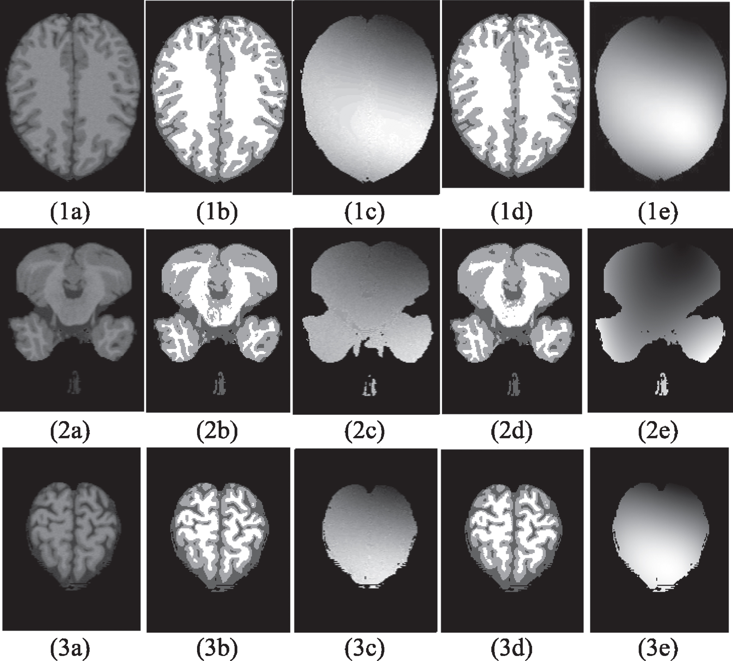
Segmentation Results by the GSPFCM for the Simulated MRI Slices. From Left to Right: Image Corrupted with Noise and INU Artefact, True Model, The Corresponding Bias Field, The Segmentation Result, and the Recovered Bias Field. From Top to Bottom: z = 110, z = 39, and z = 140.

3.5 Visual performance of GSPFCM for real images

To show the outcomes of the proposed segmentation method on real images, the following experiment was carried out. Figure 11 presents a slice (z = 36) of the IBSR 8 bit T1 Normal brain 6_10 image. In this figure, CSF, GM, and WM are shown in Fig. 11(1b), (1c), and (1d), respectively. The same images are shown in the next two rows for slices taken near to the back of the brain (z = 12) and near to the front of the skull (z = 45), respectively. Please note that in real MR data, images are scanned slice by slice in the sagittal direction.

Fig. 11

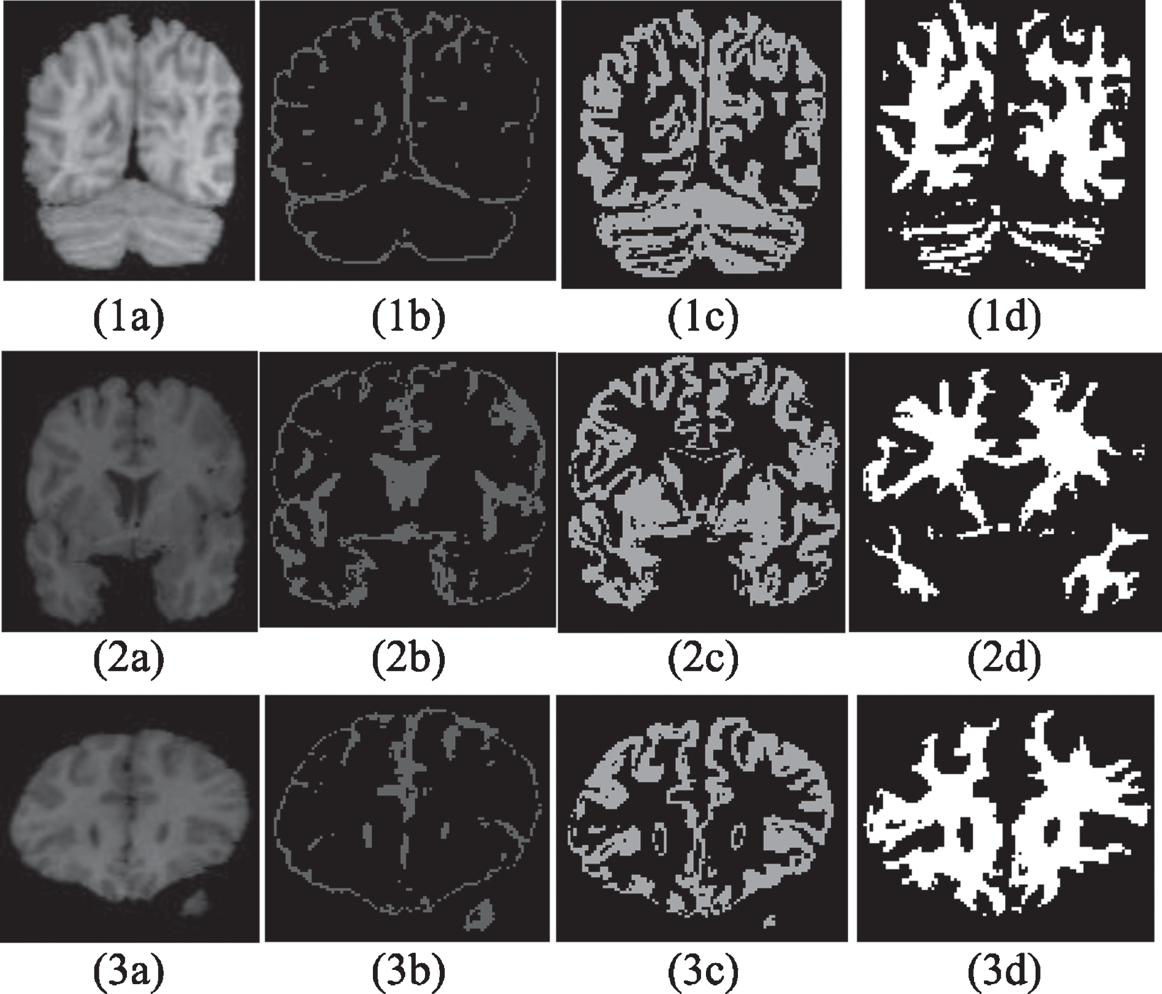
Segmentation Results for a Real Image (a) Slice Image, Segmentation Results show GM(a), CSF (b), and WM(c), (1) z = 36. (2) z = 12, (3) z = 45.

3.6 Quantitative evaluation

For comparison, I calculated the MCR value of a number of re-implemented segmentation methods, namely, ASFCM (Adaptive Spatial FCM) [26], SymFCM (Symmetry FCM) [4], FCM (Fuzzy C-Mean Classification) [24], MRF (Markov Random Field) [35], EM (Expectation Maximization) [36], and PCM (Possibilistic C-Mean) [11], FPCM (Fuzzy PCM) [10], and PFCM (Possibilistic FCM) [11] as the state-of-the-art methods in possibilistic methods. Simulated MRI data was used with weighted T₁ voxels, 3% noise, 40% level of INU inhomogeneity and slice thickness of 1 mm. Table 3 shows that the GSPFCM had better performance compared to the other methods. Each column in this table shows the average result for all slices (all 145 non-empty slices from 217 ones).

Table 3
Comparison of the ASFCM, SymFCM, FCM, MRF, EM, PCM, FPCM, and PFCM algorithms in terms of Overlap Metric (IN %) for different tissue classes, and the MCR (IN %), for the simulated image with INU = 40%

GSPFCM ASFCM SymFCM FCM MRF EM PCM FPCM PFCM

MCR(%) 3.54 3.76 9.52 9.61 9.61 11.47 12.54 9.61 9.61

WM 96.64 96.66 95.04 94.22 94.22 92.21 92.89 94.22 94.22

GM 95.54 95.28 87.90 87.89 87.98 86.93 82.43 87.89 87.89

CSF 90.22 88.93 77.12 74.32 74.32 69.45 76.15 74.32 74.32

GM+WM 99.00 98.35 97.34 97.33 97.33 95.44 96.00 97.33 97.33

	GSPFCM	ASFCM	SymFCM	FCM	MRF	EM	PCM	FPCM	PFCM
MCR(%)	3.54	3.76	9.52	9.61	9.61	11.47	12.54	9.61	9.61
WM	96.64	96.66	95.04	94.22	94.22	92.21	92.89	94.22	94.22
GM	95.54	95.28	87.90	87.89	87.98	86.93	82.43	87.89	87.89
CSF	90.22	88.93	77.12	74.32	74.32	69.45	76.15	74.32	74.32
GM+WM	99.00	98.35	97.34	97.33	97.33	95.44	96.00	97.33	97.33

A paired t-test was performed to reveal the reliable difference between the mean MCR value of my method and that of the other six methods. The comparison results with these methods for the probability value for a 95% confidence level are shown in Table 4. In these tests, all 145 2D simulated frames participated.

Table 4

Results of the paired t-test in the simulated images

with ASFCM	with SymFCM	with FCM	with MRF	with EM	with PCM	with FPCM	With PFCM
–8.785	–5.935	–7.037	–7.101	–6.772	–12.325	–8.970	–6.104

To show the enhancement of GSPFCM compared to all the segmentation methods used in the last test plus ASFCM [26], a more comprehensive experiment, the quantitative measures were calculated for 573 2D axial slices. The average values and the standard deviation values for the factors through different slices are plotted in Figs. 12 and 13. Overall, the charts show the enhancement of GSPFCM compared to the others.

Fig. 12

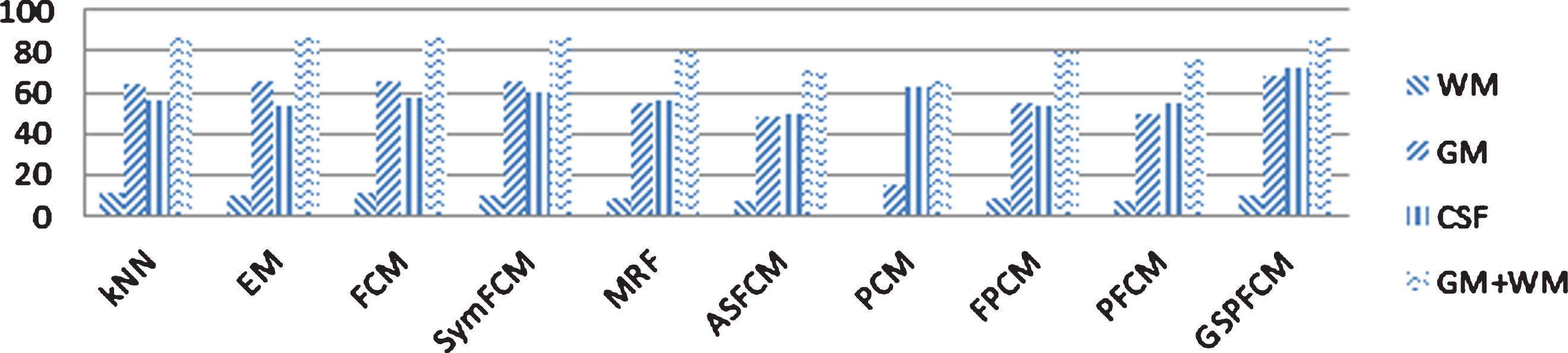
Average Quantitative Measures through 573 Real Images.

Fig. 13

Standard Deviation Quantitative Measures through 573 Real Images.

Table 5 illustrates the average values between all these slices for each of the segmentation algorithms.

Table 5

Comparison of GASPFCM, ASFCM, FCM, MRF, EM, FPCM, and PFCM algorithms in terms of Overlap Metric (IN %) for different tissue lasses, and the MCR (IN %), for real images

	GA SPFCM	ASFCM	SymFCM	FCM	MRF	EM	FPCM	PFCM
WM	13.32	6.37	10.99	10.99	6.50	13.77	6.24	6.24
GM	71.97	31.45	48.16	47.38	33.39	56.34	32.12	31.82
CSF	73.92	11.04	23.76	22.20	10.11	10.62	11.05	10.98
GM+WM	89.54	71.84	87.39	85.49	73.58	85.94	72.23	72.23
MCR(%)	31.41	75.59	57.12	60.06	74.25	54.17	75.20	75.388

Like the simulated images, a paired t-test was performed between the mean MCR values of my method and those of the other four methods. Comparison results with a 95% confidence level are shown in Table 6. These results indicate that I have a statistically significant lower mean value. There are 573 2D images in this test.

Table 6

Results of the paired t-test in real images

with ASFCM	with SymFCM	with MRF	with kNN	with EM	with FCM	with PCM	with FPCM	with PFCM
–17.631	–8.547	–16.582	–10.401	–9.302	–9.787	–25.591	–16.220	–20.671

4 Conclusion

In this paper, I introduced a new version of Fuzzy C-Mean classifier named GSPFCM. In GSPFCM, symmetry information was integrated into SPFCM. SPFCM is a new version of PFCM, including possibilistic and spatial information. Briefly, first I added the possiblistic and spatial information to FCM via a new objective function for SPFCM. Then, I estimated the Mid-Sagittal Surface and determined symmetric pairs on two sides of the MSS. For each pair, I calculated a symmetry degree. A new objective function was introduced and the updating formulas of the cluster’s centroids and the membership values were modified. As a result, I had a classifier method which used membership information, possibilistic information, spatial information, and symmetry information. The comprehensive tests using two standard real and simulated datasets showed the effectiveness of GSPFCM. In the simulated images, where the accuracy is more, GSPFCM reached to 99 percent which was more than all the compared methods. In real images, segmentation accuracy is dependent on the quality of the images. However, in all the applied images, GSPFCM achieved a better result. In the best condition, I got 89.54 percentage, and in average, the results were about 5 percent better than the other methods.

Conflicts of interest

I, Seyed Hashem Davarpanah, certify that I have participated sufficiently in the work to take public responsibility for the content, including participation in the concept, design, analysis, writing, or revision of the manuscript. Furthermore, I certify that this material has not been and will not be submitted to or published in any other publication. I also certify that I have NO affiliations with or involvement in any organization or entity with any financial interest, or non-financial interest in the subject matter or materials discussed in this manuscript.

References

Jayasuriya

S.A.

, Liew

A.W.C.

and Law

N.F.

, Brain symmetry plane detection based on fractal analysis, Computerized Medical Imaging and Graphics 37(2013), 568–580.

Kuijf

H.J.

, van Veluw

S.J.

, Geerlings

M.I.

, Viergever

M.A.

, Biessels

G.J.

and Vincken

K.L.

, Automatic extraction of the midsagittal surface from brain MR Images using the Kullback-Leibler measure, Neuroinformatics 12 (2014), 395–403.

Ortiz

, Palacio

A.A.

, Gorriz

J.M.

, Ramirez

and Salas-Gonzalez

, Segmentation of Brain MRI Using SOM-FCM-Based Method and 3D Statistical Descriptors, Computational and Mathematical Methods in Medicine 2013 (2013), 12.

Jayasuriya

S.A.

and Liew

A.C.

, Symmetry incorporated fuzzy c-means method for image segmentation, in Fuzzy Systems (FUZZ), 2013 IEEE International Conference on, 2013, pp. 1–7.

Yang

and Huang

, Image Segmentation by Fuzzy C-Means Clustering Algorithm with a Novel Penalty Term, Computing and Informatics 26 (2007), 17–31.

Lou

, Li

and Liu

, Improved Fuzzy C-means Clustering Algorithm Based on Cluster Density, Journal of Computational Information Systems 8 (2012), 727–737.

Cai

, Chen

and Zhang

, Fast and robust fuzzy c-means clustering algorithms incorporating local information for image segmentation, Pattern Recognition 40 (2007), 825–838.

Liu

Z.-G.

, DezertJ. Gr, #233, , Mercier

and Pan

, Belief C-Means: An extension of Fuzzy C-Means algorithm in belief functions framework, Pattern Recogn Lett 33 (2012), 291–300.

Krishnapuram

and Keller

J.M.

, The possibilistic C-means algorithm: insights and recommendations, Fuzzy Systems, IEEE Transactions on 4 (1996), 385–393.

10.

Pal

N.R.

, Pal

and Bezdek

J.C.

, A mixed c-means clustering model, in, Fuzzy Systems, 1997, Proceedings of the Sixth IEEE International Conference on 1 (1997), 11–21.

11.

Krishnapuram

and Keller

J.M.

, A possibilistic approach to clustering, Fuzzy Systems, IEEE Transactions on 1 (1993), 98–110.

12.

Liu

S.X.

, Symmetry and asymmetry analysis and its implications to computer-aided diagnosis: A review of the literature, Journal of Biomedical Informatics 42 (2009), 1056–1064.

13.

and Bhanu

, Reflection Symmetry-Integrated Image Segmentation, Pattern Analysis and Machine Intelligence, IEEE Transactions on 34 (2012), 1827–1841.

14.

Cicconi

and Kunt

, Symmetry-based image segmentation, 1993, pp. 378–384.

15.

Tyng-Luh

, Geiger

and Yuille

A.L.

, Segmenting by seeking the symmetry axis, in Pattern Recognition, 1998. Proceedings. Fourteenth International Conference on, 1998, pp. 994–998, vol. 2.

16.

Shor

and Kiryati

, Towards Segmentation from Multiple Cues: Symmetry and Color, in Multi-Image Analysis. vol. 2032, R. Klette, G. Gimel’farb, and T. Huang, Eds., ed: Springer Berlin Heidelberg, 2001, pp. 142–152.

17.

Gupta

, Prasad

V.S.N.

and Davis

L.S.

, Extracting Regions of Symmetry, in International Conference on Image Processing, 2005, pp. 133–136.

18.

Riklin-Raviv

, Kiryati

and Sochen

, Segmentation by Level Sets and Symmetry, in Computer Vision and Pattern Recognition, 2006 IEEE Computer Society Conference on, 2006, pp. 1015–1022.

19.

Jiao

, Fu

and Bi

, Brain Image Segmentation Based on Bilateral Symmetry Information, in Bioinformatics and Biomedical Engineering, 2008. ICBBE 2008. The 2nd International Conference on, 2008, pp. 1951–1954.

20.

, Bhanu

and Bhanu

, Automatic symmetry-integrated brain injury detection in MRI sequences, in Computer Vision and Pattern RecognitionWorkshops, 2009. CVPR Workshops 2009. IEEE Computer Society Conference on, 2009, pp. 79–86.

21.

Khotanlou

, Colliot

, Atif

and Bloch

, 3D brain tumor segmentation in MRI using fuzzy classification, symmetry analysis and spatially constrained deformable models, Fuzzy Sets and Systems 160 (2009), 1457–1473.

22.

Saha

and Bandyopadhyay

, MRI brain image segmentation by fuzzy symmetry based genetic clustering technique, in Evolutionary Computation, 2007. CEC 2007. IEEE Congress on, 2007, pp. 4417–4424.

23.

Kuijf

, Viergever

and Vincken

, Automatic Extraction of the Curved Midsagittal Brain Surface onMRImages, in Medical Computer Vision. Recognition Techniques and Applications in Medical Imaging. vol. 7766, B. Menze, G. Langs, L. Lu, A. Montillo, Z. Tu, and A. Criminisi, Eds., ed: Springer Berlin Heidelberg, 2013, pp. 225–232.

24.

Bezdek

J.C.

, Pattern Recognition with Fuzzy Objective Function Algorithms: Kluwer Academic Publishers, 1981.

25.

Davarpanah

S.H.

and Liew

A.W.-C.

, Spatial Possibilistic Fuzzy C-Mean Segmentation Algorithm Integrated with Brain Mid-sagittal Surface Information, International Journal of Fuzzy Systems 19 (2017), 591–605.

26.

Liew

A.W.C.

and Hong

, An adaptive spatial fuzzy clustering algorithm for 3-D MR image segmentation, Medical Imaging, IEEE Transactions on 22 (2003), 1063–1075.

27.

Davarpanah

S.H.

and Liew

A.W.-C.

, Brain Mid-sagittal Surface Extraction Based on Fractal Analysis, Neural Computing and Applications 30 (2018), 153–162.

28.

Stegmann

M.B.

, Skoglund

and Ryberg

, Mid-sagittal plane and mid-sagittal surface optimization in brain MRI using a local symmetry measure, in SPIE, 2005, 568–579.

29.

O’Mara

and Owens

, Measuring bilateral symmetry in digital images, in TENCON ’96. Proceedings, 1996 IEEE TENCON. Digital Signal Processing Applications 1 (1996), 151–156.

30.

Davarpanah

S.H.

, Khalid

, Nurliyana Abdullah

and Golchin

, A texture descriptor: BackGround Local Binary Pattern (BGLBP), Multimedia Tools and Applications, 1–20, 2015.

31.

Kwan

R.K.S.

, Evans

A.C.

and Pike

G.B.

, MRI simulation-based evaluation of image-processing and classification methods, Medical Imaging, IEEE Transactions on 18 (1999), 1085–1097.

32.

IBSR. Center for Morphometric Analysis Internet Brain Segmentation Repository (IBSR), Massachusetts General Hospital [Online].

33.

Pal

N.R.

, Pal

, Keller

J.M.

and Bezdek

J.C.

, A Possibilistic Fuzzy c-Means Clustering Algorithm, IEEE Transactions on Fuzzy Systems 13 (2005), 517–530.

34.

I.C.B.M.I. Univ. California, Lab. Neuro Imag, Quebec, ON, Canada., Los Angeles, CA. [Online].

35.

Kato

and Pong

T.-C.

, A Markov random field image segmentation model for color textured images, Image and Vision Computing 24 (2006), 1103–1114.

36.

Altman

N.S.

, An Introduction to Kernel and Nearest-Neighbor Nonparametric Regression, The American Statistician 46 (1992), 175–185.