
Abstract
Algebraic operations are used effectively in decision-making problems. Especially, Dombi, Hamacher and Einstein algebraic operators are used frequently in the decision-making field. On the other hand, it is known that aggregation operators affect the decision-making process in decision-making problems. In this paper, we used Dombi operations to develop some Fermatean fuzzy aggregation operators. Arithmetic and geometric analysis of each aggregation method were performed. We defined the following operators: Fermatean fuzzy Dombi weighted average operator, Fermatean fuzzy Dombi weighted geometric operator, Fermatean fuzzy Dombi ordered weighted average operator, Fermatean fuzzy Dombi ordered weighted geometric operator, Fermatean fuzzy Dombi hybrid weighted average operator, Fermatean fuzzy Dombi hybrid weighted geometric operator. Also, an analysis was performed for the beta value of the Dombi parameter. Properties of proposed operators were presented, and operators were defined on Fermatean fuzzy sets. Finally, proposed operators were compared with the existing aggregation operators. To understand the impact of the proposed operators on the decision-making process, Fermatean fuzzy TOPSIS was established.
Keywords
Introduction
Unclearness or incomplete information in many areas poses major problems. Likewise, it can be said that there is incomplete and unclear information in decision-making problems. The solution of decision-making problems depends largely on the imprecision, uncertain and incomplete information. Real numbers are insufficient to solve uncertain situations. Therefore, fuzzy sets constitute the solution in an uncertain case. Fuzzy sets are introduced by Zadeh [48]. In particular, finding the degree of membership of a value within a fuzzy set helps to solve the uncertain situation. In this sense, fuzzy sets have made progress in many fields of engineering and technology. However, the elements of classical fuzzy sets are interpreted based on only the degree of membership. So, unclearness or incomplete information in a dataset only be represented by one membership function. The generalization of the concept of the classical fuzzy set is defined by Atanassov [2]. This structure is called an intuitionistic fuzzy set (IFS).
While classical fuzzy sets are represented by the only degree of membership, IFSs are represented by two values: the degree of membership and degree of non-membership. IFSs have been used, effectively in many areas such as pattern recognition, medical diagnosis, image segmentation, fuzzy time series forecasting [11, 37]. The sum of the degree of membership and non-membership degree is defined in the unit interval. Likewise, each degree is in the [0,1] interval. When the sum of membership and non-membership values is greater than 1 then when we cannot define the IFS. For example, if both membership degrees are greater than 0.5, IFS is not provided. To generalize the IFS concept, the Pythagorean fuzzy set (PFS) was defined by Yager [46]. In PFS, the membership and non-membership degrees are in the [0,1] interval. However, the sum of squares of membership degrees varies in the unit closed interval. In this case, the PFS is larger fuzzy sets than the IFSs. Then, we can say that PFS offers more advantages than IFS in solving real-world problems. For example, pattern recognition, supplier selection, industrial accident early warning, recommender systems [14, 49].
Although PFS provides a larger set, it appears to be expandable. This can be illustrated with an example. Suppose that membership degree is 0.8 and the non-membership degree is 0.7. For IFS, 0.8+0.7 < 1 condition is not provided. Similarly, for PFS, 0 . 82 + 0 .72 > 1. The sum of membership and non-membership degrees for IFS and PFS appears to be out of unit interval. So, it is considered that defining a more general fuzzy set will be effective in solving problems. Senapati and Yager proposed Fermatean fuzzy set (FFS) [33]. FFS provides a more general perspective for fuzzy sets. In FFS, the sum of cubes of membership and non-membership degrees is in the unit interval. For example, 0.83+0.73 > 1 condition is provided in FFS. Currently, it can be said that FFS is the most extended set among fuzzy sets. So far, basic issues for fuzzy sets have been addressed. In the following part of the introduction section, FFS and aggregation operators on FFS will be examined.
Aggregation methods are widely used in multiple criteria decision making (MCDM) and PFS. Wei and Lu used power aggregation operators in decision-making problems [43]. Yager introduced ordered weighted averaging aggregation operators for MCDM [45]. Khan et al. developed an aggregation operator for multi-attribute group decision making and it is emphasized that decision-makers and attributes are at different priority levels [21]. Merigo and Casanovas presented induced aggregation operators [29]. Depending on the decision-maker’s attitude, the reorder-based provides the parametrized family of distance aggregation operators. Merigó and Casanovas introduced fuzzy generalized hybrid aggregation operators and these operators are applied in the decision-making problem [30].
Algebraic operators are used for many aggregation structures. These are Dombi, Einstein, Hamacher operators. The Dombi triangular norm(t-norm) and triangular conorm(t-conorm) operator was defined in 1982 by Dombi [12]. The main advantage of Dombi norms is that it depends on the parameter value. As the parameter value changes, the resulting norm changes. Chen and Ye [4] proposed Dombi weighted aggregation operators for single-valued neutrosophic sets and applied on investment alternatives. Shi and Ye are used Dombi aggregation operators of neutrosophic cubic sets for travel decision-making [36]. Jana et al. presented bipolar fuzzy Dombi operators for the evaluation of emerging technology commercialization with multiple-attribute decision making [15]. With the widespread application of Dombi operators on Pythagorean fuzzy sets, Khan et al. proposed Pythagorean fuzzy Dombi aggregation operators on investment decision making [20]. Wei defined aggregation method for Hamacher and delivered a comparative analysis for decision making [41]. It is seen that the TOPSIS method is applied to various fields and gives effective results. Data Envelopment Analysis (DEA) was combined with the TOPSIS method [40]. The efficiency of the end-of-life vehicle reverse logistics industry was analyzed by DEA TOPSIS. In another study, the TOPSIS method is presented for probabilistic linguistic sets in multiple attribute group decision making using entropy weights. Also, probabilistic linguistic sets with TOPSIS was applied to Supplier Selection of New Agricultural Machinery Products [27]. TOPSIS extended with the Choquet integral based method [39]. Besides, the TOPSIS-Choquet integral method was used in the interval-valued hesitant Pythagorean fuzzy environment.
In 2016, the q-rung orthopair fuzzy set was introduced by Yager [47]. Intuitionistic fuzzy sets were expanded from the qth degree. On the other hand, aggregation methods have been described on q-rung fuzzy sets [26, 44]. Also, in q-rung orthopair fuzzy sets were used Dombi operator [16]. However, this study, a comprehensive TOPSIS method for multiple decision making on Fermatean fuzzy sets is included. The distance method presented for IFSs was extended for FFSs and more accurate distance calculation was performed [19].
Senapati and Yager introduced new aggregated operators in [34]. The operators are presented with practical examples. These operators will also be included in our study. Senapati and Yager defined basic operators over the FFSs. On the other hand, division and subtraction operations on FFSs were defined in [35]. They implemented the weighted product model on MCDM. Then, their model was applied to bridge construction selection problems. In [25], it was focused on a distance method for distance measure for Fermatean fuzzy linguistic term sets. The proposed structure was tested on TODIM and TOPSIS. Fermatean fuzzy weighted average(FFWA), Fermatean fuzzy weighted geometric(FFWG), Fermatean fuzzy weighted power average(FFWPA), Fermatean fuzzy weighted power geometric(FFWPG) have already been applied [34]. Considering all the above studies, Dombi t-norm is very important in between aggregation methods with changing parameters. In this study, Dombi aggregation operators will be examined on FFSs. In this study, Fermatean fuzzy Dombi weighted average (FFDWA) operator, Fermatean fuzzy Dombi weighted geometric (FFDWG) operator, Fermatean fuzzy Dombi ordered weighted average (FFDOWA) operator, Fermatean fuzzy Dombi ordered weighted geometric (FFDOWG) operator, Fermatean fuzzy Dombi hybrid weighted average (FFDHWA) operator, Fermatean fuzzy Dombi hybrid weighted geometric (FFDHWG) operator are used on FFS and also tested on Fermatean-TOPSIS method. The beta(β) parameter of the Dombi is analyzed. Ranks were compared for each aggregation method. On the other hand, the distance method for IFSs proposed in [19] has been extended for FFSs in our study in cases where the Hamming and Euclidean distance are unsuccessful.
The rest of the work is designed as follows. In the second section, basic information about the extension of fuzzy sets is given. Besides, general definitions and theorems on FFS are mentioned. In the third section, as a new approach, the Dombi operator is defined on FFSs. Necessary proofs and properties are included. In the fourth section, the modified distance function is mentioned. In the fifth section, the application of the proposed method and the results are presented. The comparison analysis based on the Dombi parameter is performed. In the last section, the advantages of the proposed method are discussed. Also, this section contains recommendations for future studies.
Preliminaries
Theorems and definitions used in the study are given in this section. T-norm and T-conorm definitions, an extension of fuzzy set, fundamental properties of Fermatean fuzzy set, aggregations on Fermatean fuzzy set are given.
T(x,0)=0, T(x,1) = x boundary condition T (x, y) = T (y, x) commutativity (x≤ x’, y≤y’) ⟶T (x, y) ≤T (x’, y’)monotonicity T (T (x, y), z) = T (x, T (y, z) associativity
S(x,0) = x, S(x,1) = 1 boundary condition S (x, y) = S (y, x) commutativity (x≤ x’, y≤ y’) ⟶S (x, y) ≤S (x’, y’) monotonicity S (S (x, y), z) = S (x, S (y, z) associativity
where μ : A → [0, 1] is the membership degree 0 ⩽ μI (x) ⩽1 and v : A → [0, 1] is the non-membership degree 0≤vP(x)≤1. For each x ∈ A element in set P, 0≤(μI(x))2+(vI(x))2≤1. Also, hesitant degree of Pythagorean fuzzy set
Where μ : A → [0, 1] is the membership degree 0 ⩽ μ
F
(x) ⩽ 1 and v : A → [0, 1] is the non-membership degree 0 ⩽ v
F
(x) ⩽ 1. For each x ∈ A element in set F, 0 ⩽ (μ
F
(x)) 3 + (v
F
(x)) 3 ⩽ 1. Also, hesitant degree of Fermatean fuzzy set,
For clarity and simplicity, Instead of F = {〈x, μ F (x) , v F (x) 〉|xɛA}, F = (μ F , v F ) is used. In the following, some operations for FFNs (Fermatean fuzzy numbers) will be mentioned.
F1 ∩ F2 = (min { μ
F
1
, μ
F
2
} , max { v
F
1
, v
F
2
} ) (Intersection) F1 ∪ F2 = (max { μ
F
1
, μ
F
2
} , min { v
F
1
, v
F
2
} ) ; (Union) F
c
= (v
F
, μ
F
). (Complement) F1 ⩾ F2 if and only if μ
F
1
⩾ μ
F
2
and v
F
1
⩽ v
F
2
(Power of FFNs)
F1 ∩ F2 = F2 ∩ F1; F1 ⊠ F2 = F2 ⊠ F1; λ (F1 ∩ F2) = λ F1 ∩ λF2; (λ1+ λ2) F = λ1F ∩ λ2F ;
(1) Score(F) =
(2) Accuracy(F) =
If Score(F1) < Score(F2) then, F1 < F2; If Score(F1) > Score(F2) then, F1 > F2; If Score(F1) = Score(F2) then, If Accuracy(F1) < Accuracy(F2), then F1 < F2; If Accuracy(F1) > Accuracy(F2), then F1 > F2; If Accuracy(F1) = Accuracy(F2), then F1 = F2;
The aggregations on FFNs presented by Yager as follows
In this section, using definition 7 the basic Dombi operations on FFSs are defined. Fermatean Fuzzy Dombi Operators is a special case of Dombi aggregation of q-rung orthopair fuzzy numbers [16]. For β = 3 Fermatean fuzzy Dombi is obtained.
λ . F1 =
Fermatean fuzzy Dombi averaging aggregation operators
In this section, weighted averaging operators are defined on FFSs via Dombi operators. Basic properties and proofs are mentioned.
(i) For n = 2, from Definition 15, using (I) and (III);
λ1F1 and λ2F2 are obtained by using (III) (Definition 15)
λ1F1 ∩ λ2F2 is obtained by using (I) (Definition 15)
(ii) Assume that (11) true for n = k;
(iii) We have to show that (11) true in n = k+1.
Thus, (11) is true for n = k+1, it true for all N. So, as a result of (i), (ii) and (iii) is (11) proved.
Now, we show that operators provide some properties. Such as, boundedness, idempotency and monotonicity.
(i) F
i
= (μ
F
i
, v
F
i
),
So,
Other hand,
score
Finally,
score(F min ) ⩽ score (FFDWA (F1, F2, …, F n )) ⩽ score (F max ).
It is provided. ( F
i
= (μ
F
i
, v
F
i
), F
i
= (μ
F
i
, v
F
i
),
FFDWA (F1, F2, …, F
n
) = F; FFDOWA (F1, F2, …, F
n
) = F; FFDHWA (F1, F2, …, F
n
) = F; FFDWG (F1, F2, …, F
n
) = F; FFDOWG (F1, F2, …, F
n
) = F; FFDHWG (F1, F2, …, F
n
) = F.
FFDWA (F1, F2, …, F
n
) = FFDWA (F, F, …, F) =
FFDOWA (F1, F2, …, F
n
) = FFDOWA (F, F, …, F) = (μ
F
, v
F
) = F. FFDHWA (F1, F2, …, F
n
) = FFDHWA (F, F, …, F) = (μ
F
, v
F
) = F.
FFDWA (F1, F2, …, F
n
) ⩽ FFDWA (G1, G2, …, G
n
); FFDOWA (F1, F2, …, F
n
) ⩽ FFDOWA (G1, G, …, G
n
); FFDHWA (F1, F2, …, F
n
) ⩽ FFDHWA (G1, G2, …, G
n
); FFDWG (F1, F2, …, F
n
) ⩽ FFDWG (G1, G2, …, G
n
); FFDOWG (F1, F2, …, F
n
) ⩽ FFDOWG (G1, G2, …, G
n
); FFDHWG (F1, F2, …, F
n
) ⩽ FFDHWG (G1, G2, …, G
n
)
Modified distance method for Fermatean fuzzy sets
In this section, a distance method that provides more accurate results on FFSs is mentioned. Ke and Song et. al. proposed a new distance method on intuitionistic fuzzy sets [19]. Taking into account some examples, the presented method is more accurate than the existing Euclidean distance, Hamming distance, normalized Euclidean distance and normalized Hamming distance. Suppose that A and B are two FFSs defined in X ={ x1, x2, …, x n }. A = {〈x, μ A (x) , v A (x) 〉|xɛX}, and B = {〈x, μ B (x) , v B (x) 〉|xɛX}, respectively, The distance between A and B is calculated by the above expression (22).
D
F
(A, B) = 0 if and only if A = B. D
F
(A, B) = D
F
(B, A) If A ⊆ B ⊆ C, then D
F
(A, B) ⩽ D
F
(A, C) and D
F
(B, C) ⩽ D
F
(A, C) 0 ⩽ D
F
(A, B) ⩽ 1
⇒ Suppose that D
F
(A, B) =0. In that case
⇐ Suppose that A = B ∀iɛ{ 1, 2, …, n }, μ A (x i ) = μ B (x i ), v A (x i ) = v B (x i ), hence D F (A, B) = 0.
In terms of simplicity, suppose that
Distance between A and B
Distance between A and C
Distance between B and C
Let’s construct a f (x, y) function with two variables at this stage.
Where 0 ⩽ x ⩽ 1, 0 ⩽ y ⩽ 1, 0 ⩽ a ⩽ 1, 0 ⩽ b ⩽ 1. Let’s examine partial derivatives according to x and y variables for monotonicity.
There are 2 different situations under the given conditions.
0 ⩽ a ⩽ x ⩽ 1and 0 ⩽ y ⩽ b ⩽ 1. We can obtain that
In light of this information, f is an increasing function of variable x and a decreasing function of variable y. Suppose that a = μ A (x i ), b = v A (x i ), then a = μ A (x i ) ⩽ μ B (x i ) ⩽ μ C (x i ) and b = v A (x i ) ⩾ v B (x i ) ⩾ v C (x i ), ∀iɛ{ 1, 2, …, n }. Considering the monotonicity of f (x, y), f (μ B (x i ) , v B (x i ))⩽ f (μ C (x i ) , v C (x i )) is obtained. So,
So, D F (A, B) ⩽ D F (A, C) is obtain.
0 ⩽ x ⩽ a ⩽ 1 and 0 ⩽ b ⩽ y ⩽ 1. We can obtain that
f (x, y) is a decreasing function of variable x and increasing function of variable y. Suppose that a = μ
C
(x
i
), b = v
C
(x
i
), then μ
A
(x
i
) ⩽ μ
B
(x
i
) ⩽ μ
C
(x
i
) = a and v
A
(x
i
) ⩾ v
B
(x
i
) ⩾ v
C
(x
i
) = b, ∀iɛ{ 1, 2, …, n }. Considering the monotonicity of f (x, y), f (μ
B
(x
i
) , v
B
(x
i
))⩽ f (μ
A
(x
i
) , v
A
(x
i
)) is obtained. So,
So, D F (B, C) ⩽ D F (A, C) is obtain.
Finally, if (i) and (ii) are taken into account, we can conclude that D F (A, B) ⩽ D F (A, C) and D F (B, C) ⩽ D F (A, C).
Hence, D F (A, B) ⩽ 1. Finally, D F (A, B) ⩾ 0 and D F (A, B) ⩽ 1. We can conclude that 0 ⩽ D F (A, B) ⩽ 1.
In this section, the proposed aggregation methods are applied to Fermatean Fuzzy TOPSIS. This section also includes the steps of the algorithm, the problem description and a practical MCDM example.
Algorithms of the proposed method
Firstly, MCDM is represented with FFNs. There are alternatives and criteria in the structure of the problem. The votes/rating given to the criteria of each alternative constitutes the MCDM structure. Suppose that there are m alternatives S
i
(i = 1, 2, … m) and n criteria C
j
(j = 1, 2, … n). Another hand,
In this step, S+ positive and S- negative ideal solutions are determined.
Distance between S
i
and S+, i = 1, 2, … m, j = 1, 2, …, n
Distance between S
i
and S-, i = 1, 2, … m, j = 1, 2, …, n
The compromise solution,
ξ (S i ) alternative S i closes to positive ideal solution does mean that it is far from negative ideal solution.
Problem definition I
The purpose of the first problem consists of planning a settlement with the most suitable location. There are several papers about this [24, 34]. In this study, the same problem is included. A group of professors from Vidyasagar University wants to build their homes in a central location. A team is brought together to find the appropriate place. Namely, Senapati Construction Limited (SCL). SCL visited four different places: Ashoke Nagar (S1), Judge Court (S2), Patna Bazar (S3) and Kshudiram Nagar (S4) which are located within 10 kilometers of Vidyasagar University. These locations should be evaluated according to certain criteria. Criteria: lifestyle and neighbors (C1), soil type (C2), size, shape, orientation and slope of the block of land (C3), existing roads and access to essential services (C4), cost (C5). The weights of the criteria were determined as w = (0.2, 0.2, 0.1, 0.3, 0.2) T . The Fermatean fuzzy decision matrix created by the SCL is as in Table 1.
Fermatean fuzzy decision matrix
Fermatean fuzzy decision matrix
Normalized Fermatean fuzzy decision matrix
In this section, results are given for different Dombi parameters. As the Dombi parameter changes, it is observed how it affects the decision-making process. As a result of changing Dombi parameters, it is realized that it is stable after a certain value. In this study, the values of β up to 50 were investigated. But it seems to be stable before the value 50. This parameter value is only chosen for the convenience of appearance in the figures. Each result is also compared using an effective relative closeness method. Also, the order obtained in is as [25, 34] general ranking S3 > S1 > S4 > S2. Considering that revised closeness [13] is more accurate for comparison. On the other hand, as mentioned in the studies of Jana and Senapati et. al. [17] Dombi operator has been found to give appropriate results. The results obtained for the Dombi operators were represented by figures.
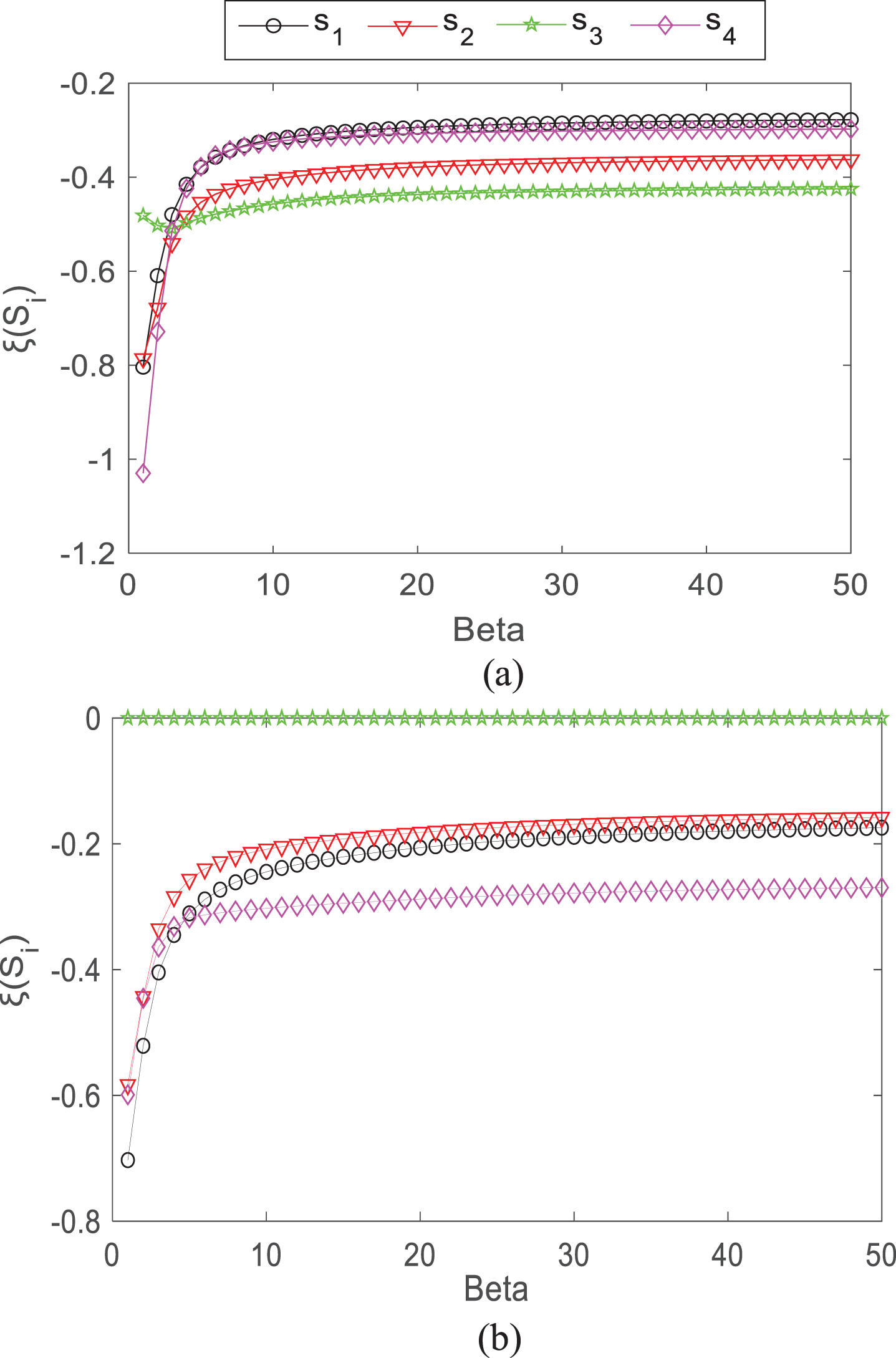
The results obtained from Figs. 1., 2. and 3 are shown in Table 3. In terms of simplicity: S1 = 1, S2 = 2, S3 = 3, S4 = 4.
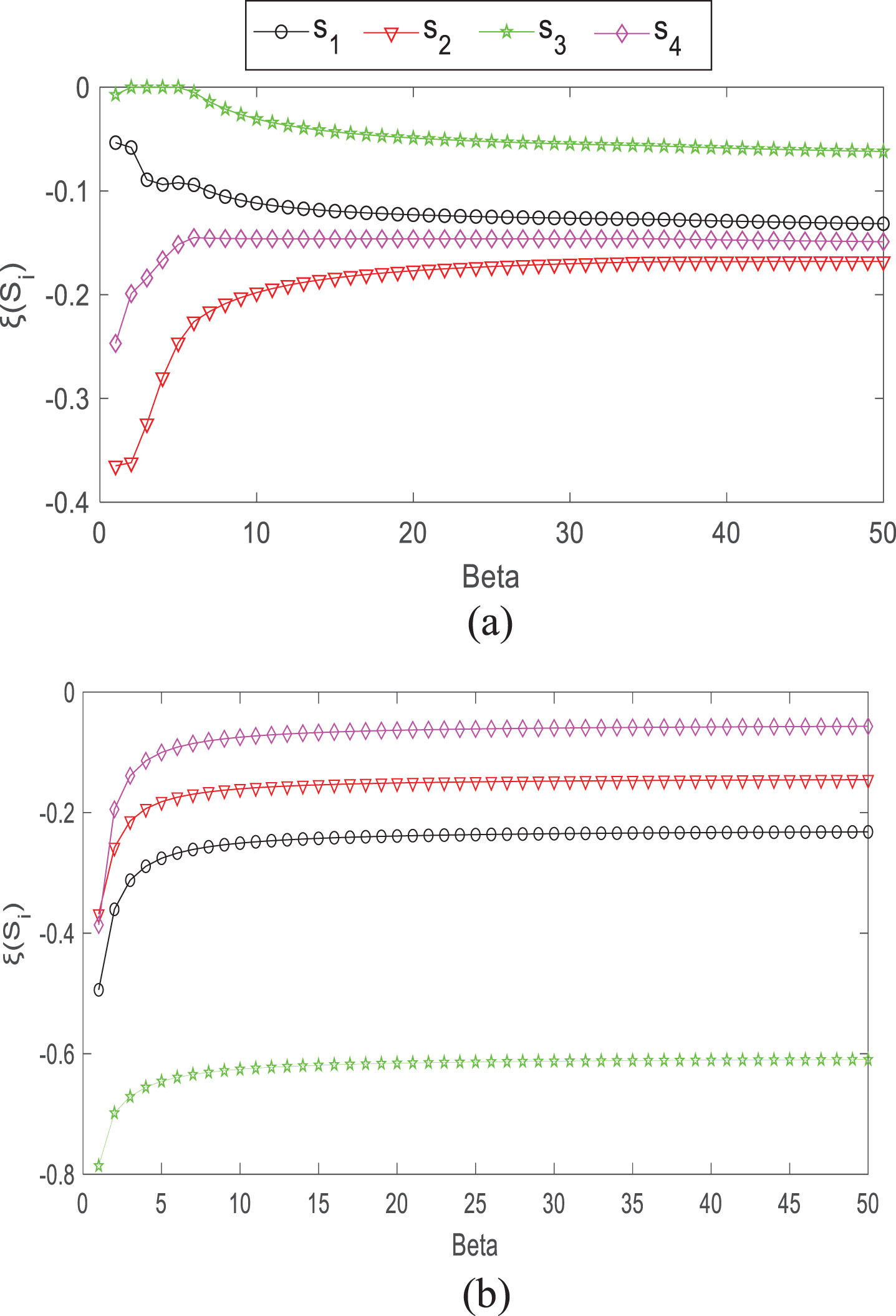
FFDWA (a) and FFDWG (b) aggregations results with different beta parameter.
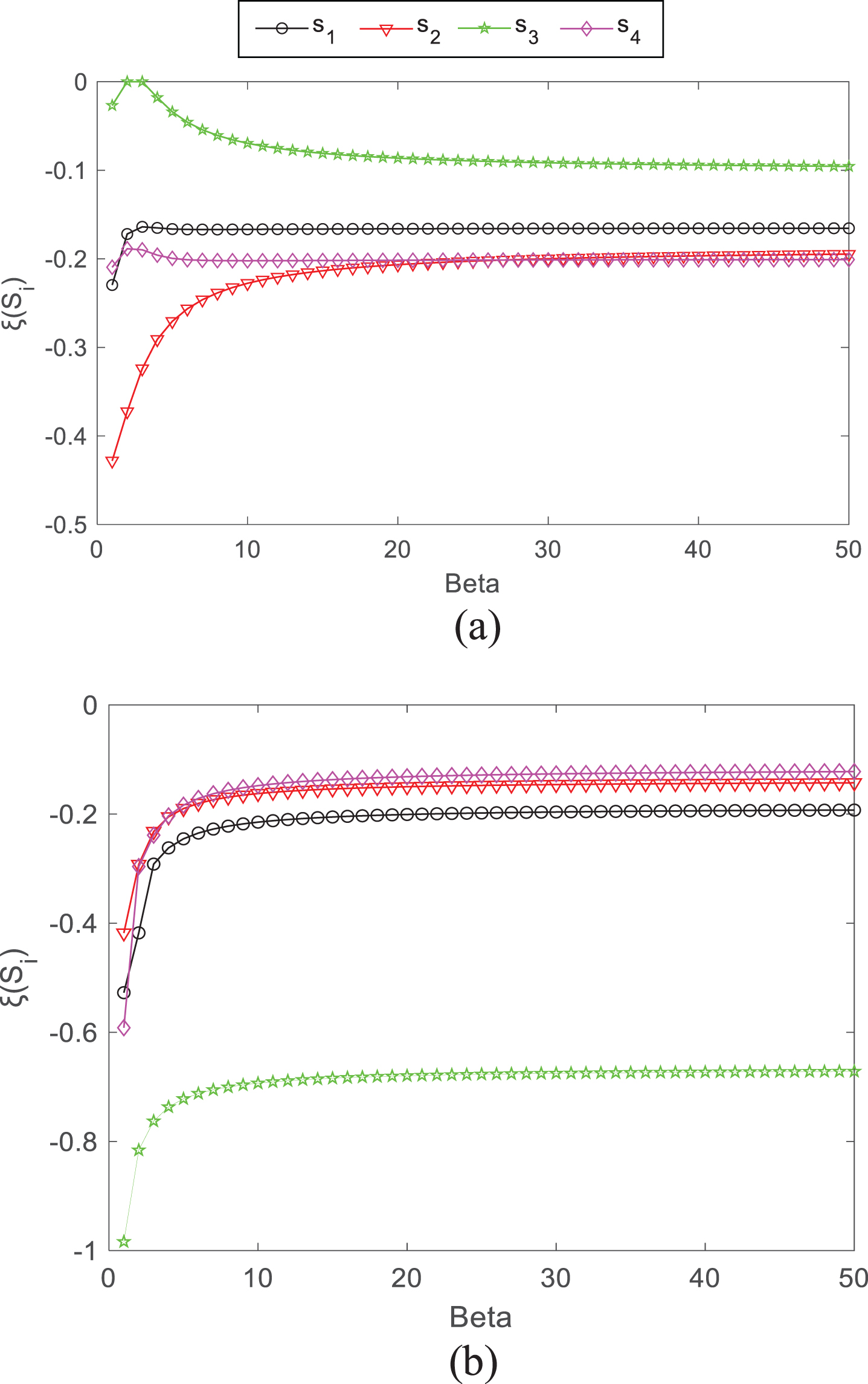
FFDOWA (a) and FFDOWG (b) aggregations results with different beta parameter.
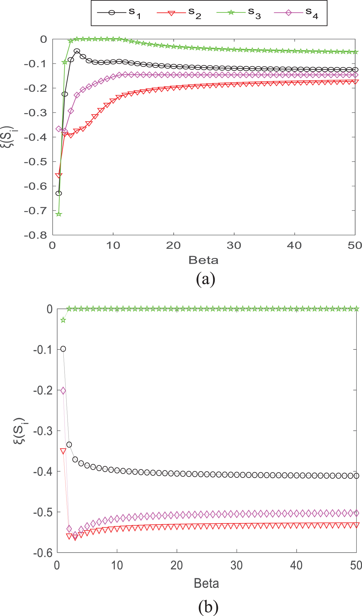
FFDHWA (a) and FFDHWG (b) aggregations results with different beta parameter.
Considering Table 3, we can observe the effect of the Dombi (beta) parameter for β = 50. After beta greater than 20, revised closeness values are observed to be stable. Because of the large variability in small values of beta, large values of beta are also taken into consideration. The optimal ranking order of the four places is S3 > S1 > S4 > S2 and the best alternative is S3. Considering all the existing aggregation functions on FFSs, the Dombi produces consistent and effective results.
Dombi and Existing Aggregation Methods
Table 4 shows a comparison of different methods. Among studies, it is seen that the Dombi operator gives consistent results on FFSs.
Comparison of different methods
The subject of the second problem consists of the selection of bridge construction. Bridge data information explored the construction of the concrete-based bridge superstructure for the Suhua Highway Alternative Road Project in Taiwan. Chen/Wang and Chen focus on this problem in many studies [5–7, 38]. On the other hand, with FFSs for selection of bridge construction solution searched [35]. There are four commonly used methods for bridge construction. Methods: the advanced shoring method (S1), the incremental launching method (S2), the balanced cantilever method (S3) and the precast segmental method (S4). Eight criteria were determined to evaluate the methods of bridge construction. Consisting of durability (C1), damage cost (C2), construction cost (C3), traffic effect (C4), site condition (C5), climatic condition (C6), landscape (C7) and environmental impact (C8). Durability and site conditions are benefit types, remaining criteria are cost type. Table 5 contains the data.
Fermatean fuzzy decision matrix
Fermatean fuzzy decision matrix
The matrix in Table 5 is taken from [35]. Furthermore, as in step 1, the normalized version is in Table 6. C1 and C5 benefit type, C2, C3, C4, C6, C7 and C8 cost type.
Normalized Fermatean fuzzy decision matrix
Let C = {C1, C2, C3, C4, C5, C6, C7, C8} be the set of criteria and let S ={ S1, S2, S3, S4 } be the set of alternatives. The weights of the criteria are given as w = (0.142875, 0.059524, 0.214251, 0.142875, 0.119048, 0.059524, 0.166665) T .
The Dombi parameter has different effects on arithmetic and geometric aggregations. FFSs, with order and hybrid of aggregation methods are expressed more accurately. Furthermore, in the FFDWA and FFDWG operators, weights are used according to the fuzzy values given. In the FFDOWA and FFDOWG operators, weights are used in the order of the Fermatean fuzzy values. But in both cases, they use their own weight. On the other hand, FFDHWA and FFDHWG reflect the order positions and degree of given Fermatean fuzzy values (Score -based).
FFSs, interval IFSs, interval PFSs are applied to the bridge construction selection problem [5–10, 38]. The results were also compared in this study. The applicability of Dombi aggregation methods in decision-making mechanisms is presented with comparisons. In the following figures, the revised closeness values for each Dombi aggregation according to the parameters are given
Although rare fluctuations appear in arithmetic operators, geometric operators appear to be stable. This situation depends on the Dombi parameter. While arithmetic operators depend on Dombi parameter, it can be said that geometric operators are more independent on parameter Dombi parameter.
Table 7 shows the results for β = 50. In all methods, a single ranking was included since the ranking resulting from the closeness average of β values and the ranking for β = 50 are the same but except for FFDWG. The closeness average value for FFDWG is given. Considering Fig. 4a, when β ∈ [1, 2], then ranking order S1 > S3 > S2 > S4. After β ⩾ 3, it is seen to be stable and S1 > S4 > S2 > S3 ranking is obtained. For FFDWA the best alternative is S1. In Fig. 4b, when β ∈ [1, 27], S3 > S2 > S4 > S1, for remaining β values S2 > S3 > S4 > S1. But considering all β values, the average result is ranking S3 > S2 > S4 > S1. So, for FFDWG total ranking order S3 > S2 > S4 > S1 obtained. So, for FFDWG the best alternative is S3. According to Fig. 5a, when β ∈ [1, 2], then ranking order S3 > S1 > S2 > S4. For β ∈ [5, 7], ranking order S4 > S1 > S2 > S3. But when β ∈ [3, 4] and β ∈ [8, 50] ranking order S1 > S4 > S2 > S3 obtained. So, For FFDOWA the best alternative is S1. According to Fig. 5b, For β ∈ [1, 4], ranking order S3 > S2 > S4 > S1. When β ∈ [5, 50] ranking order S3 > S2 > S1 > S4 obtained. Hence, for FFDOWG the best alternative is S3. Considering Fig. 6a, ordering varies at lower values of β. Therefore, the best alternative ranges are given. When β ∈ [1, 2], the best alternative is S3, for β ∈ [3, 50], the best alternative is S1. So, for FFDHWA total ranking order S1 > S4 > S2 > S3 and the best alternative is S1. Finally, Considering Fig. 6b, When β ∈ [1, 2], ranking is S3 > S1 > S2 > S4 and for β = 3 ranking is S1 > S4 > S2 > S3. When β ∈ [4, 50], the total ranking order is S1 > S3 > S4 > S2. Hence, for FFDHWG the best alternative S1 obtained. As a result, the best alternatives are S1 or S3. Considering all Dombi operators, the best alternative is S1. The proposed method is compared with other studies in Table 8. Ranking results are consistent with other existing methods. On the other hand, it can be said that arithmetic operators are more stable in itself. However, geometric operators depend much less on the Dombi parameter.
Dombi and existing aggregation methods
Dombi and existing aggregation methods
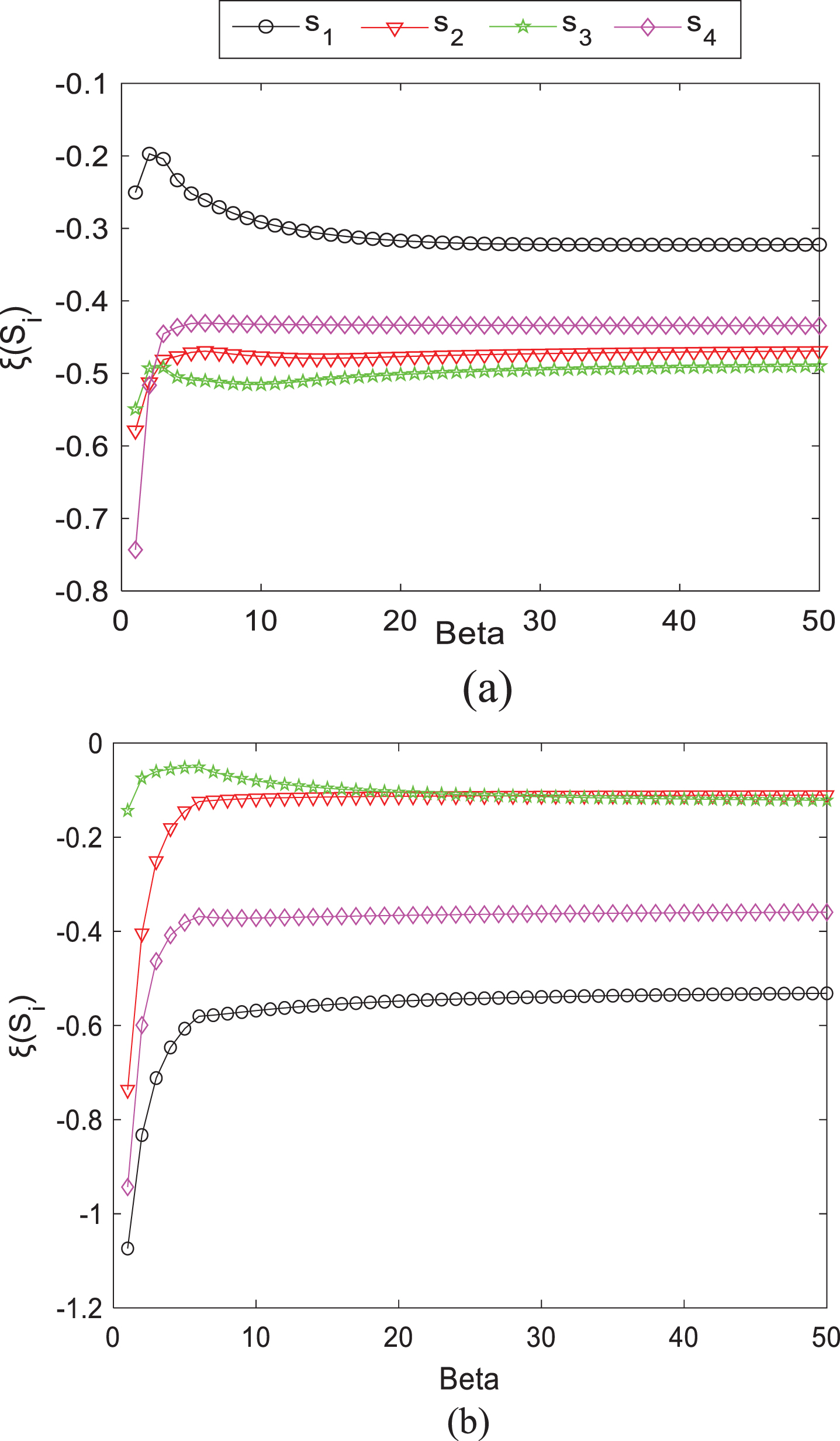
FFDWA (a) and FFDWG (b) aggregations results with different beta parameter.
FFDOWA (a) and FFDOWG (b) aggregations results with different beta parameter.
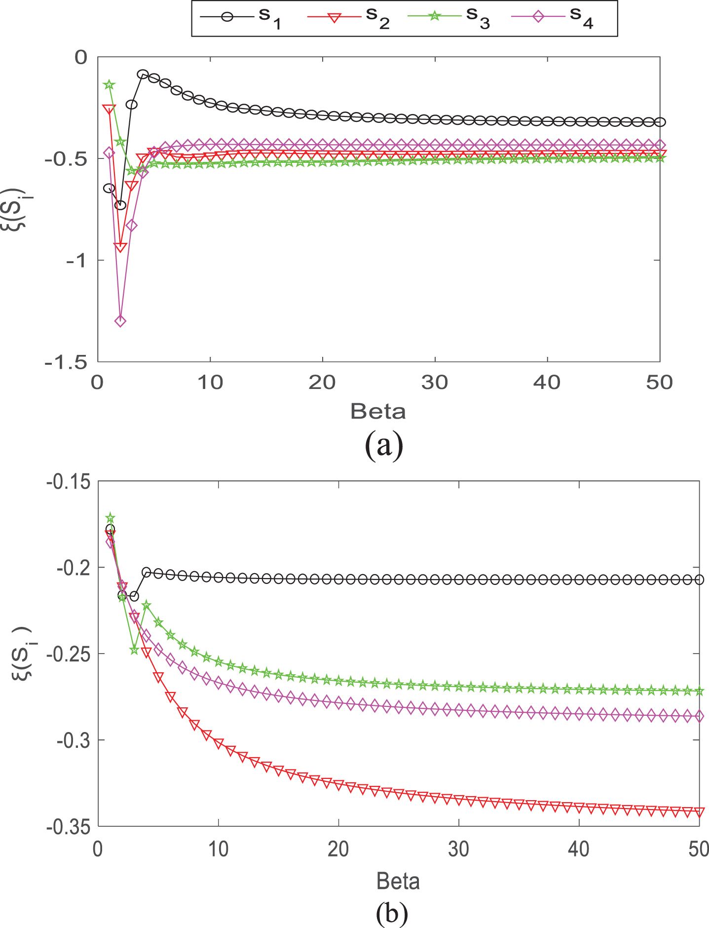
FFDHWA (a) and FFDHWG (b) aggregations results with different beta parameter.
Comparison of different methods
In this study, it is aimed to construct a more sensitive structure by using Dombi operators on FFSs. These operators are FFDWA, FFDWG, FFDOWA, FFDOWG, FFDHWA, FFDHWG operators. The changing beta parameter of Dombi operator provides flexibility. After beta greater than 20, beta values are observed to be stable. In addition, the idempotency, boundedness and monotonicity properties of Dombi operators on FFSs are mentioned. Finally, the TOPSIS method was extended with FFSs. Since FFSs are the extended version of intuitionistic fuzzy sets and Pythagorean fuzzy sets, FFSs can be said to give more flexible and more consistent results. In future studies, FFSs can be hybridized with different MCDM methods. Such as, Multimoora method [3], Vikor method [32]. On the other hand, FFSs with Dombi operator can be applied in several areas such as supplier selection, airline company and recommender system. Furthermore, the linguistic sets of FFSs sets are mentioned in the study [24]. As a next study, taking into account the criteria-based scores given to airline companies, linguistic variables with Dombi aggregation FFSs can be created and the best airline company can be selected according to the criteria.
Conflicts of interest
The authors declare that there is no conflict of interest regarding the publication of this paper.
Footnotes
Acknowledgments
This work is supported by scientific research project of Eskisehir Technical University under Grant 20DRP041.