Extensions of power aggregation operators for decision making based on complex picture fuzzy knowledge

Abstract

This article puts forward an innovative notion of complex picture fuzzy set (CPFS) which is particularly an extension and a generalization of picture fuzzy sets (PFSs) by the addition of phase term in the description of PFSs. The uniqueness of CPFS lies in the capability to manage the uncertainty and periodicity, simultaneously, due to the presence of phase term which broadens the range of CPFS from a real plane to the complex plane of unit disk. We describe and verify the fundamental operations and properties of CPFSs. We introduce the aggregation operators, namely; complex picture fuzzy power averaging and complex picture fuzzy power geometric operators in CPFSs environment, based on weighted and ordered weighted averaging and geometric operators. We construct multi-criteria decision making (MCDM) problem, using these operators and describe a numerical example to illustrate the validity and competence of this article. Finally, we discuss the advantages of this generalized concept of aggregation technique and analyze a comparative study to demonstrate the superiority and consistency of our model.

Keywords

Complex picture fuzzy set power aggregation operators multi-criteria decision making

1 Introduction

For selecting the optimal alternative(s) from the expedient set of accessible data, the multi-criteria decision making (MCDM) [17] is one of the most ubiquitous and an important authentic technique. Generally, a decision expert or a group of decision experts [33] is needed to evaluate a report about the alternatives by examining various given criteria. Many researchers had done a significant work to solve the MCDM issues under the fields of fuzzy set (FS) [53], intuitionistic fuzzy set (IFS) [9] and under some generalized fields [3, 4]. An influential and considerable study has been done by Li et al. [31, 32] in the field of generalized orthopair fuzzy sets to solve the decision making problems. Thus, for the certain acknowledgements the decision experts have to employ fuzzy variables. Many researchers have been made different efforts to solve the MCDM issues by utilizing various aggregation operators [12 , 38] and distance measure [19, 40] under different data sets. Aggregation operator (AO) is a mathematical function which converts the set of data or inputs into single datum. Aggregation operators play a significant role in decision-making processes. An ordered weighted averaging (OWA) and ordered weighted geometric (OWG) operators were introduced by Yager [51] and Chiclana et al. [14], respectively, in which they assigned the weights to all values of set or data with respect to their ranking order. Lin and Xu et al. [25] presented the OWA operators whose weights can be determined by using kernal density estimation. Yager [49] had utilized the AOs for the fuzzy systems modeling. With the intuitionistic fuzzy (IF) data, Xu [45] proposed the weighted averaging (WA) operator and Xu and Yager [47] introduced the geometric AOs. Lin et al. [22] introduced the heronian mean AOs in the generalized field of fuzzy sets. Liu and Wang [30] proposed the MCDM technique for the IFSs. To solve the MCDM issues Ye [52] proposed the hybrid geometric and averaging operators with IFS information. For the aggregation of various choices of experts to select the alternatives, the most appropriate aggregation operator must be chosen, among all of these distinct notions. An interrelated element among the alternatives is the most imperative element to be erected during an aggregation plan. But it is concluded from all the discussed strategies that the choices of expert(s) are independent and there is an absence of basic interrelationship among the expert opinions. To deal with such circumstances, Yager [50] introduced the power aggregation (PA) operators, which exhibits the relation among the choices and these choices strengthen up each other during the aggregation plan. Later on, Wei et al. [44] proposed the PA operators under fuzzy environment and Xu and Yager [48] presented the PA operators for the IFSs. Xu [46] had solved the MCDM issues by using PA operator for the IFSs. However, the environment of FSs and IFSs give the incomplete information about the elements of data set. Cuong [16] presented the innovative idea of picture fuzzy set (PFS) which is characterized by the non-membership, membership and neutral membership functions which shows the information about the human decisions like; yes, refrain, no and refusal. He [15] also gave some results on PFS. Khan et al. [21] introduced the Einstein operations on PFSs. Recently, Wei [43] utilized the Hamachar operators in PFSs. Garg [18] also contributed to present the aggregation strategy under PFSs environment. Lin et al. [23] introduced a novel concept, namely; MULTIMOORA of solving MCDM technique by utilizing PFS information. The aggregation operators utilized by some authors under different environments which have not been discussed over here are given in [29, 42].

It has been figured out that the MCDM issues solved as for above existing studies in FS, IFS and extended sets such as PFSs, environments are only capable to handle the vagueness and ambiguity of the data. The ignorance in time period and insensitivity of data can not be dealt by all these models. Though the periodicity and the uncertainty of the data can be handled simultaneously by a complex data set. Ramot et al. [34, 35] had put forward the concept of complex fuzzy set (CFS) to handle these situations. They proposed that the membership degree of a CFS is given as μe^{iφ
_μ} whose range is extended to the unit disk in a complex plane, where μ ∈ [0, 1] and φ_μ ∈ [0, 2π] . Some operational laws and properties of a CFS were proposed by Zhang et al. [54]. A wide range of applications of CFSs have been introduced since its appearance in various real life fields, e.g., audio databases, biometric process, medical researches and etc. Bi et al. [10, 11] introduced the geometric and arithmetic AOs in the field of CFSs. Akram and Bashir [1] proposed the innovative notion of ordered weighted quadratic averaging operators using CF data. The CFS is not sufficient to tell the discrepancies of an element in the data set. Then the generalization of CFS, complex intuitionistic fuzzy set (CIFS) was recommended by Alkouri and Salleh [8] in which they had introduced the membership as well the non-membership of an element. They defined union, complement and the intersection of the CIFS. Later on, Rani and Garg [36] proposed the power AOs, using CIFS data to solve the MCDM problems. But CIFS is not capable to deal with slightly ignored data such as CIFS only exhibits values of membership degrees of an element of a data set in a complex plane but it can not tell about the abstain choice (neutral value) or refusal of an information. This lack of information in CIFS theory leads us to a novel concept of complex picture fuzzy set (CPFS) which is characterized by membership, neutral membership and non-membership values in a unit disk of a complex plane. For some remaining discussion about aggregation operators and MCDM techniques which is not discussed here, the readers are referred to [2 , 41].

The CPFS is more general than the PFS, CFS and CIFS due to the wider range because of the presences of neutral membership along with existing membership degrees. CPFSs can inform about an object with much more details and can discuss uncertainties and periodicity concurrently more generally than the other existing models. The motivation of proposed model is summarized as follows:

The membership degrees of a CPFS are complex valued consisting of amplitude and phase terms. The amplitude term of neutral membership (membership, non-membership) function refers to the abstain (acceptance, nonacceptance) value whereas the phase term corresponding to neutral membership (membership, non-membership) function shows the further material, generally about periodicity.

The CPFS is differentiated from the established model of PFS by the new specification of phase term. Because the PFS can only handle one dimensional data whose outcome is a loss in data. However, in real life phenomena, we deal with the situations in which the second dimension is necessary to be added in all membership degrees.

The power AOs utilized in the proposed model are more appropriate than any other aggregation plan to solve the the MCDM problems as these operators have ability to exhibit the interdependence of arguments and most importantly the preferences strengthen up each other during the aggregation process.

The presented approach is based on complex picture fuzzy (CPF) data whose expedient potential to represent the two dimensional phenomena makes it preferable to handle the spontaneous and uncertain data. Secondly, the PA operators become more advantageous and effective under the generalized environment of CPFS to resolve the real life complex issues and constructive problem.

The main contributions of this paper are:

The notion of CPFS is interpreted with some fundamental operations and properties which are discussed and verified. Score and accuracy functions are also defined for the CPFSs.

The PA technique including averaging and geometric operators, is examined under CPFS environment. Some results and properties of PA operators are also described by utilizing CPF information.

The advantages and significance of the PA operators under the generalized environment of CPFS are interpreted by analyzing the MCDM scheme. Finally, a comparative study is explained to exhibit the superiority and authenticity of the proposed aggregation operators.

The layout of this manuscript is interpreted as follows: We describe some fundamental notions in Section 2 which are helpful to understand this manuscript. Section 3 presents the novel concept of complex picture fuzzy set (CPFS). Here, we explain some properties and operational laws for CPFS. We also define the score and accuracy functions of the CPFSs. Section 4 exhibits analyzed results and properties of power averaging AOs including weighted and ordered weighted averaging operators under CPFSs environment. In Section 5, we put forward the concept of CPFPG, CPFPWG and CPFPOWG operators. We prove some properties and results for these operators. In Section 6, we discuss a MCDM model to evaluate the best alternative with a case study and the validity criteria to prove the consistency of proposed work. In Section 7, we compare the presented model with some already existing techniques to exhibit the superiority and influence of our manuscript and discuss some merits of proposed model. Finally, we write the concluding remarks and some future directions, in Section 8.

2 Preliminaries

Definition 2.1. [35] A set $ℂ,$ defined on a universe $J$ given as follows: $\begin{matrix} ℂ & = & {(j, υ_{ℂ} (j)) | j \in J}, \end{matrix}$ is called complex fuzzy set (CFS) such that the membership function $υ_{ℂ} (j)$ refers a complex-valued grade of membership to any element $j \in J .$ Thus $υ_{ℂ} (j)$ may receive all the values from a unit disk in a complex plane, i.e., $υ_{ℂ} (j) = a_{ℂ} (j) e^{i α_{ℂ} (j)},$ where $i = \sqrt{- 1},$ $a_{ℂ} (j)$ and $α_{ℂ} (j)$ both are real and $a_{ℂ} (j) \in [0, 1],$ $α_{ℂ} (j) \in [0, 2 π] .$ $a_{ℂ} (j)$ and $α_{ℂ} (j)$ are called the amplitude and phase terms, respectively.

Definition 2.2. [8] A set $I,$ defined on a universe $J$ expressed as follows: $\begin{matrix} I & = & {(j, υ_{I} (j), ς_{I} (j)) | j \in J} \end{matrix}$ is called complex intuitionistic fuzzy set (CIFS) such that $| υ_{I} (j) + ς_{I} (j) | \leq 1,$ where $υ_{I} (j)$ and $ς_{I} (j))$ are the membership and non-membership functions, respectively, that assign a complex-valued membership degrees to any element $j \in J .$ Thus $υ_{I} (j)$ and $ς_{I} (j))$ and their sum may receive all the values from a unit disk in a complex plane, i.e., $υ_{I} (j) = a_{I} (j) e^{i α_{υ_{I}} (j)}$ and $ς_{I} (j) = a_{I}^{'} (j) e^{i α_{ς_{I}} (j)},$ where $i = \sqrt{- 1},$ $a_{I} (j)$ and $a_{I}^{'} (j)$ both are real and belong to the interval [0, 1] with the restriction $0 \leq a_{I} (j) + a_{I}^{'} (j) \leq 1 .$ Also, $α_{υ_{I}} (j), α_{ς_{I}} (j) \in [0, 2 π]$ are real valued with the restriction $0 \leq α_{υ_{I}} (j) + α_{ς_{I}} (j) \leq 2 π .$

Definition 2.3. [36] The score and the accuracy functions of a CIFN $I = ((υ, α_{υ}), (ς, α_{ς}))$ are given as follows: $\begin{matrix} S (I) & = & υ - ς + \frac{1}{2 π} (α_{υ} - α_{ς}) \\ ℍ (I) & = & υ + ς + \frac{1}{2 π} (α_{υ} + α_{ς}), \end{matrix}$ respectively. Thus, if $I$ and $L$ are two CIFNs, then $L ≺ I,$ if

$S (L) 〈 S (I),$ or

$S (I) = S (L) \land ℍ (I) 〉 ℍ (L)$

Definition 2.4. [37] The distance measures between any two CIFNs $I = ((υ_{I}, α_{υ_{I}}), (ς_{I}, α_{ς_{I}}))$ and $L = ((υ_{L}, α_{υ_{L}}), (ς_{L}, α_{ς_{L}}))$ can be expressed as follows: $\begin{matrix} d (I, L) & = & \frac{1}{4} [| υ_{I} - υ_{L} | + | ς_{I} - ς_{L} | \\ + \frac{1}{2 π} (| α_{υ_{I}} - α_{υ_{L}} | + | α_{ς_{I}} - α_{ς_{L}} |)] . \end{matrix}$

Definition 2.5. [16] A set $W,$ defined on a universe $J$ denoted as follows: $\begin{matrix} W & = & {(j, μ_{W} (j), ζ_{W} (j), ν_{W} (j)) | j \in J} \end{matrix}$ is called picture fuzzy set (PFS) such that $μ_{W} (j),$ $ζ_{W} (j),$ $ν_{W} (j)$ ∈[0, 1] are called positive membership, neutral membership and negative membership functions, respectively, of the element j in $W$ with the condition $μ_{W} (j) + ζ_{W} (j) + ν_{W} (j) \leq 1 .$ The refusal membership function of a PFS is given as $1 - (μ_{W} (j) + ζ_{W} (j) + ν_{W} (j)),$ for all $j \in J .$

Definition 2.6. [50] The power averaging operator for a data set o_m = (m = 1, 2, …, p) can be determined as follows: $\begin{matrix} PA (o_{1}, o_{2}, \dots, o_{p}) & = & \frac{\sum_{m = 1}^{p} (1 + T (o_{m})) o_{m}}{\sum_{m = 1}^{p} (1 + T (o_{m}))}, \end{matrix}$ where $T (o_{m}) = \sum_{r = 1, r \neq m}^{p} Sup (o_{m}, o_{r}) .$ The similarity index Sup (o_m, o_r) is the support of o_m from o_r which obeys the following axioms:

Sup (o_m, o_r) ∈ [0, 1] .

Sup (o_m, o_r) = Sup (o_r, o_m) .

If |o_m - o_r| ≤ |o_k - o_l|, then Sup (o_m, o_r) ≥ Sup (o_r, o_m) .

3 Complex picture fuzzy sets

Definition 3.1. A complex picture fuzzy set (CPFS) ξ on a universe ϝ is expressed in the form: $\begin{matrix} ξ & = & 〈 (f, μ_{ξ} (f) e^{i α_{ξ} (f)}, ζ_{ξ} (f) e^{i γ_{ξ} (f)}, \\ ν_{ξ} (f) e^{i β_{ξ} (f)}) | f \in ϝ 〉, \end{matrix}$ where $i = \sqrt{- 1},$ μ_ξ (f) , ζ_ξ (f) , ν_ξ (f) ∈ [0, 1] are amplitude terms and α_ξ (f) , γ_ξ (f) , β_ξ (f) ∈ [0, 2π] are the phase terms of membership, neutral membership and non-membership degrees, respectively, which are restricted by the conditions μ_ξ (f) + ζ_ξ (f) + ν_ξ (f) ≤1 and α_ξ (f) + γ_ξ (f) + β_ξ (f) ≤2π, for all f ∈ ϝ . The degree of rejection of f in ξ is given as follows: $\begin{matrix} ℏ_{ξ} (f) & = & (1 - μ_{ξ} (f) - ζ_{ξ} (f) - ν_{ξ} (f)) \\ e^{i (2 π - α_{ξ} (f) - γ_{ξ} (f) - β_{ξ} (f))}, \end{matrix}$ for all f ∈ ϝ .

Definition 3.2. For any two CPFSs on a universe ϝ, the operations of inclusion, intersection, union and compliment are interpreted in the following:

ξ₁ ⊆ ξ₂ if and only if μ_ξ
₁ (f) ≤ μ_ξ
₂ (f) , ζ_ξ
₁ (f) ≥ ζ_ξ
₂ (f) and ν_ξ
₁ (f) ≥ ν_ξ
₂ (f) , for amplitude terms and α_ξ
₁ (f) ≤ α_ξ
₂ (f) , γ_ξ
₁ (f) ≥ γ_ξ
₂ (f) and β_ξ
₁ (f) ≥ β_ξ
₂ (f) , for phase terms, for all f ∈ ϝ .

ξ₁ ∩ ξ₂ = < (f, min(μ_ξ
₁ (f) , μ_ξ
₂ (f)) e^{imin(α_{ξ
₁}(f),α_{ξ
₂}(f))}, max(ζ_ξ
₁ (f) , ζ_ξ
₂ (f)) e^{imax(γ_{ξ
₁}(f),γ_{ξ
₂}(f))}, max(ν_ξ
₁ (f) , ν_ξ
₂ (f)) e^{imax(β_{ξ
₁}(f),β_ξ₂(f))}) |f ∈ ϝ > .

ξ₁ ∪ ξ₂ = < (f, max(μ_ξ
₁ (f) , μ_ξ
₂ (f)) e^{imax(α_{ξ
₁}(f),α_{ξ
₂}(f))}, min(ζ_ξ
₁ (f) , ζ_ξ
₂ (f)) e^{imin(γ_{ξ
₁}(f),γ_{ξ
₂}(f))}, min(ν_ξ
₁ (f) , ν_ξ
₂ (f)) e^{imin(β_{ξ
₁}(f),β_ξ₂(f))}) |f ∈ ϝ > .

$\bar{ξ} = 〈 (f, ν_{ξ} (f) e^{i β_{ξ} (f)}, ζ_{ξ} (f) e^{i γ_{ξ} (f)}, μ_{ξ} (f) e^{i α_{ξ} (f)}) | f \in ϝ 〉 .$

For convenience, we suppose that ξ = (μ_ξe^{iα
_ξ}, ζ_ξe^{iγ
_ξ}, ν_ξe^{iβ
_ξ}) is a complex picture fuzzy number (CPFN), where μ_ξ (f) , ζ_ξ (f) , ν_ξ (f) ∈ [0, 1] and α_ξ (f) , γ_ξ (f) , β_ξ (f) ∈ [0, 2π] restricted with conditions μ_ξ (f) + ζ_ξ (f) + ν_ξ (f) ≤1 and α_ξ (f) + γ_ξ (f) + β_ξ (f) ≤2π, for all f ∈ ϝ , respectively.

Definition 3.3. The score function S of a CPFN ξ = (μ_ξe^{iα
_ξ}, ζ_ξe^{iγ
_ξ}, ν_ξe^{iβ
_ξ}) is presented as follows: $\begin{matrix} S (ξ) & = & (μ - ζ - ν) + \frac{1}{2 π} (α - γ - β), \end{matrix}$ where S (ξ) ∈ [-2, 2] . The score function is essential for the ranking of CPFNs.

Example 3.1. Let ξ₁ = (0.2e^i0.1π, 0.3e^i0.8π, 0.4e^i0.3π) and ξ₂ = (0.4e^i0.6π, 0.1e^i1.1π, 0.2e^i0.2π) be two CPFNs. Then S (ξ₁) = -1 and S (ξ₂) = -0.25 . This shows that S (ξ₂) > S (ξ₁) and so, ξ₂ > ξ₁ .

Sometimes score function fails to rank the CPFNs. In case, if ξ₁ = (0.3e^i0.1π, 0.3e^i0.8π, 0.4e^i0.3π) and ξ₂ = (0.2e^i0.6π, 0.3e^i1.1π, 0.2e^i0.2π) , then S (ξ₁) = S (ξ₂) , which makes it impossible to know the bigger value. The accuracy function, given as follows, can handle this situation.

Definition 3.4. The accuracy function H of a CPFN ξ = (μ_ξe^{iα
_ξ}, ζ_ξe^{iγ
_ξ}, ν_ξe^{iβ
_ξ}) is presented as follows: $\begin{matrix} H (ξ) & = & (μ + ζ + ν) + \frac{1}{2 π} (α + γ + β), \end{matrix}$ where H (ξ) ∈ [0, 2] .

According to the accuracy (H) and score (S) functions, the order relation between any two CPFNs is defined in the following:

Definition 3.5. Let ξ₁ = (μ_{ξ
₁}e^{iα
_{ξ
₁}}, ζ_{ξ
₁}e^{iγ
_{ξ
₁}}, ν_{ξ
₁}e^{iβ
_{ξ
₁}}) and ξ₂ = (μ_{ξ
₂}e^{iα
_{ξ
₂}}, ζ_{ξ
₂}e^{iγ
_{ξ
₂}}, ν_{ξ
₂}e^{iβ
_{ξ
₂}}) be two CPFNs, then their score functions and accuracy functions are given as follows: $\begin{matrix} S (ξ_{1}) & = & (μ_{ξ_{1}} - ζ_{ξ_{1}} - ν_{ξ_{1}}) + \frac{1}{2 π} (α_{ξ_{1}} - γ_{ξ_{1}} - β_{ξ_{1}}), \\ S (ξ_{2}) & = & (μ_{ξ_{2}} - ζ_{ξ_{2}} - ν_{ξ_{2}}) + \frac{1}{2 π} (α_{ξ_{2}} - γ_{ξ_{2}} - β_{ξ_{2}}), \\ H (ξ_{1}) & = & (μ_{ξ_{1}} + ζ_{ξ_{1}} + ν_{ξ_{1}}) + \frac{1}{2 π} (α_{ξ_{1}} + γ_{ξ_{1}} + β_{ξ_{1}}), \\ H (ξ_{2}) & = & (μ_{ξ_{2}} + ζ_{ξ_{2}} + ν_{ξ_{2}}) + \frac{1}{2 π} (α_{ξ_{2}} + γ_{ξ_{2}} + β_{ξ_{2}}) . \end{matrix}$ For two CPFSs ξ₁ < ξ₂, if S (ξ₁) < S (ξ₂). There are two conditions if S (ξ₁) = S (ξ₂) , given as follows:

If H (ξ₁) < H (ξ₂) , then ξ₁ < ξ₂ .

If H (ξ₁) = H (ξ₂) , then ξ₁ = ξ₂, i.e., ξ₁ and ξ₂ exhibit the same information.

Definition 3.6. Let ξ₁ = (μ_{ξ
₁}e^{iα
_{ξ
₁}}, ζ_{ξ
₁}e^{iγ
_{ξ
₁}}, ν_{ξ
₁}e^{iβ
_{ξ
₁}}) and ξ₂ = (μ_{ξ
₂}e^{iα
_{ξ
₂}}, ζ_{ξ
₂}e^{iγ
_{ξ
₂}}, ν_{ξ
₂}e^{iβ
_{ξ
₂}}) be two CPFNs, then

$\bar{ξ_{1}} = 〈 (f, ν_{ξ_{1}} (f) e^{i β_{ξ_{1}} (f)}, ζ_{ξ_{1}} (f) e^{i γ_{ξ_{1}} (f)}, μ_{ξ_{1}} (f) e^{i α_{ξ_{1}} (f)}) | f \in ϝ 〉 .$

ξ₁ ∧ ξ₂ = < (f, min(μ_ξ
₁ (f) , μ_ξ
₂ (f)) e^{imin(α_{ξ
₁}(f),α_{ξ
₂}(f))}, max(ζ_ξ
₁ (f) , ζ_ξ
₂ (f)) e^{imax(γ_{ξ
₁}(f),γ_{ξ
₂}(f))}, max(ν_ξ
₁ (f) , ν_ξ
₂ (f)) e^{imax(β_{ξ
₁}(f),β_ξ₂(f))}) |f ∈ ϝ > .

ξ₁ ∨ ξ₂ = < (f, max(μ_ξ
₁ (f) , μ_ξ
₂ (f)) e^{imax(α_{ξ
₁}(f),α_{ξ
₂}(f))}, min(ζ_ξ
₁ (f) , ζ_ξ
₂ (f)) e^{imin(γ_{ξ
₁}(f),γ_{ξ
₂}(f))}, min(ν_ξ
₁ (f) , ν_ξ
₂ (f)) e^{imin(β_{ξ
₁}(f),β_ξ₂(f))}) |f ∈ ϝ > .

$ξ_{1} \oplus ξ_{2} = 〈 (μ_{ξ_{1}} + μ_{ξ_{2}} - μ_{ξ_{1}} μ_{ξ_{2}}) e^{i 2 π (\frac{α_{ξ_{1}}}{2 π} + \frac{α_{ξ_{2}}}{2 π} - \frac{α_{ξ_{1}}}{2 π} \frac{α_{ξ_{2}}}{2 π})}, ζ_{ξ_{1}} e^{i γ_{ξ_{1}}} \cdot ζ_{ξ_{2}} e^{i γ_{ξ_{2}}}, ν_{ξ_{1}} e^{i β_{ξ_{1}}} \cdot ν_{ξ_{2}} e^{i β_{ξ_{2}}} 〉 .$

$ξ_{1} \otimes ξ_{2} = 〈 μ_{ξ_{1}} e^{i α_{ξ_{1}}} \cdot μ_{ξ_{2}} e^{i α_{ξ_{2}}}, (ζ_{ξ_{1}} + ζ_{ξ_{2}} - ζ_{ξ_{1}} ζ_{ξ_{2}}) e^{i 2 π (\frac{γ_{ξ_{1}}}{2 π} + \frac{γ_{ξ_{2}}}{2 π} - \frac{γ_{ξ_{1}}}{2 π} \frac{γ_{ξ_{2}}}{2 π})}, (ν_{ξ_{1}} + ν_{ξ_{2}} - ν_{ξ_{1}} ν_{ξ_{2}}) e^{i 2 π (\frac{β_{ξ_{1}}}{2 π} + \frac{β_{ξ_{2}}}{2 π} - \frac{β_{ξ_{1}}}{2 π} \frac{β_{ξ_{2}}}{2 π})} 〉,$ where $μ_{ξ_{1}} e^{i α_{ξ_{1}}} \cdot μ_{ξ_{2}} e^{i α_{ξ_{2}}} = μ_{ξ_{1}} \cdot μ_{ξ_{2}} e^{i 2 π (\frac{α_{ξ_{1}}}{2 π} \cdot \frac{α_{ξ_{2}}}{2 π})} .$ Similar expression holds for ζ_ξ
₁e^{iγ
_{ξ
₁}} · ζ_ξ
₂e^{iγ
_{ξ
₂}} and ν_ξ
₁e^{iβ
_{ξ
₁}} · ν_ξ
₂e^{iβ
_{ξ
₂}} .

$ℵ ξ_{1} = 〈 (1 - (1 - μ_{ξ_{1}})^{ℵ}) e^{i 2 π (1 - (1 - \frac{α_{ξ_{1}}}{2 π})^{ℵ})}, ζ_{ξ_{1}}^{ℵ} e^{i 2 π (\frac{γ_{ξ_{1}}}{2 π})^{ℵ}}, ν_{ξ_{1}}^{ℵ} e^{i 2 π (\frac{β}{2 π})^{ℵ}} 〉, ℵ 〉 0 .$

$ξ_{1}^{ℵ} = 〈 μ_{ξ_{1}}^{ℵ} e^{i 2 π (\frac{α}{2 π})^{ℵ}}, (1 - (1 - ζ_{ξ_{1}})^{ℵ}) e^{i 2 π (1 - (1 - \frac{γ_{ξ_{1}}}{2 π})^{ℵ})}, (1 - (1 - ν_{ξ_{1}})^{ℵ}) e^{i 2 π (1 - (1 - \frac{β_{ξ_{1}}}{2 π})^{ℵ})} 〉, ℵ 〉 0 .$

Theorem 3.1. Let ξ₁ = (μ_{ξ
₁}e^{iα
_{ξ
₁}}, ζ_{ξ
₁}e^{iγ
_{ξ
₁}}, ν_{ξ
₁}e^{iβ
_{ξ
₁}}) and ξ₂ = (μ_{ξ
₂}e^{iα
_{ξ
₂}}, ζ_{ξ
₂}e^{iγ
_{ξ
₂}}, ν_{ξ
₂}e^{iβ
_{ξ
₂}}) be two CPFNs, 0 ≤ ℵ , ℵ ₁, ℵ ₂ ≤ 1, then

ξ₁ ⊕ ξ₂ = ξ₂ ⊕ ξ₁ .

$(ξ_{1}^{ℵ_{1}})^{ℵ_{2}} = ξ_{1}^{ℵ_{1} ℵ_{2}} .$

ℵ (ξ₁ ⊕ ξ₂) = ℵ ξ₁ ⊕ ℵ ξ₂ .

ℵ₁ξ₁ ⊕ ℵ ₂ξ₁ = (ℵ ₁ + ℵ ₂) ξ₁ .

$(ξ_{1} \otimes ξ_{2})^{ℵ} = ξ_{1}^{ℵ} \otimes ξ_{2}^{ℵ} .$

$ξ_{1}^{ℵ_{1}} \otimes ξ_{1}^{ℵ_{2}} = ξ_{1}^{ℵ_{1} + ℵ_{2}} .$

Proof.

$\begin{matrix} ξ_{1} \oplus ξ_{2} & = & 〈 (μ_{ξ_{1}} + μ_{ξ_{2}} - μ_{ξ_{1}} μ_{ξ_{2}}) e^{i 2 π (\frac{α_{ξ_{1}}}{2 π} + \frac{α_{ξ_{2}}}{2 π} - (\frac{α_{ξ_{1}}}{2 π}) (\frac{α_{ξ_{2}}}{2 π}))}, ζ_{ξ_{1}} e^{i γ_{ξ_{1}}} ζ_{ξ_{2}} e^{i γ_{ξ_{2}}}, ν_{ξ_{1}} e^{i β_{ξ_{1}}} ν_{ξ_{2}} e^{i β_{ξ_{2}}} 〉 \\ = & 〈 (μ_{ξ_{2}} + μ_{ξ_{1}} - μ_{ξ_{2}} μ_{ξ_{1}}) e^{i 2 π (\frac{α_{ξ_{2}}}{2 π} + \frac{α_{ξ_{1}}}{2 π} - (\frac{α_{ξ_{2}}}{2 π}) (\frac{α_{ξ_{1}}}{2 π}))}, ζ_{ξ_{2}} e^{i γ_{ξ_{2}}} ζ_{ξ_{1}} e^{i γ_{ξ_{1}}}, ν_{ξ_{2}} e^{i β_{ξ_{2}}} ν_{ξ_{1}} e^{i β_{ξ_{1}}} 〉 \\ = & ξ_{2} \oplus ξ_{1} . \end{matrix}$

Since, ξ₁, ξ₂ are CPFNs $\begin{matrix} ℵ (ξ_{1} \oplus ξ_{2}) = & ℵ 〈 (μ_{ξ_{1}} + μ_{ξ_{2}} - μ_{ξ_{1}} μ_{ξ_{2}}) e^{i 2 π (\frac{α_{ξ_{1}}}{2 π} + \frac{α_{ξ_{2}}}{2 π} - (\frac{α_{ξ_{1}}}{2 π}) (\frac{α_{ξ_{2}}}{2 π}))}, ζ_{ξ_{1}} e^{i γ_{ξ_{1}}} ζ_{ξ_{2}} e^{i γ_{ξ_{2}}}, ν_{ξ_{1}} e^{i β_{ξ_{1}}} ν_{ξ_{2}} e^{i β_{ξ_{2}}} 〉 \\ = & 〈 (1 - (1 - (μ_{ξ_{1}} + μ_{ξ_{2}} - μ_{ξ_{1}} μ_{ξ_{2}}))^{ℵ}) e^{i 2 π (1 - (1 - ((\frac{α_{ξ_{1}}}{2 π}) + (\frac{α_{ξ_{2}}}{2 π}) - (\frac{α_{ξ_{1}}}{2 π}) (\frac{α_{ξ_{2}}}{2 π})))^{ℵ})}, \\ (ζ_{ξ_{1}} e^{i γ_{ξ_{1}}} ζ_{ξ_{2}} e^{i γ_{ξ_{2}}})^{ℵ}, (ν_{ξ_{1}} e^{i β_{ξ_{1}}} ν_{ξ_{2}} e^{i β_{ξ_{2}}})^{ℵ} 〉 \\ = & 〈 (1 - (1 - (μ_{ξ_{1}} + μ_{ξ_{2}} - μ_{ξ_{1}} μ_{ξ_{2}}))^{ℵ}) e^{i 2 π (1 - (1 - ((\frac{α_{ξ_{1}}}{2 π}) + (\frac{α_{ξ_{2}}}{2 π}) - (\frac{α_{ξ_{1}}}{2 π}) (\frac{α_{ξ_{2}}}{2 π})))^{ℵ})}, \\ (ζ_{ξ_{1}} e^{i γ_{ξ_{1}}} ζ_{ξ_{2}} e^{i γ_{ξ_{2}}})^{ℵ}, (ν_{ξ_{1}} e^{i β_{ξ_{1}}} ν_{ξ_{2}} e^{i β_{ξ_{2}}})^{ℵ} 〉 . \end{matrix}$ According to Definition 3.6, $\begin{matrix} ℵ ξ_{1} = & 〈 (1 - (1 - μ_{ξ_{1}})^{ℵ}) e^{i 2 π (1 - (1 - (\frac{α_{ξ_{1}}}{2 π}))^{ℵ})}, (ζ_{ξ_{1}} e^{i γ_{ξ_{1}}})^{ℵ}, (ν_{ξ_{1}} e^{i β_{ξ_{1}}})^{ℵ} 〉 . \\ ℵ ξ_{2} = & 〈 (1 - (1 - μ_{ξ_{2}})^{ℵ}) e^{i 2 π (1 - (1 - (\frac{α_{ξ_{2}}}{2 π}))^{ℵ})}, (ζ_{ξ_{2}} e^{i γ_{ξ_{2}}})^{ℵ}, (ν_{ξ_{2}} e^{i β_{ξ_{2}}})^{ℵ} 〉 . \\ ℵ ξ_{1} \oplus ℵ ξ_{2} = & 〈 ((1 - (1 - μ_{ξ_{1}})^{ℵ}) + (1 - (1 - μ_{ξ_{2}})^{ℵ}) - (1 - (1 - μ_{ξ_{1}})^{ℵ}) (1 - (1 - μ_{ξ_{2}})^{ℵ})) \\ e^{i 2 π ((1 - (1 - (\frac{α_{ξ_{1}}}{2 π}))^{ℵ}) + (1 - (1 - (\frac{α_{ξ_{2}}}{2 π}))^{ℵ}) - (1 - (1 - (\frac{α_{ξ_{1}}}{2 π}))^{ℵ}) (1 - (1 - (\frac{α_{ξ_{2}}}{2 π}))^{ℵ}))}, \\ (ζ_{ξ_{1}} e^{i γ_{ξ_{1}}} ζ_{ξ_{2}} e^{i γ_{ξ_{2}}})^{ℵ}, (ν_{ξ_{1}} e^{i β_{ξ_{1}}} ν_{ξ_{2}} e^{i β_{ξ_{2}}})^{ℵ} 〉 \end{matrix}$

$\begin{matrix} = & 〈 1 - (1 - μ_{ξ_{1}})^{ℵ} + 1 - (1 - μ_{ξ_{2}})^{ℵ} - (1 - (1 - μ_{ξ_{1}})^{ℵ}) (1 - (1 - μ_{ξ_{2}})^{ℵ}) \\ e^{i 2 π (1 - (1 - (\frac{α_{ξ_{1}}}{2 π}))^{ℵ} + 1 - (1 - (\frac{α_{ξ_{2}}}{2 π}))^{ℵ} - (1 - (1 - (\frac{α_{ξ_{1}}}{2 π}))^{ℵ}) (1 - (1 - (\frac{α_{ξ_{2}}}{2 π}))^{ℵ}))}, \\ (ζ_{ξ_{1}} e^{i γ_{ξ_{1}}} ζ_{ξ_{2}} e^{i γ_{ξ_{2}}})^{ℵ}, (ν_{ξ_{1}} e^{i β_{ξ_{1}}} ν_{ξ_{2}} e^{i β_{ξ_{2}}})^{ℵ} 〉 \\ = & 〈 (1 - (1 - (μ_{ξ_{1}} + μ_{ξ_{2}} - μ_{ξ_{1}} μ_{ξ_{2}}))^{ℵ}) e^{i 2 π (1 - (1 - ((\frac{α_{ξ_{1}}}{2 π}) + (\frac{α_{ξ_{2}}}{2 π}) - (\frac{α_{ξ_{1}}}{2 π}) (\frac{α_{ξ_{2}}}{2 π})))^{ℵ})}, \\ (ζ_{ξ_{1}} e^{i γ_{ξ_{1}}} ζ_{ξ_{2}} e^{i γ_{ξ_{2}}})^{ℵ}, (ν_{ξ_{1}} e^{i β_{ξ_{1}}} ν_{ξ_{2}} e^{i β_{ξ_{2}}})^{ℵ} 〉 . \end{matrix}$ Hence, ℵ (ξ₁ ⊕ ξ₂) = ℵ ξ₁ ⊕ ℵ ξ₂.

Since, ξ₁, ξ₂ are CPFNs

$\begin{matrix} ξ_{1}^{ℵ_{1}} = & 〈 (μ_{ξ_{1}} e^{i α_{ξ_{1}}})^{ℵ_{1}}, (1 - (1 - ζ_{ξ_{1}})^{ℵ_{1}}) e^{i 2 π (1 - (1 - (\frac{γ_{ξ_{1}}}{2 π}))^{ℵ_{1}})}, (1 - (1 - ν_{ξ_{1}})^{ℵ_{1}}) e^{i 2 π (1 - (1 - (\frac{β_{ξ_{1}}}{2 π}))^{ℵ_{1}})} 〉 . \\ ξ_{1}^{ℵ_{2}} = & 〈 (μ_{ξ_{1}} e^{i α_{ξ_{1}}})^{ℵ_{2}}, (1 - (1 - ζ_{ξ_{1}})^{ℵ_{2}}) e^{i 2 π (1 - (1 - (\frac{γ_{ξ_{1}}}{2 π}))^{ℵ_{2}})}, (1 - (1 - ν_{ξ_{1}})^{ℵ_{2}}) e^{i 2 π (1 - (1 - (\frac{β_{ξ_{1}}}{2 π}))^{ℵ_{2}})} 〉 . \\ ξ_{1}^{ℵ_{1}} \otimes ξ_{1}^{ℵ_{2}} = & 〈 (μ_{ξ_{1}} e^{i α_{ξ_{1}}})^{ℵ_{1}} (μ_{ξ_{1}} e^{i α_{ξ_{1}}})^{ℵ_{2}}, (1 - (1 - ζ_{ξ_{1}})^{ℵ_{1}} + 1 - (1 - ζ_{ξ_{1}})^{ℵ_{2}} - (1 - (1 - ζ_{ξ_{1}})^{ℵ_{1}}) (1 - (1 - ζ_{ξ_{1}})^{ℵ_{2}})) \\ e^{i 2 π (1 - (1 - (\frac{γ_{ξ_{1}}}{2 π}))^{ℵ_{1}} + 1 - (1 - (\frac{γ_{ξ_{1}}}{2 π}))^{ℵ_{2}} - (1 - (1 - (\frac{γ_{ξ_{1}}}{2 π}))^{ℵ_{1}}) (1 - (1 - (\frac{γ_{ξ_{1}}}{2 π}))^{ℵ_{2}}))}, \\ (1 - (1 - ν_{ξ_{1}})^{ℵ_{1}} + 1 - (1 - ν_{ξ_{1}})^{ℵ_{2}} - (1 - (1 - ν_{ξ_{1}})^{ℵ_{1}}) (1 - (1 - ν_{ξ_{1}})^{ℵ_{2}})) \\ e^{i 2 π (1 - (1 - (\frac{β_{ξ_{1}}}{2 π}))^{ℵ_{1}} + 1 - (1 - (\frac{β_{ξ_{1}}}{2 π}))^{ℵ_{2}} - (1 - (1 - (\frac{β_{ξ_{1}}}{2 π}))^{ℵ_{1}}) (1 - (1 - (\frac{β_{ξ_{1}}}{2 π}))^{ℵ_{2}}))} 〉 \\ = & 〈 (μ_{ξ_{1}} e^{i α_{ξ_{1}}})^{ℵ_{1}} (μ_{ξ_{1}} e^{i α_{ξ_{1}}})^{ℵ_{2}}, (1 - (1 - ζ_{ξ_{1}})^{ℵ_{1}} (1 - ζ_{ξ_{1}})^{ℵ_{1}}) e^{2 π (1 - (1 - (\frac{γ_{ξ_{1}}}{2 π}))^{ℵ_{1}} (1 - (\frac{γ_{ξ_{1}}}{2 π}))^{ℵ_{1}})}, \\ (1 - (1 - ζ_{ξ_{1}})^{ℵ_{1}} (1 - ζ_{ξ_{1}})^{ℵ_{1}}) e^{2 π (1 - (1 - (\frac{γ_{ξ_{1}}}{2 π}))^{ℵ_{1}} (1 - (\frac{γ_{ξ_{1}}}{2 π}))^{ℵ_{1}})} 〉 . \end{matrix}$

According to Definition 3.6,

$\begin{matrix} ξ_{1}^{(ℵ_{1} + ℵ_{2})} & = 〈 (μ_{ξ_{1}} e^{i α_{ξ_{1}}})^{ℵ_{1} + ℵ_{2}}, (1 - (1 - ζ_{ξ_{1}})^{ℵ_{1} + ℵ_{2}}) e^{i 2 π (1 - (1 - (\frac{γ_{ξ_{1}}}{2 π}))^{ℵ_{1} + ℵ_{2}})}, (1 - (1 - ν_{ξ_{1}})^{ℵ_{1} + ℵ_{2}}) \\ e^{i 2 π (1 - (1 - (\frac{β_{ξ_{1}}}{2 π}))^{ℵ_{1} + ℵ_{2}})} 〉 \\ = 〈 (μ_{ξ_{1}} e^{i α_{ξ_{1}}})^{ℵ_{1}} (μ_{ξ_{1}} e^{i α_{ξ_{1}}})^{ℵ_{2}}, (1 - (1 - ζ_{ξ_{1}})^{ℵ_{1}} (1 - ζ_{ξ_{1}})^{ℵ_{1}}) e^{2 π (1 - (1 - (\frac{γ_{ξ_{1}}}{2 π}))^{ℵ_{1}} (1 - (\frac{γ_{ξ_{1}}}{2 π}))^{ℵ_{1}})}, \\ (1 - (1 - ζ_{ξ_{1}})^{ℵ_{1}} (1 - ζ_{ξ_{1}})^{ℵ_{1}}) e^{2 π (1 - (1 - (\frac{γ_{ξ_{1}}}{2 π}))^{ℵ_{1}} (1 - (\frac{γ_{ξ_{1}}}{2 π}))^{ℵ_{1}})} 〉, \end{matrix}$ Hence, $ξ_{1}^{ℵ_{1}} \otimes ξ_{1}^{ℵ_{2}} = ξ_{1}^{(ℵ_{1} + ℵ_{2})}$ .

The remaining results can be verified in the similar manners.

4 Power averaging operator under complex picture fuzzy environment

In this section, we shall examine the aggregation values of CPFNs by utilizing PA aggregation operators, based on the recommended operations of CPFSs. For this purpose, we define the hamming distance for CPFNs in the following:

Definition 4.1. The distance measures between any two CPFNs ξ₁ = (μ_{ξ
₁}e^{iα
_{ξ
₁}}, ζ_{ξ
₁}e^{iγ
_{ξ
₁}}, ν_{ξ
₁}e^{iβ
_{ξ
₁}}) and ξ₂ = (μ_{ξ
₂}e^{iα
_{ξ
₂}}, ζ_{ξ
₂}e^{iγ
_{ξ
₂}}, ν_{ξ
₂}e^{iβ
_{ξ
₂}}) can be expressed as follows: $\begin{matrix} d (ξ_{1}, ξ_{2}) = \frac{1}{6} [| μ_{ξ_{1}} - μ_{ξ_{2}} | + | ζ_{ξ_{1}} - ζ_{ξ_{2}} | + | ν_{ξ_{1}} - ν_{ξ_{2}} | \\ + \frac{1}{2 π} (| α_{ξ_{1}} - α_{ξ_{2}} | + | γ_{ξ_{1}} - γ_{ξ_{2}} | + | β_{ξ_{1}} - β_{ξ_{2}} |)] . \end{matrix}$

Definition 4.2. The complex picture fuzzy power averaging (CPFPA) operator, for a data collection of CPFNs ξ_m = (μ_{ξ
_m}e^{iα
_{ξ
_m}}, ζ_{ξ
_m}e^{iγ
_{ξ
_m}}, ν_{ξ
_m}e^{iβ
_{ξ
_m}}) (m = 1, 2, …, s) is defined by a mapping CPFPA : Θ^s → Θ such that $\begin{matrix} CPFPA (ξ_{1}, ξ_{2}, \dots, ξ_{s}) = ϱ_{1} ξ_{1} \oplus ϱ_{2} ξ_{2} \oplus \dots \oplus ϱ_{s} ξ_{s}, \end{matrix}$ where $ϱ_{m} = \frac{1 + T (ξ_{m})}{\sum_{m = 1}^{s} (1 + T (ξ_{m}))}$ and $T (ξ_{m}) = \sum_{n = 1, n \neq m}^{s} (Sup (ξ_{m}, ξ_{n})) (m = 1, 2, \dots, s) .$ Sup (ξ_m, ξ_n) represents the support of ξ_m from ξ_n obeying the axioms mentioned in Definition 2.6 such that Sup (ξ_m, ξ_n) =1 - d (ξ_m, ξ_n) , where d is the hamming distance, expressed in Definition 4.1.

Theorem 4.1. Consider a collection of CPFNs ξ_m = (μ_{ξ
_m}e^{i2πα_{ξ
_m}}, ζ_{ξ
_m}e^{i2πγ_{ξ
_m}}, ν_{ξ
_m}e^{i2πβ_{ξ
_m}}) , for m = 1, 2, …, s . Then the CPFPA operator generates the CPFN as a result of aggregation which is given as follows:

$CPFPA (ξ_{1}, ξ_{2}, \dots, ξ_{s}) = (\begin{matrix} (1 - \prod_{m = 1}^{s} (1 - μ_{ξ_{m}})^{ϱ_{m}}) e^{i 2 π (1 - \prod_{m = 1}^{s} (1 - \frac{α_{ξ_{m}}}{2 π})^{ϱ_{m}})}, \\ \prod_{m = 1}^{s} ζ_{ξ_{m}}^{ϱ_{m}} e^{i 2 π (\prod_{m = 1}^{s} (\frac{γ_{ξ_{m}}}{2 π})^{ϱ_{m}})}, \prod_{m = 1}^{s} ν_{ξ_{m}}^{ϱ_{m}} e^{i 2 π (\prod_{m = 1}^{s} (\frac{β_{ξ_{m}}}{2 π})^{ϱ_{m}})} \end{matrix}) .$

Proof. We can obtain the result by applying induction method on s, as shown in the following steps.

: For s = 2, we have $ϱ_{1} ξ_{1} = (\begin{matrix} (1 - (1 - μ_{ξ_{1}})^{ϱ_{1}}) e^{i 2 π (1 - (1 - \frac{α_{ξ_{1}}}{2 π})^{ϱ_{1}})}, \\ ζ_{ξ_{1}}^{ϱ_{1}} e^{i 2 π (\frac{γ_{ξ_{1}}}{2 π})^{ϱ_{1}}}, ν_{ξ_{1}}^{ϱ_{1}} e^{i 2 π (\frac{β}{2 π})^{ϱ_{1}}} . \end{matrix})$ and $ϱ_{2} ξ_{2} = (\begin{matrix} (1 - (1 - μ_{ξ_{2}})^{ϱ_{2}}) e^{i 2 π (1 - (1 - \frac{α_{ξ_{2}}}{2 π})^{ϱ_{2}})}, \\ ζ_{ξ_{2}}^{ϱ_{2}} e^{i 2 π (\frac{γ_{ξ_{2}}}{2 π})^{ϱ_{2}}}, ν_{ξ_{2}}^{ϱ_{2}} e^{i 2 π (\frac{β}{2 π})^{ϱ_{2}}} . \end{matrix}) .$ Then, we have

CPFPA (ξ₁, ξ₂)

$= (\begin{matrix} (1 - \prod_{m = 1}^{2} (1 - μ_{ξ_{m}})^{ϱ_{m}}) e^{i 2 π (1 - \prod_{m = 1}^{2} (1 - \frac{α_{ξ_{m}}}{2 π})^{ϱ_{m}})}, \\ \prod_{m = 1}^{2} ζ_{ξ_{m}}^{ϱ_{m}} e^{i 2 π (\prod_{m = 1}^{2} (\frac{γ_{ξ_{m}}}{2 π})^{ϱ_{m}})}, \prod_{m = 1}^{2} ν_{ξ_{m}}^{ϱ_{m}} e^{i 2 π (\prod_{m = 1}^{2} (\frac{β_{ξ_{m}}}{2 π})^{ϱ_{m}})} \end{matrix}) .$

So the result is true for s = 2 .

: Suppose that the result is true for s = t, i.e.,

CPFPA (ξ₁, ξ₂, …, ξ_t)

$= (\begin{matrix} (1 - \prod_{m = 1}^{t} (1 - μ_{ξ_{m}})^{ϱ_{m}}) e^{i 2 π (1 - \prod_{m = 1}^{t} (1 - \frac{α_{ξ_{m}}}{2 π})^{ϱ_{m}})}, \\ \prod_{m = 1}^{t} ζ_{ξ_{m}}^{ϱ_{m}} e^{i 2 π (\prod_{m = 1}^{t} (\frac{γ_{ξ_{m}}}{2 π})^{ϱ_{m}})}, \prod_{m = 1}^{t} ν_{ξ_{m}}^{ϱ_{m}} e^{i 2 π (\prod_{m = 1}^{t} (\frac{β_{ξ_{m}}}{2 π})^{ϱ_{m}})} \end{matrix}) .$

Now, we shall examine the result for s = t + 1 in the following:

CPFPA (ξ₁, ξ₂, …, ξ_t+1)

$(\begin{matrix} (1 - (1 - μ_{ξ})^{ϱ}) e^{i 2 π (1 - (1 - \frac{α_{ξ}}{2 π})^{ϱ})}, \\ ζ_{ξ}^{ϱ} e^{i 2 π (\frac{γ_{ξ}}{2 π})^{ϱ}}, ν_{ξ}^{ϱ} e^{i 2 π (\frac{β}{2 π})^{ϱ}} \end{matrix})$

$= (\begin{matrix} (1 - \prod_{m = 1}^{t + 1} (1 - μ_{ξ_{m}})^{ϱ_{m}}) e^{i 2 π (1 - \prod_{m = 1}^{t + 1} (1 - \frac{α_{ξ_{m}}}{2 π})^{ϱ_{m}})}, \\ \prod_{m = 1}^{t + 1} ζ_{ξ_{m}}^{ϱ_{m}} e^{i 2 π (\prod_{m = 1}^{t + 1} (\frac{γ_{ξ_{m}}}{2 π})^{ϱ_{m}})}, \prod_{m = 1}^{t + 1} ν_{ξ_{m}}^{ϱ_{m}} e^{i 2 π (\prod_{m = 1}^{t + 1} (\frac{β_{ξ_{m}}}{2 π})^{ϱ_{m}})} \end{matrix}),$

which proves the result for s = t + 1 .

Hence, the result is true for all s .

Example 4.1. Consider ξ₁ = (0.4e^0.7π, 0.1e^0.4π, 0.4e^0.9π) , ξ₂ = (0.55e^0.6π, 0.2e^0.5π, 0.25e^0.3π) and ξ₃ = (0.3e^0.6π, 0.3e^0.2π, 0.15e^1.1π) are three CPFNs. Then by Definition 4.1, the distance can be calculated as follows:

$\begin{matrix} d (ξ_{1}, ξ_{2}) = \frac{1}{6} [| μ_{ξ_{1}} - μ_{ξ_{2}} | + | ζ_{ξ_{1}} - ζ_{ξ_{2}} | + | ν_{ξ_{1}} - ν_{ξ_{2}} | \\ + \frac{1}{2 π} (| α_{ξ_{1}} - α_{ξ_{2}} | + | γ_{ξ_{1}} - γ_{ξ_{2}} | + | β_{ξ_{1}} - β_{ξ_{2}} |)] \\ = \frac{1}{6} [| 0.4 - 0.55 | + | 0.1 - 0.2 | + | 0.4 - 0.25 | + \frac{1}{2 π} \\ (| 0.7 π - 0.6 π | + | 0.4 π - 0.5 π | + | 0.9 π - 0.3 π |)] \\ = 0.1333 . \end{matrix}$

Similarly, d (ξ₁, ξ₃) =0.1333 and d (ξ₂, ξ₃) =0.1667 . According to Definition 4.2, Sup (ξ_m, ξ_n) =1 - d (ξ_m, ξ_n) , for m ≠ n, m, n = (1, 2, 3) . Thus, Sup (ξ₁, ξ₂) =0.8667, Sup (ξ₁, ξ₃) =0.8667 and Sup (ξ₂, ξ₃) =0.8333 . Therefore, $\begin{matrix} T (ξ_{1}) & = & \sum_{n = 1, n \neq m}^{3} (Sup (ξ_{1}, ξ_{n})) \\ = & 0.8667 + 0.8667 \\ = & 1.7334, \\ T (ξ_{2}) & = & 1.7000, \\ T (ξ_{3}) & = & 1.7000 . \end{matrix}$ Also, $\begin{matrix} \sum_{m = 1}^{3} (1 + T (ξ_{m})) \\ = & (1 + T (ξ_{1}) + (1 + T (ξ_{2}) + (1 + T (ξ_{3}) \\ = & (1 + 1.7334) + (1 + 1.7000) + (1 + 1.7000) \\ = & 8.1334 . \end{matrix}$ Hence, we can determine $ϱ_{m} = \frac{1 + T (ξ_{m})}{\sum_{m = 1}^{3} (1 + T (ξ_{m}))},$ i.e., ϱ₁ = 0.3361, ϱ₂ = 0.3320 and ϱ₃ = 0.3320 . Moreover,

$\begin{matrix} 1 - \prod_{m = 1}^{3} (1 - μ_{ξ_{m}})^{ϱ_{m}} & = 1 - [0 . 6^{0.3361} \times 0 . 45^{0.3320} \times 0 . 7^{0.3320}] \\ = 0.4260 \\ 1 - \prod_{m = 1}^{3} (1 - \frac{α_{ξ_{m}}}{2 π})^{ϱ_{m}} & = 1 - [0 . 65^{0.3361} \times 0 . 7^{0.3320} \times 0 . 7^{0.3320}] \\ = 0.3172 \\ \prod_{m = 1}^{3} ζ_{ξ_{m}}^{ϱ_{m}} & = 0 . 1^{0.3361} \times 0 . 2^{0.3320} \times 0 . 3^{0.3320} \\ = 0.1812 \\ \prod_{m = 1}^{3} (\frac{γ_{ξ_{m}}}{2 π})^{ϱ_{m}} & = 0 . 2^{0.3361} \times 0 . 25^{0.3320} \times 0 . 1^{0.3320} \\ = 0.1711 \\ \prod_{m = 1}^{3} ν_{ξ_{m}}^{ϱ_{m}} & = 0 . 4^{0.3361} \times 0 . 25^{0.3320} \times 0 . 15^{0.3320} \\ = 0.2471 \\ \prod_{m = 1}^{3} (\frac{β_{ξ_{m}}}{2 π})^{ϱ_{m}} & = 0 . 45^{0.3361} \times 0 . 15^{0.3320} \times 0 . 55^{0.3320} \\ = 0.3340 . \end{matrix}$

Hence, CPFPA (ξ₁, ξ₂, ξ₃) = (0.4260e^i0.6345π, 0.1812e^0.3422π, 0.2471e^i0.6679π) is a CPFN.

In the following, we shall discuss and examine some properties of CPFPA operator.

Theorem 4.2. Consider a collection of CPFNs ξ_m = (μ_{ξ
_m}e^{iα
_{ξ
_m}}, ζ_{ξ
_m}e^{iγ
_{ξ
_m}}, ν_{ξ
_m}e^{iβ
_{ξ
_m}}) (m = 1, 2, …, s) . Then the following properties are possessed by the CPFPA operator.

: If ξ_m = ξ, for all m, then $CPFPA (ξ_{1}, ξ_{2}, \dots, ξ_{s}) = ξ .$

$ξ^{-} \leq CPFPA (ξ_{1}, ξ_{2}, \dots, ξ_{s}) \leq ξ^{+},$

where $ξ^{+} = (max_{m} μ_{ξ_{m}} e^{i max_{m} α_{ξ_{m}}}, min_{m} ζ_{ξ_{m}} e^{i min_{m} γ_{ξ_{m}}}$ , $min_{m} ν_{ξ_{m}} e^{i min_{m} β_{ξ_{m}}})$ and $ξ^{-} = (min_{m} μ_{ξ_{m}} e^{i min_{m} α_{ξ_{m}}}, max_{m} ζ_{ξ_{m}}$ $e^{i max_{m} γ_{ξ_{m}}}, max_{m} ν_{ξ_{m}} e^{i max_{m} β_{ξ_{m}}}),$ for m = 1, 2, …, s .

: Suppose that $(ξ_{1}^{'}, ξ_{2}^{'}, \dots, ξ_{s}^{'})$ is the permutation of (ξ₁, ξ₂, …, ξ_s) over m = 1, 2, …, s . Then $\begin{matrix} CPFPA (ξ_{1}, ξ_{2}, \dots, ξ_{s}) \\ = CPFPA (ξ_{1}^{'}, ξ_{2}^{'}, \dots, ξ_{s}^{'}) . \end{matrix}$

Proof.

Suppose that ξ = (μ_ξe^iα
_ξ, ζ_ξe^iγ
_xi, ν_ξe^iβ
_ξ) and ξ_m (m = 1, 2, …, s) = (μ_{ξ
_m}e^{iα
_{ξ
_m}}, ζ_{ξ
_m}e^{iγ
_{ξ
_m}}, ν_{ξ
_m}e^{iβ
_{ξ
_m}}) . If ξ_m = ξ, for all m, then μ_{ξ
_m} = μ_ξ, ζ_{ξ
_m} = ζ_ξ, ν_{ξ
_m} = ν_ξ, for amplitude terms and α_{ξ
_m} = α_ξ, γ_{ξ
_m} = γ_xi, β_{ξ
_m} = β_ξ, for phase terms. Also, Definition 4.2 implies that $\sum_{m = 1}^{s} ϱ_{m} = 1 .$ Thus, according to Theorem 4.1, we have

$\begin{matrix} CPFPA (ξ_{1}, ξ_{2}, \dots, ξ_{s}) \\ = (\begin{matrix} (1 - \prod_{m = 1}^{s} (1 - μ_{ξ})^{ϱ_{m}}) e^{i 2 π (1 - \prod_{m = 1}^{s} (1 - \frac{α_{ξ}}{2 π})^{ϱ_{m}})}, \\ \prod_{m = 1}^{s} ζ_{ξ}^{ϱ_{m}} e^{i 2 π (\prod_{m = 1}^{s} (\frac{γ_{ξ}}{2 π})^{ϱ_{m}})}, \prod_{m = 1}^{s} ν_{ξ}^{ϱ_{m}} e^{i 2 π (\prod_{m = 1}^{s} (\frac{β_{ξ}}{2 π})^{ϱ_{m}})} \end{matrix}) \\ = (\begin{matrix} (1 - (1 - μ_{ξ})^{\sum_{m = 1}^{s} ϱ_{m}}) e^{i 2 π (1 - (1 - \frac{α_{ξ}}{2 π})^{\sum_{m = 1}^{s} ϱ_{m}})}, \\ ζ_{ξ}^{\sum_{m = 1}^{s} ϱ_{m}} e^{i 2 π ((\frac{γ_{ξ}}{2 π})^{\sum_{m = 1}^{s} ϱ_{m}})}, ν_{ξ}^{\sum_{m = 1}^{s} ϱ_{m}} e^{i 2 π ((\frac{β_{ξ}}{2 π})^{\sum_{m = 1}^{s} ϱ_{m}})} \end{matrix}) \\ = (\begin{matrix} μ_{ξ} e^{i α_{ξ}}, ζ_{ξ} e^{i γ_{xi}}, ν_{ξ} e^{i β_{ξ}} \end{matrix}) . \end{matrix}$

For CPFN μ_{ξ
_m}, we have $min_{m} μ_{ξ_{m}} \leq μ_{ξ_{m}} \leq max_{m} μ_{ξ_{m}} .$

$\begin{matrix} \Rightarrow 1 - max_{m} μ_{ξ_{m}} \leq 1 - μ_{ξ_{m}} \leq 1 - min_{m} μ_{ξ_{m}} \\ \Rightarrow (1 - max_{m} μ_{ξ_{m}})^{ϱ_{m}} \leq (1 - μ_{ξ_{m}})^{ϱ_{m}} \leq (1 - min_{m} μ_{ξ_{m}})^{ϱ_{m}} \\ \Rightarrow \prod_{m = 1}^{s} (1 - max_{m} μ_{ξ_{m}})^{ϱ_{m}} \leq \prod_{m = 1}^{s} (1 - μ_{ξ_{m}})^{ϱ_{m}} \\ \leq \prod_{m = 1}^{s} (1 - min_{m} μ_{ξ_{m}})^{ϱ_{m}} \Rightarrow (1 - max_{m} μ_{ξ_{m}}) \\ \leq \prod_{m = 1}^{s} (1 - μ_{ξ_{m}})^{ϱ_{m}} \leq (1 - min_{m} μ_{ξ_{m}}) \\ \Rightarrow min_{m} μ_{ξ_{m}} \leq 1 - \prod_{m = 1}^{s} (1 - μ_{ξ_{m}})^{ϱ_{m}} \leq max_{m} μ_{ξ_{m}} \\ \Rightarrow min_{m} μ_{ξ_{m}} \leq μ_{ξ_{m}} \leq max_{m} μ_{ξ_{m}} . \end{matrix}$ Also,

$\begin{matrix} \Rightarrow min_{m} ζ_{ξ_{m}} \leq ζ_{ξ_{m}} \leq max_{m} ζ_{ξ_{m}} \Rightarrow (min_{m} ζ_{ξ_{m}})^{ϱ_{m}} \\ \leq (ζ_{ξ_{m}})^{ϱ_{m}} \leq (max_{m} ζ_{ξ_{m}})^{ϱ_{m}} \\ \Rightarrow \prod_{m = 1}^{s} (min_{m} ζ_{ξ_{m}})^{ϱ_{m}} \leq \prod_{m = 1}^{s} (ζ_{ξ_{m}})^{ϱ_{m}} \leq \prod_{m = 1}^{s} (max_{m} ζ_{ξ_{m}})^{ϱ_{m}} \\ \Rightarrow (min_{m} ζ_{ξ_{m}})^{\sum_{m = 1}^{s} ϱ_{m}} \leq \prod_{m = 1}^{s} (ζ_{ξ_{m}})^{ϱ_{m}} \leq (max_{m} ζ_{ξ_{m}})^{\sum_{m = 1}^{s} ϱ_{m}} \\ \Rightarrow min_{m} ζ_{ξ_{m}} \leq \prod_{m = 1}^{s} (ζ_{ξ_{m}})^{ϱ_{m}} \leq max_{m} ζ_{ξ_{m}} \Rightarrow min_{m} ζ_{ξ_{m}} \leq ζ_{ξ_{m}} \\ \leq max_{m} ζ_{ξ_{m}} . \end{matrix}$

On the basis of similar arguments, we can say that $min_{m} ν_{ξ_{m}} \leq ν_{ξ_{m}} \leq max_{m} ν_{ξ_{m}} .$ Similarly, the expressions for phase terms can be determined, i.e., $min_{m} α_{ξ_{m}} \leq α_{ξ_{m}} \leq max_{m} α_{ξ_{m}},$ $min_{m} γ_{ξ_{m}} \leq γ_{ξ_{m}} \leq max_{m} γ_{ξ_{m}}$ and $min_{m} β_{ξ_{m}} \leq β_{ξ_{m}} \leq max_{m} β_{ξ_{m}} .$ Now according to the Definition 3.3 $\begin{matrix} S (ξ) & = & (μ_{ξ} - ζ_{ξ} - ν_{ξ}) + \frac{1}{2 π} (α_{ξ} - γ_{ξ} - β_{ξ}) \\ \leq & (max_{m} μ_{ξ_{m}} - min_{m} ζ_{ξ_{m}} - min_{m} ν_{ξ_{m}}) \\ + \frac{1}{2 π} (max_{m} α_{ξ_{m}} - min_{m} γ_{ξ_{m}} - min_{m} β_{ξ_{m}}) \\ = & S (ξ^{+}) \\ and S (ξ) & = & (μ_{ξ} - ζ_{ξ} - ν_{ξ}) + \frac{1}{2 π} (α_{ξ} - γ_{ξ} - β_{ξ}) \\ \geq & (min_{m} μ_{ξ_{m}} - max_{m} ζ_{ξ_{m}} - max_{m} ν_{ξ_{m}}) \\ + \frac{1}{2 π} (min_{m} α_{ξ_{m}} - max_{m} γ_{ξ_{m}} - max_{m} β_{ξ_{m}}) \\ = & S (ξ^{-}), \end{matrix}$ which shows that S (ξ^-) ≤ S (ξ) ≤ S (ξ⁺) and hence, $ξ^{-} \leq CPFPA (ξ_{1}, ξ_{2}, \dots, ξ_{s}) \leq ξ^{+} .$

For an arbitrary adjustment $(ξ_{1}^{'}, ξ_{2}^{'}, \dots, ξ_{s}^{'})$ of (ξ₁, ξ₂, …, ξ_s) , we have $\begin{matrix} CPFPA (ξ_{1}, ξ_{2}, \dots, ξ_{s}) & = & \frac{\oplus_{m = 1}^{s} (1 + T (ξ_{m})) ξ_{m}}{\sum_{m = 1}^{s} (1 + T (ξ_{m}))} \\ = & \frac{\oplus_{m = 1}^{s} (1 + T (ξ_{m}^{'})) ξ_{m}^{'}}{\sum_{m = 1}^{s} (1 + T (ξ_{m}^{'}))} \\ = & CPFPA (ξ_{1}^{'}, ξ_{2}^{'}, \dots, ξ_{s}^{'}) . \end{matrix}$

Remark 4.1. The CPFPA operator does not possess monotonicity because for some data set of CPFNs ξ_m and $\dot{ξ_{m}}$ (m = 1, 2, …, s) , $\dot{ξ_{m}} \subseteq ξ_{m},$ but $CPFPA (\dot{ξ_{1}}, \dot{ξ_{2}}, \dots, \dot{ξ_{s}}) ⊊ CPFPA (ξ_{1}, ξ_{2}, \dots, ξ_{s}) .$ We shall prove this with the help of counter example, in the following.

Example 4.2. Let ξ_m and $\dot{ξ_{m}} (m = 1, 2)$ be the two data sets of CPFNs such that ξ₁ = (0.3e^i0.5π, 0.2e^0.7π, 0.1e^0.2π) , ξ₂ = (0.4e^0.6π, 0.15e^0.4π, 0.2e^0.4π) and $\dot{ξ_{1}} = (0.3 e^{i 0.5 π}, 0.25 e^{0.8 π}, 0.1 e^{0.2 π}),$ $\dot{ξ_{1}} = (0.2 e^{i 0.4 π}, 0.15 e^{0.5 π}, 0.4 e^{0.5 π}) .$ Then

$\begin{matrix} CPFPA (\dot{ξ_{1}}, \dot{ξ_{2}}, \dots, \dot{ξ_{s}}) \\ = (0.2517 e^{i 0.4508 π}, 0.1936 e^{i 0.6325 π}, 0.2000 e^{i 0.3162 π}) \\ CPFPA (ξ_{1}, ξ_{2}, \dots, ξ_{s}) \\ = (0.3519 e^{i 0.5509 π}, 0.1732 e^{i 0.5292 π}, 0.1414 e^{i 0.2828 π}) . \end{matrix}$

Thus, $CPFPA (\dot{ξ_{1}}, \dot{ξ_{2}}, \dots, \dot{ξ_{s}}) ⊊ CPFPA (ξ_{1}, ξ_{2}, \dots, ξ_{s}) .$

4.1 Complex picture fuzzy weighted power averaging operator

In this section, we shall assign the weight vectors to the CPFNs and determine the aggregated values.

Definition 4.3. The complex picture fuzzy weighted power averaging (CPFWPA) operator, for a data collection of CPFNs ξ_m = (μ_{ξ
_m}e^{iα
_{ξ
_m}}, ζ_{ξ
_m}e^{iγ
_{ξ
_m}}, ν_{ξ
_m}e^{iβ
_{ξ
_m}}) (m = 1, 2, …, s) is defined by a mapping CPFWPA : Θ^s → Θ such that

$\begin{matrix} CPFWPA (ξ_{1}, ξ_{2}, \dots, ξ_{s}) & = & ϒ_{1} ξ_{1} \oplus ϒ_{2} ξ_{2} \oplus \dots \oplus ϒ_{s} ξ_{s}, \end{matrix}$

where $ϒ_{m} = \frac{Ψ_{m} (1 + \overset{˘}{T} (ξ_{m}))}{\sum_{m = 1}^{s} Ψ_{m} (1 + \overset{˘}{T} (ξ_{m}))}$ and $\overset{˘}{T} (ξ_{m}) = \sum_{n = 1, n \neq m}^{s} Ψ_{n} (Sup (ξ_{m}, ξ_{n})) (m = 1, 2, \dots, s) .$ Ψ_m > 0 is the weight vector referred to the CPFNs ξ_m such that $\sum_{m = 1}^{s} Ψ_{m} = 1 .$

Theorem 4.3. Consider a collection of CPFNs ξ_m = (μ_{ξ
_m}e^{i2πα_{ξ
_m}}, ζ_{ξ
_m}e^{i2πγ_{ξ
_m}}, ν_{ξ
_m}e^{i2πβ_{ξ
_m}}) , for m = 1, 2, …, s and the weight vector Ψ = (Ψ₁, Ψ₂ … , Ψ_s) ^T . Then the CPFWPA operator generates the CPFN as a result of aggregation which is given as follows:

$CPFWPA (ξ_{1}, ξ_{2}, \dots, ξ_{s}) = (\begin{matrix} (1 - \prod_{m = 1}^{s} (1 - μ_{ξ_{m}})^{ϒ_{m}}) e^{i 2 π (1 - \prod_{m = 1}^{s} (1 - \frac{α_{ξ_{m}}}{2 π})^{ϒ_{m}})}, \\ \prod_{m = 1}^{s} ζ_{ξ_{m}}^{ϒ_{m}} e^{i 2 π (\prod_{m = 1}^{s} (\frac{γ_{ξ_{m}}}{2 π})^{ϒ_{m}})}, \prod_{m = 1}^{s} ν_{ξ_{m}}^{ϒ_{m}} e^{i 2 π (\prod_{m = 1}^{s} (\frac{β_{ξ_{m}}}{2 π})^{ϒ_{m}})} \end{matrix}) .$

Proof. The proof is based on the similar arguments as given for Theorem 4.1, so we exclude it.

Example 4.3. Consider ξ₁ = (0.4e^0.7π, 0.1e^0.4π, 0.4e^0.9π) , ξ₂ = (0.55e^0.6π, 0.2e^0.5π, 0.25e^0.3π) and ξ₃ = (0.3e^0.6π, 0.3e^0.2π, 0.15e^1.1π) are three CPFNs and the selected weight vector for ξ_m is Ψ_m = (0.35, 0.4, 0.25) ^T, for m = 1, 2, 3 . Then, from Example 4.1, we have Sup (ξ₁, ξ₂) =0.8667, Sup (ξ₁, ξ₃) =0.8667 and Sup (ξ₂, ξ₃) =0.8333 . Therefore, $\begin{matrix} \overset{˘}{T} (ξ_{1}) & = & \sum_{n = 1, n \neq m}^{3} Ψ_{n} (Sup (ξ_{1}, ξ_{n})) \\ = & 0.4 (0.8667) + 0.25 (0.8667) \\ = & 0.5634, \\ \overset{˘}{T} (ξ_{2}) & = & 0.5117, \\ \overset{˘}{T} (ξ_{3}) & = & 0.6367 . \end{matrix}$ Also,

$\begin{matrix} \sum_{m = 1}^{3} Ψ_{m} (1 + \overset{˘}{T} (ξ_{m})) \\ = Ψ_{1} (1 + \overset{˘}{T} (ξ_{1})) + Ψ_{2} (1 + \overset{˘}{T} (ξ_{2})) + Ψ_{3} (1 + \overset{˘}{T} (ξ_{3})) \\ = 0.35 (1 + 0.5634) + 0.4 (1 + 0.5117) + 0.25 (1 + 0.6367) \\ = 1.5610 \end{matrix}$

Hence, we can determine $ϒ_{m} = \frac{Ψ_{m} (1 + \overset{˘}{T} (ξ_{m}))}{\sum_{m = 1}^{3} Ψ_{m} (1 + \overset{˘}{T} (ξ_{m}))},$ i.e., ϒ₁ = 0.3505, ϒ₂ = 0.3874 and ϒ₃ = 0.2621 . Moreover,

$\begin{matrix} 1 - \prod_{m = 1}^{3} (1 - μ_{ξ_{m}})^{ϒ_{m}} & = 1 - [0 . 6^{0.3505} \times 0 . 45^{0.3874} \times 0 . 7^{0.2621}] \\ = 0.4411 \\ 1 - \prod_{m = 1}^{3} (1 - \frac{α_{ξ_{m}}}{2 π})^{ϒ_{m}} & = 1 - [0 . 65^{0.3505} \times 0 . 7^{0.3874} \times 0 . 7^{0.2621}] \\ = 0.3179 \\ \prod_{m = 1}^{3} ζ_{ξ_{m}}^{ϒ_{m}} & = 0 . 1^{0.3505} \times 0 . 2^{0.3874} \times 0 . 3^{0.2621} \\ = 0.1745 \\ \prod_{m = 1}^{3} (\frac{γ_{ξ_{m}}}{2 π})^{ϒ_{m}} & = 0 . 2^{0.3505} \times 0 . 25^{0.3874} \times 0 . 1^{0.2621} \\ = 0.1818 \\ \prod_{m = 1}^{3} ν_{ξ_{m}}^{ϒ_{m}} & = 0 . 4^{0.3505} \times 0 . 25^{0.3874} \times 0 . 15^{0.2621} \\ = 0.2578 \\ \prod_{m = 1}^{3} (\frac{β_{ξ_{m}}}{2 π})^{ϒ_{m}} & = 0 . 45^{0.3505} \times 0 . 15^{0.3874} \times 0 . 55^{0.2621} \\ = 0.3099 \end{matrix}$

Hence, CPFWPA (ξ₁, ξ₂, ξ₃) = (0.4411e^i0.6359π, 0.1745e^0.3637π, 0 . 2578^i0.6198π) is a CPFN.

In the following, we express some properties of CPFWPA operator.

Theorem 4.4. Let ξ_m (m = 1, 2, …, s) = (μ_{ξ
_m}e^{iα
_{ξ
_m}}, ζ_{ξ
_m}e^{iγ
_{ξ
_m}}, ν_{ξ
_m}e^{iβ
_{ξ
_m}}) be the collection of CPFNs and Ψ_m > 0 is the weight vector for CPFNs such that $\sum_{m = 1}^{s} Ψ_{m} = 1 .$ Then, the following properties exist for CPFWPA operator.

: If ξ_m = ξ, for all m, then $CPFWPA (ξ_{1}, ξ_{2}, \dots, ξ_{s}) = ξ .$

$ξ^{-} \leq CPFWPA (ξ_{1}, ξ_{2}, \dots, ξ_{s}) \leq ξ^{+},$

where $ξ^{+} = (max_{m} μ_{ξ_{m}} e^{i max_{m} α_{ξ_{m}}}, min_{m} ζ_{ξ_{m}} e^{i min_{m} γ_{ξ_{m}}}$ , $min_{m} ν_{ξ_{m}} e^{i min_{m} β_{ξ_{m}}})$ is upper bound and $ξ^{-} = (min_{m} μ_{ξ_{m}} e^{i min_{m} α_{ξ_{m}}}, max_{m} ζ_{ξ_{m}} e^{i max_{m} γ_{ξ_{m}}}, max_{m} ν_{ξ_{m}} e^{i max_{m} β_{ξ_{m}}})$ is lower bound, for m = 1, 2, …, s .

: Suppose that $(ξ_{1}^{'}, ξ_{2}^{'}, \dots, ξ_{s}^{'})$ is the permutation of (ξ₁, ξ₂, …, ξ_s) over m = 1, 2, …, s . Then $\begin{matrix} CPFWPA (ξ_{1}, ξ_{2}, \dots, ξ_{s}) \\ = CPFWPA (ξ_{1}^{'}, ξ_{2}^{'}, \dots, ξ_{s}^{'}) . \end{matrix}$

: Consider two data sets ξ_m and $\dot{ξ_{m}},$ for m = 1, 2, …, s such that $\dot{ξ_{m}} \leq ξ_{m},$ then CPFWPA operator may or may not fulfill the following condition. $\begin{matrix} CPFWPA (\dot{ξ_{1}}, \dot{ξ_{2}}, \dots, \dot{ξ_{s}}) \\ \leq CPFWPA (ξ_{1}, ξ_{2}, \dots, ξ_{s}) . \end{matrix}$

Proof. The proof is similar as for Theorem 4.2.

4.2 Complex picture fuzzy ordered weighted power averaging operator

Here we shall elaborate the above presented operator into the ordered weighted operator and analyze some results.

Definition 4.4. The complex picture fuzzy ordered weighted power averaging (CPFOWPA) operator, for a data collection of CPFNs ξ_m = (μ_{ξ
_m}e^{iα
_{ξ
_m}}, ζ_{ξ
_m}e^{iγ
_{ξ
_m}}, ν_{ξ
_m}e^{iβ
_{ξ
_m}}) (m = 1, 2, …, s) is defined by a mapping CPFOWPA : Θ^s → Θ such that $\begin{matrix} CPFOWPA (ξ_{1}, ξ_{2}, \dots, ξ_{s}) \\ = Φ_{1} ξ_{ϖ (1)} \oplus Φ_{2} ξ_{ϖ (2)} \oplus \dots \oplus Φ_{s} ξ_{ϖ (s)}, \end{matrix}$ where ϖ (m) represents the permutation of m such that ξ_ϖ(m-1) ≥ ξ_ϖ(m), for m = 1, 2, …, s . Moreover, the weight vector Φ_m is given as follows: $\begin{matrix} Φ_{m} = ϑ (\frac{U_{m}}{TW}) - ϑ (\frac{U_{m - 1}}{TW}), U_{m} = \sum_{m = 1}^{s} W_{ϖ (m)}, \\ W_{ϖ (m)} = 1 + \sum_{n = 1, n \neq m}^{s} (Sup (ξ_{m}, ξ_{n})) . \end{matrix}$ Also, $TW = \sum_{m = 1}^{s} W_{ϖ (m)}$ and ϑ : [0, 1] → [0, 1] represents a unit interval monotonic function which satisfies the following axioms.

$\begin{matrix} ϑ (1) & = 1, ϑ (0) = 0, and if r \leq p, then ϑ (r) \leq ϑ (p) . \end{matrix}$

Theorem 4.5. Consider a collection of CPFNs ξ_m = (μ_{ξ
_m}e^{i2πα_{ξ
_m}}, ζ_{ξ
_m}e^{i2πγ_{ξ
_m}}, ν_{ξ
_m}e^{i2πβ_{ξ
_m}}) , for m = 1, 2, …, s and the weight vector Φ = (Φ₁, Φ₂ … , Φ_s) ^T . Then the CPFOWPA operator generates the CPFN as a result of aggregation which is given as follows:

$CPFOWPA (ξ_{1}, ξ_{2}, \dots, ξ_{s}) = (\begin{matrix} (1 - \prod_{m = 1}^{s} (1 - μ_{ϖ (m)})^{Φ_{m}}) e^{i 2 π (1 - \prod_{m = 1}^{s} (1 - \frac{α_{ϖ (m)}}{2 π})^{Φ_{m}})}, \\ \prod_{m = 1}^{s} ζ_{ϖ (m)}^{Φ_{m}} e^{i 2 π (\prod_{m = 1}^{s} (\frac{γ_{ϖ (m)}}{2 π})^{Φ_{m}})}, \prod_{m = 1}^{s} ν_{ϖ (m)}^{Φ_{m}} e^{i 2 π (\prod_{m = 1}^{s} (\frac{β_{ϖ (m)}}{2 π})^{Φ_{m}})} \end{matrix}) .$

Proof. The proof is based on the similar arguments as for Theorem 4.1.

Example 4.4. Consider ξ₁ = (0.4e^0.7π, 0.1e^0.4π, 0.4e^0.9π) , ξ₂ = (0.55e^0.6π, 0.2e^0.5π, 0.25e^0.3π) and ξ₃ = (0.3e^0.6π, 0.3e^0.2π, 0.15e^1.1π) are three CPFNs. According to Definition 3.3, we have S (ξ₁) = -0.4, S (ξ₂) =0.0, S (ξ₃) = -0.5 which implies that S (ξ₂) > S (ξ₁) > S (ξ₃) . Then, we can arrange the CPFNs as ξ_ϖ(1) = (0.55e^0.6π, 0.2e^0.5π, 0.25e^0.3π) , ξ_ϖ(2) = (0.4e^0.7π, 0.1e^0.4π, 0.4e^0.9π) and ξ_ϖ(3) = (0.3e^0.6π, 0.3e^0.2π, 0.15e^1.1π) .

In accordance with this arrangement, the distance measure between CPFNs is estimated as d (ξ₁, ξ₂) =0.1333, d (ξ₁, ξ₃) =0.1667 and d (ξ₂, ξ₃) =0.1333 . Hence, Sup (ξ₁, ξ₂) =0.8667, Sup (ξ₁, ξ₃) =0.8333 and Sup (ξ₂, ξ₃) =0.8667 . Therefore, $\begin{matrix} W_{ϖ (1)} & = & 1 + \sum_{n = 1, n \neq m}^{3} (Sup (ξ_{1}, ξ_{n})) \\ = & 1 + 0.1333 + 0.1667 \\ = & 1.3000, \\ W_{ϖ (2)} & = & 1.2666, \\ W_{ϖ (3)} & = & 1.3000 . \end{matrix}$ Thus, U₁ = 1.3000, U₂ = 2.5666, U₃ = 3.8666 and $TW = \sum_{m = 1}^{s} W_{ϖ (m)} = 3.8666 .$ Now, consider ϑ (r) = r², then Φ_m can be calculated as follows: $\begin{matrix} Φ_{1} = & ϑ (\frac{U_{1}}{TW}) = ϑ (\frac{1.3000}{3.8666}) = ϑ (0.3362) \\ = (0.3362)^{2} = 0.1130 . \\ Φ_{2} = & ϑ (\frac{U_{2}}{TW}) - ϑ (\frac{U_{1}}{TW}) = ϑ (\frac{2.5666}{3.8666}) \\ - ϑ (\frac{1.3000}{3.8666}) = ϑ (0.6638) - ϑ (0.3362) \\ = & (0.6638)^{2} - (0.3362)^{2} = 0.3276 . \\ Φ_{3} = & ϑ (\frac{U_{3}}{TW}) - ϑ (\frac{U_{2}}{TW}) = ϑ (\frac{3.8666}{3.8666}) \\ - ϑ (\frac{2.5666}{3.8666}) = ϑ (1) - ϑ (0.6638) \\ = & (1)^{2} - (0.6638)^{2} = 0.5594 . \end{matrix}$ Hence,

$\begin{matrix} 1 - \prod_{m = 1}^{3} (1 - μ_{ξ_{ϖ (m)}})^{Φ_{m}} & = 1 - [0 . 45^{0.1130} \times 0 . 6^{0.3276} \times 0 . 7^{0.5594}] \\ = 0.3669 \\ 1 - \prod_{m = 1}^{3} (1 - \frac{α_{ξ_{ϖ (m)}}}{2 π})^{Φ_{m}} & = 1 - [0 . 7^{0.1130} \times 0 . 65^{0.3276} \times 0 . 7^{0.5594}] \\ = 0.3168 \\ \prod_{m = 1}^{3} ζ_{ξ_{ϖ (m)}}^{Φ_{m}} & = 0 . 2^{0.1130} \times 0 . 1^{0.3276} \times 0 . 3^{0.5594} \\ = 0.1999 \\ \prod_{m = 1}^{3} (\frac{γ_{ξ_{ϖ (m)}}}{2 π})^{Φ_{m}} & = 0 . 25^{0.1130} \times 0 . 2^{0.3276} \times 0 . 1^{0.5594} \\ = 0.1497 \\ \prod_{m = 1}^{3} ν_{ξ_{ϖ (m)}}^{Φ_{m}} & = 0 . 25^{0.1130} \times 0 . 4^{0.3276} \times 0 . 15^{0.5594} \\ = 0.2191 \\ \prod_{m = 1}^{3} (\frac{β_{ξ_{ϖ (m)}}}{2 π})^{Φ_{m}} & = 0 . 15^{0.1130} \times 0 . 45^{0.3276} \times 0 . 55^{0.5594} \\ = 0.4447 \end{matrix}$

Hence, CPFOWPA (ξ₁, ξ₂, ξ₃) = (0.3669e^i0.6336π, 0.1999e^0.2995π, 0 . 2191^i0.8894π) is a CPFN.

Theorem 4.6. Let ξ_m (m = 1, 2, …, s) = (μ_{ξ
_m}e^{iα
_{ξ
_m}}, ζ_{ξ
_m}e^{iγ
_{ξ
_m}}, ν_{ξ
_m}e^{iβ
_{ξ
_m}}) be the collection of CPFNs and Φ_m > 0 is the weight vector for CPFNs such that $\sum_{m = 1}^{s} Φ_{m} = 1 .$ Then, the following properties exist for CPFOWPA operator.

: If ξ_m = ξ, for all m, then

$CPFOWPA (ξ_{1}, ξ_{2}, \dots, ξ_{s}) = ξ .$

$ξ^{-} \leq CPFOWPA (ξ_{1}, ξ_{2}, \dots, ξ_{s}) \leq ξ^{+},$

: Suppose that $(ξ_{1}^{'}, ξ_{2}^{'}, \dots, ξ_{s}^{'})$ is the permutation of (ξ₁, ξ₂, …, ξ_s) over m = 1, 2, …, s . Then $\begin{matrix} CPFOWPA (ξ_{1}, ξ_{2}, \dots, ξ_{s}) \\ = CPFOWPA (ξ_{1}^{'}, ξ_{2}^{'}, \dots, ξ_{s}^{'}) . \end{matrix}$

: Consider two data sets ξ_m and $\dot{ξ_{m}},$ for m = 1, 2, …, s such that $\dot{ξ_{m}} \leq ξ_{m},$ then CPFOWPA operator may or may not fulfill the following condition. $\begin{matrix} CPFOWPA (\dot{ξ_{1}}, \dot{ξ_{2}}, \dots, \dot{ξ_{s}}) \\ \leq CPFOWPA (ξ_{1}, ξ_{2}, \dots, ξ_{s}) . \end{matrix}$

5 Power geometric aggregation operator under complex picture fuzzy environment

In this section, we shall define the aggregation techniques, namely; power geometric, weighted power geometric and ordered weighted power geometric operators by utilizing the CPF information.

Definition 5.1. The complex picture fuzzy power geometric (CPFPG) operator, for a data collection of CPFNs ξ_m = (μ_{ξ
_m}e^{iα
_{ξ
_m}}, ζ_{ξ
_m}e^{iγ
_{ξ
_m}}, ν_{ξ
_m}e^{iβ
_{ξ
_m}}) (m = 1, 2, …, s) is defined by a mapping CPFPA : Θ^s → Θ such that $\begin{matrix} CPFPG (ξ_{1}, ξ_{2}, \dots, ξ_{s}) & = & ξ_{1}^{ϱ_{1}} \oplus ξ_{2}^{ϱ_{2}} \oplus \dots \oplus ξ_{s}^{ϱ_{s}}, \end{matrix}$ where $ϱ_{m} = \frac{1 + T (ξ_{m})}{\sum_{m = 1}^{s} (1 + T (ξ_{m}))}$ and $T (ξ_{m}) = \sum_{n = 1, n \neq m}^{s} (Sup (ξ_{m}, ξ_{n})) (m = 1, 2, \dots, s) .$ Sup (ξ_m, ξ_n) represents the support of ξ_m from ξ_n obeying the axioms mentioned in Definition 2.6 such that Sup (ξ_m, ξ_n) =1 - d (ξ_m, ξ_n) , where d is the hamming distance, expressed in Definition 4.1.

Theorem 5.1. Consider a collection of CPFNs ξ_m = (μ_{ξ
_m}e^{i2πα_{ξ
_m}}, ζ_{ξ
_m}e^{i2πγ_{ξ
_m}}, ν_{ξ
_m}e^{i2πβ_{ξ
_m}}) , for m = 1, 2, …, s . Then the CPFPG operator generates the CPFN as a result of aggregation which is given as follows: $CPFPG (ξ_{1}, ξ_{2}, \dots, ξ_{s}) = (\begin{matrix} \prod_{m = 1}^{s} μ_{ξ_{m}}^{ϱ_{m}} e^{i 2 π (\prod_{m = 1}^{s} (\frac{α_{ξ_{m}}}{2 π})^{ϱ_{m}})}, \\ (1 - \prod_{m = 1}^{s} (1 - ζ_{ξ_{m}})^{ϱ_{m}}) e^{i 2 π (1 - \prod_{m = 1}^{s} (1 - \frac{γ_{ξ_{m}}}{2 π})^{ϱ_{m}})}, \\ (1 - \prod_{m = 1}^{s} (1 - ν_{ξ_{m}})^{ϱ_{m}}) e^{i 2 π (1 - \prod_{m = 1}^{s} (1 - \frac{β_{ξ_{m}}}{2 π})^{ϱ_{m}})} \end{matrix}) .$

Proof. This proof is similar as Theorem 4.1.

Definition 5.2. The complex picture fuzzy weighted power geometric (CPFWPG) operator, for a data collection of CPFNs ξ_m = (μ_{ξ
_m}e^{iα
_{ξ
_m}}, ζ_{ξ
_m}e^{iγ
_{ξ
_m}}, ν_{ξ
_m}e^{iβ
_{ξ
_m}}) (m = 1, 2, …, s) is defined by a mapping CPFWPG : Θ^s → Θ such that $\begin{matrix} CPFWPG (ξ_{1}, ξ_{2}, \dots, ξ_{s}) = ξ_{1}^{ϒ_{1}} \oplus ξ_{2}^{ϒ_{2}} \oplus \dots \oplus ξ_{s}^{ϒ_{s}}, \end{matrix}$ where $ϒ_{m} = \frac{Ψ_{m} (1 + \overset{˘}{T} (ξ_{m}))}{\sum_{m = 1}^{s} Ψ_{m} (1 + \overset{˘}{T} (ξ_{m}))}$ and $\overset{˘}{T} (ξ_{m}) = \sum_{n = 1, n \neq m}^{s} Ψ_{n} (Sup (ξ_{m}, ξ_{n})) (m = 1, 2, \dots, s) .$ Ψ_m > 0 is the weight vector referred to the CPFNs ξ_m such that $\sum_{m = 1}^{s} Ψ_{m} = 1 .$

Theorem 5.2. Consider a collection of CPFNs ξ_m = (μ_{ξ
_m}e^{i2πα_{ξ
_m}}, ζ_{ξ
_m}e^{i2πγ_{ξ
_m}}, ν_{ξ
_m}e^{i2πβ_{ξ
_m}}) , for m = 1, 2, …, s and the weight vector Ψ = (Ψ₁, Ψ₂ … , Ψ_s) ^T . Then the CPFWPG operator generates the CPFN as a result of aggregation which is given as follows: $CPFWPG (ξ_{1}, ξ_{2}, \dots, ξ_{s}) = (\begin{matrix} \prod_{m = 1}^{s} μ_{ξ_{m}}^{ϒ_{m}} e^{i 2 π (\prod_{m = 1}^{s} (\frac{α_{ξ_{m}}}{2 π})^{ϒ_{m}})}, \\ (1 - \prod_{m = 1}^{s} (1 - ζ_{ξ_{m}})^{ϒ_{m}}) e^{i 2 π (1 - \prod_{m = 1}^{s} (1 - \frac{γ_{ξ_{m}}}{2 π})^{ϒ_{m}})}, \\ (1 - \prod_{m = 1}^{s} (1 - ν_{ξ_{m}})^{ϒ_{m}}) e^{i 2 π (1 - \prod_{m = 1}^{s} (1 - \frac{β_{ξ_{m}}}{2 π})^{ϒ_{m}})} \end{matrix}) .$

Proof. The proof is based on the similar arguments as given for Theorem 4.1.

Definition 5.3. The complex picture fuzzy ordered weighted power geometric (CPFOWPG) operator, for a data collection of CPFNs ξ_m = (μ_{ξ
_m}e^{iα
_{ξ
_m}}, ζ_{ξ
_m}e^{iγ
_{ξ
_m}}, ν_{ξ
_m}e^{iβ
_{ξ
_m}}) (m = 1, 2, …, s) is defined by a mapping CPFOWPG : Θ^s → Θ such that $\begin{matrix} CPFOWPG (ξ_{1}, ξ_{2}, \dots, ξ_{s}) \\ = ξ_{ϖ (1)}^{Φ_{1}} \oplus ξ_{ϖ (2)}^{Φ_{2}} \oplus \dots \oplus ξ_{ϖ (s)}^{Φ_{s}}, \end{matrix}$ where ϖ (m) represents the permutation of m such that ξ_ϖ(m-1) ≥ ξ_ϖ(m), for m = 1, 2, …, s . Moreover, the weight vector Φ_m is given as follows: $\begin{matrix} Φ_{m} = ϑ (\frac{U_{m}}{TW}) - ϑ (\frac{U_{m - 1}}{TW}), U_{m} = \sum_{m = 1}^{s} W_{ϖ (m)}, \\ W_{ϖ (m)} = 1 + \sum_{n = 1, n \neq m}^{s} (Sup (ξ_{m}, ξ_{n})) . \end{matrix}$ Also, $TW = \sum_{m = 1}^{s} W_{ϖ (m)}$ and ϑ : [0, 1] → [0, 1] represents a unit interval monotonic function which satisfies the following axioms.

$\begin{matrix} ϑ (1) & = 1, ϑ (0) = 0, and if r \leq p, then ϑ (r) \leq ϑ (p) . \end{matrix}$

Theorem 5.3. Consider a collection of CPFNs ξ_m = (μ_{ξ
_m}e^{i2πα_{ξ
_m}}, ζ_{ξ
_m}e^{i2πγ_{ξ
_m}}, ν_{ξ
_m}e^{i2πβ_{ξ
_m}}) , for m = 1, 2, …, s and the weight vector Φ = (Φ₁, Φ₂ … , Φ_s) ^T . Then the CPFOWPG operator generates the CPFN as a result of aggregation which is given as follows:

$CPFOWPG (ξ_{1}, ξ_{2}, \dots, ξ_{s}) = (\begin{matrix} \prod_{m = 1}^{s} μ_{ϖ (m)}^{Φ_{m}} e^{i 2 π (\prod_{m = 1}^{s} (\frac{α_{ϖ (m)}}{2 π})^{Φ_{m}})}, \\ (1 - \prod_{m = 1}^{s} (1 - ζ_{ϖ (m)})^{Φ_{m}}) e^{i 2 π (1 - \prod_{m = 1}^{s} (1 - \frac{γ_{ϖ (m)}}{2 π})^{Φ_{m}})}, \\ (1 - \prod_{m = 1}^{s} (1 - ν_{ϖ (m)})^{Φ_{m}}) e^{i 2 π (1 - \prod_{m = 1}^{s} (1 - \frac{β_{ϖ (m)}}{2 π})^{Φ_{m}})} \end{matrix}) .$

Proof. The proof is based on the similar arguments as for Theorem 4.1.

Moreover, the idempotency, boundedness and commutative properties can also be possessed by geometric power aggregation operators which are defined above and can easily be proved.

6 Multiple criteria decision making scheme using proposed operators

In this section, a procedure to solve multi-criteria decision making (MCDM) issues is presented with the help of proposed operators under CPF environment. This strategy commence with the steps as follows: select the field for evaluation and elect a person or the pertinent team for decision making; for the appraisal of alternatives, assume a set of criteria; compose a decision matrix (DM) based on the information about alternatives and criteria; normalize the DM; apply the aggregation technique to the normalized DM and evaluate the score values; rank the alternatives according to their score values and determine the optimal result.

Consider a decision making issue consisting of a discrete set of alternatives $R_{p} = (R_{1}, R_{2}, \dots, R_{q})$ which can be classified in accordance with the criteria ℑ_s = (ℑ ₁, ℑ ₂, …, ℑ _r). Suppose decision expert who assesses the alternatives by utilizing distinct criteria. All the alternatives are assessed by the expert under CPFS environment and the evaluated results are stated in form of CPFNs ξ_ps = (μ_{ξ
_ps}e^{iα
_{ξ
_ps}}, ζ_{ξ
_ps}e^{iγ
_{ξ
_ps}}, ν_{ξ
_ps}e^{iβ
_{ξ
_ps}}) , where p = 1, 2, …, q and s = 1, 2, …, r with the conditions 0 ≤ μ_{ξ
_ps}, ζ_{ξ
_ps}, ν_{ξ
_ps} ≤ 1, 0 ≤ μ_{ξ
_ps} + ζ_{ξ
_ps} + ν_{ξ
_ps} ≤ 1, 0 ≤ α_{ξ
_ps}, γ_{ξ
_ps}, β_{ξ
_ps} ≤ 1 and 0 ≤ α_{ξ
_ps} + γ_{ξ
_ps} + β_{ξ
_ps} ≤ 2π . The weight vector Ψ_s > 0 for distinct criteria is given by Ψ_s = (Ψ₁, Ψ₂, …, Ψ_r) ^T such that $\sum_{s = 1}^{r} Ψ_{s} = 1 .$ Then, according to the following steps the presented operators evaluate the optimal alternative(s) by establishing a MCDM scheme under CPF information.

Algorithm 1: Steps to evaluate optimal result using CPFP aggregation operators.

: Input

Ψ_s (s = 1, 2, …, r): weight vector.

ℑ_s (s = 1, 2, …, r): criteria.

$R_{p} (p = 1, 2, \dots, q)$ : alternatives.

: According to the choice of decision expert categorize each alternative and compose a DM $A = (ξ_{ps})_{q \times r},$ given as follows: $\begin{array}{l} \begin{matrix} F_{1} & F_{2} & \dots & F_{r} \end{matrix} \\ A = \begin{matrix} ℜ_{1} \\ ℜ_{2} \\ ⋮ \\ ℜ_{q} \end{matrix} [\begin{matrix} ξ_{11} & ξ_{12} & \dots & ξ_{1 r} \\ ξ_{21} & ξ_{22} & \dots & ξ_{2 r} \\ ⋮ & ⋮ & ⋮ \\ ξ_{11} & ξ_{11} & \dots & ξ_{q r} \end{matrix}] . \end{array}$

: Normalize the DM $A .$ Commonly, there are two types of criteria, namely; cost type and benefit type. If both of these types are used in a MCDM method, then we normalize the DM otherwise, for same criteria (either cost or benefit) we do not apply the normalization process. The formula to normalize the DM is given as follows: $\begin{matrix} \bar{A} & = & (ν_{ξ_{ps}} e^{i β_{ξ_{ps}}}, ζ_{ξ_{ps}} e^{i γ_{ξ_{ps}}}, μ_{ξ_{ps}} e^{i α_{ξ_{ps}}}), \end{matrix}$ where $\bar{A}$ is a compliment of $A .$

: Apply any of proposed power averaging or geometric aggregation operators to the DM $A = λ_{ps} .$ For example, if we employ CPFPA operator, then we have the general estimated value as follows:

λ_p = CPFPA (λ_p1, λ_p2, …, λ_pr)

$= (\begin{matrix} (1 - \prod_{s = 1}^{r} (1 - μ_{λ_{ps}})^{ϱ_{s}}) e^{i 2 π (1 - \prod_{s = 1}^{r} (1 - \frac{α_{λ_{ps}}}{2 π})^{ϱ_{s}})}, \\ \prod_{s = 1}^{r} ζ_{λ_{ps}}^{ϱ_{s}} e^{i 2 π (\prod_{s = 1}^{r} (\frac{γ_{λ_{ps}}}{2 π})^{ϱ_{s}})}, \prod_{s = 1}^{r} ν_{λ_{ps}}^{ϱ_{s}} e^{i 2 π (\prod_{s = 1}^{r} (\frac{β_{λ_{ps}}}{2 π})^{ϱ_{s}})} \end{matrix}) .$

Also, we can utilize CPFPG operator to get the aggregated results as follows:

$λ_{p} = CPFPG (λ_{p 1}, λ_{p 2}, \dots, λ_{pr}) = (\begin{matrix} \prod_{s = 1}^{r} μ_{λ_{ps}}^{ϱ_{s}} e^{i 2 π (\prod_{s = 1}^{r} (\frac{α_{λ_{ps}}}{2 π})^{ϱ_{s}})}, \\ (1 - \prod_{s = 1}^{r} (1 - ζ_{λ_{ps}})^{ϱ_{s}}) e^{i 2 π (1 - \prod_{s = 1}^{r} (1 - \frac{γ_{λ_{ps}}}{2 π})^{ϱ_{s}})}, \\ (1 - \prod_{s = 1}^{r} (1 - ν_{λ_{ps}})^{ϱ_{s}}) e^{i 2 π (1 - \prod_{s = 1}^{r} (1 - \frac{β_{λ_{ps}}}{2 π})^{ϱ_{s}})} \end{matrix}) .$

Similarly, we can use CPFWPA and CPFWPG operators to the DM $A = λ_{ps}$ to evaluate the results.

: Determine the score values of λ_p = (μ_{λ
_p}e^{iα
_{λ
_p}}, ζ_{λ
_p}e^{iγ
_{λ
_p}}, ν_{λ
_p}e^{iβ
_{λ
_p}}) by using the formula

$\begin{matrix} S (λ_{p}) & = & (μ_{λ_{p}} - ζ_{λ_{p}} - ν_{λ_{p}}) + \frac{1}{2 π} (α_{λ_{p}} - γ_{λ_{p}} - β_{λ_{p}}) . \end{matrix}$

If the score function computes the same values for any two CPFNs λ_p
₁ and λ_p
₂, then we utilize the accuracy function for the evaluation of alternatives.

$\begin{matrix} H (λ_{p}) & = & (μ_{λ_{p}} + ζ_{λ_{p}} + ν_{λ_{p}}) + \frac{1}{2 π} (α_{λ_{p}} + γ_{λ_{p}} + β_{λ_{p}}) . \end{matrix}$

: According to the score values, rank the alternatives $R_{p} (p = 1, 2, \dots, q) .$

Output: The alternative with the highest score value is optimal.

Descriptive Example

In this example, we shall examine the mathematical evaluation of selecting the best manufacturer of solar panels for purchasing purpose by utilizing the power aggregation operators under CPFSs environment. Firstly, we shall give a brief detail of solar panel and mechanism behind its working, in the following.

Particularly, a photo-voltaic (PV) unit is termed as solar panel. A collection of PV cells, fixed in a structure for installation, is called a PV unit. PV cells generate direct electric current by utilizing the sunlight as a source of energy. An assembly of these PV units is known as PV panel and a network of these panels is called an Array. Basically, the solar electric power is supplied to the electrical appliances through these Arrays.

There are many top ranked SGS certified companies and manufacturers of solar panels in the world, where SGS is a multinational company which basically assures the certification and validation of traded furnishings by inspecting their weight, quality and quantity. This inspection is based on the testing of products on the bases of their quality and working against the different health and safety standards. Among all of them five SGS certified companies are taken as the alternatives $R_{p} (p = 1, 2, \dots, 5),$ given as follows:

$R_{1} =$ Sunpower

$R_{2} =$ Panasonic

$R_{3} =$ REC

$R_{4} =$ LG

$R_{5} =$ Trina solar

Consider Mr. Y (decision expert) who has to choose the best manufacturer(s) on the basis of his expertise of taking decisions. The criteria and sub-criteria ℑ_s (s = 1, 2, …, 5) which may effect the selection scheme, considered by the expert are given as follows.

Production (ℑ ₁)

• amount of electricity produced.

• number of cells.

• percentage value of power and voltage temperature coefficient.

Environmental characteristics (ℑ ₂)

• area.

• equipments and material.

Financial features and manufacturer’s qualities (ℑ ₃)

• governmental taxes.

• original price.

• expense per watt.

• percentage productivity.

• power rating.

• others.

Battery power (ℑ ₄)

• battery life.

• charging duration.

• power storage.

Durability (ℑ ₅)

• working time period.

• percentage working efficiency.

In the following, the MCDM approach based on the above information is presented with step by step procedure.

: The weight vector Ψ_s (s = 1, 2, …, 5) assigned to the criteria ℑ_s (s = 1, 2, …, 5) is (0.3, 0.25, 0.2, 0.15, 0.1) ^T, where the alternatives to be evaluated are $R_{p} (p = 1, 2, \dots, 5) .$

: The decision matrix of decision expert is given in Table 1. The expert gives the opinion in term of CPFS data for the selection of optimal alternative.

: In this appraisal of alternatives, ℑ₂, ℑ₃ are cost type criteria where ℑ₁, ℑ₄ and ℑ₅ are benefit type criteria. So, we normalize the DM given in Table 1. The Table 2 represents the normalized DM.

: The aggregated results, obtained from CPFWPA and CPFWPG operators are given in the Table 3.

: The score values of all the entries given in Table 3, evaluated by the formula given in Definition 3.3 are presented by Table 4.

: The ordering or ranking, based on the score values of Table 4 is given in the following Table 5 where the sign ≻ shows the succession of alternatives to each other. The ranking presents that $R_{4}$ is the best alternative among all of given alternatives.

Output: LG is the optimal alternative for purchasing of solar panels, according to score values.

Table 1
Desired scheme of alternatives presented by Mr. Y

ℑ₁ ℑ₂ ℑ₃

$R_{1}$ (0.30e^i0.40π, 0.10e^i0.50π, 0.40e^i0.60π) (0.10e^i0.30π, 0.20e^i0.40π, 0.40e^i0.90π) (0.10e^i0.40π, 0.20e^i0.40π, 0.50e^i0.90π)

$R_{2}$ (0.55e^i1.10π, 0.15e^i0.30π, 0.25e^i0.20π) (0.25e^i0.70π, 0.10e^i0.30π, 0.45e^i0.80π) (0.15e^i0.30π, 0.10e^i0.30π, 0.50e^i0.60π)

$R_{3}$ (0.40e^i0.70π, 0.30e^i0.10π, 0.10e^i0.50π) (0.30e^i0.60π, 0.30e^i0.20π, 0.35e^i0.80π) (0.20e^i0.70π, 0.20e^i0.20π, 0.50e^i0.90π)

$R_{4}$ (0.50e^i0.90π, 0.20e^i0.40π, 0.10e^i0.50π) (0.20e^i0.40π, 0.30e^i0.20π, 0.20e^i0.70π) (0.10e^i0.20π, 0.15e^i0.30π, 0.50e^i1.20π)

$R_{5}$ (0.60e^i1.20π, 0.15e^i0.10π, 0.25e^i0.40π) (0.25e^i0.70π, 0.10e^i0.10π, 0.35e^i0.90π) (0.25e^i0.10π, 0.20e^i0.40π, 0.50e^i1.10π)

ℑ₄ ℑ₅

$R_{1}$ (0.45e^i0.60π, 0.15e^i0.70π, 0.35e^i0.70π) (0.20e^i0.50π, 0.30e^i0.10π, 0.35e^i0.70π)

$R_{2}$ (0.30e^i0.90π, 0.30e^i0.20π, 0.40e^i0.60π) (0.30e^i0.60π, 0.40e^i0.50π, 0.20e^i0.40π)

$R_{3}$ (0.50e^i0.80π, 0.20e^i0.30π, 0.20e^i0.70π) (0.45e^i0.70π, 0.15e^i0.60π, 0.30e^i0.70π)

$R_{4}$ (0.40e^i1.20π, 0.10e^i0.30π, 0.20e^i0.10π) (0.40e^i0.90π, 0.10e^i0.10π, 0.15e^i0.20π)

$R_{5}$ (0.35e^i0.70π, 0.20e^i0.40π, 0.25e^i0.50π) (0.35e^i0.70π, 0.20e^i0.10π, 0.35e^i0.50π)

	ℑ₁	ℑ₂	ℑ₃
$R_{1}$	(0.30e^i0.40π, 0.10e^i0.50π, 0.40e^i0.60π)	(0.10e^i0.30π, 0.20e^i0.40π, 0.40e^i0.90π)	(0.10e^i0.40π, 0.20e^i0.40π, 0.50e^i0.90π)
$R_{2}$	(0.55e^i1.10π, 0.15e^i0.30π, 0.25e^i0.20π)	(0.25e^i0.70π, 0.10e^i0.30π, 0.45e^i0.80π)	(0.15e^i0.30π, 0.10e^i0.30π, 0.50e^i0.60π)
$R_{3}$	(0.40e^i0.70π, 0.30e^i0.10π, 0.10e^i0.50π)	(0.30e^i0.60π, 0.30e^i0.20π, 0.35e^i0.80π)	(0.20e^i0.70π, 0.20e^i0.20π, 0.50e^i0.90π)
$R_{4}$	(0.50e^i0.90π, 0.20e^i0.40π, 0.10e^i0.50π)	(0.20e^i0.40π, 0.30e^i0.20π, 0.20e^i0.70π)	(0.10e^i0.20π, 0.15e^i0.30π, 0.50e^i1.20π)
$R_{5}$	(0.60e^i1.20π, 0.15e^i0.10π, 0.25e^i0.40π)	(0.25e^i0.70π, 0.10e^i0.10π, 0.35e^i0.90π)	(0.25e^i0.10π, 0.20e^i0.40π, 0.50e^i1.10π)
	ℑ₄	ℑ₅
$R_{1}$	(0.45e^i0.60π, 0.15e^i0.70π, 0.35e^i0.70π)	(0.20e^i0.50π, 0.30e^i0.10π, 0.35e^i0.70π)
$R_{2}$	(0.30e^i0.90π, 0.30e^i0.20π, 0.40e^i0.60π)	(0.30e^i0.60π, 0.40e^i0.50π, 0.20e^i0.40π)
$R_{3}$	(0.50e^i0.80π, 0.20e^i0.30π, 0.20e^i0.70π)	(0.45e^i0.70π, 0.15e^i0.60π, 0.30e^i0.70π)
$R_{4}$	(0.40e^i1.20π, 0.10e^i0.30π, 0.20e^i0.10π)	(0.40e^i0.90π, 0.10e^i0.10π, 0.15e^i0.20π)
$R_{5}$	(0.35e^i0.70π, 0.20e^i0.40π, 0.25e^i0.50π)	(0.35e^i0.70π, 0.20e^i0.10π, 0.35e^i0.50π)

Table 2

Normalized data

	ℑ₁	ℑ₂	ℑ₃
$R_{1}$	(0.30e^i0.40π, 0.10e^i0.50π, 0.40e^i0.60π)	(0.40e^i0.90π, 0.20e^i0.40π, 0.10e^i0.30π)	(0.50e^i0.90π, 0.20e^i0.40π, 0.10e^i0.40π)
$R_{2}$	(0.55e^i1.10π, 0.15e^i0.30π, 0.25e^i0.20π)	(0.45e^i0.80π, 0.10e^i0.30π, 0.25e^i0.70π)	(0.50e^i0.60π, 0.10e^i0.30π, 0.15e^i0.30π)
$R_{3}$	(0.40e^i0.70π, 0.30e^i0.10π, 0.10e^i0.50π)	(0.35e^i0.80π, 0.30e^i0.20π, 0.30e^i0.60π)	(0.50e^i0.90π, 0.20e^i0.20π, 0.20e^i0.70π)
$R_{4}$	(0.50e^i0.90π, 0.20e^i0.40π, 0.10e^i0.50π)	(0.20e^i0.70π, 0.30e^i0.20π, 0.20e^i0.40π)	(0.50e^i1.20π, 0.15e^i0.30π, 0.10e^i0.20π)
$R_{5}$	(0.60e^i1.20π, 0.15e^i0.10π, 0.25e^i0.40π)	(0.35e^i0.90π, 0.10e^i0.10π, 0.25e^i0.70π)	(0.50e^i1.10π, 0.20e^i0.40π, 0.25e^i0.10π)
	ℑ₄	ℑ₅
$R_{1}$	(0.45e^i0.60π, 0.15e^i0.70π, 0.35e^i0.70π)	(0.20e^i0.50π, 0.30e^i0.10π, 0.35e^i0.70π)
$R_{2}$	(0.30e^i0.90π, 0.30e^i0.20π, 0.40e^i0.60π)	(0.30e^i0.60π, 0.40e^i0.50π, 0.20e^i0.40π)
$R_{3}$	(0.50e^i0.80π, 0.20e^i0.30π, 0.20e^i0.70π)	(0.45e^i0.70π, 0.15e^i0.60π, 0.30e^i0.70π)
$R_{4}$	(0.40e^i1.20π, 0.10e^i0.30π, 0.20e^i0.10π)	(0.40e^i0.90π, 0.10e^i0.10π, 0.15e^i0.20π)
$R_{5}$	(0.35e^i0.70π, 0.20e^i0.40π, 0.25e^i0.50π)	(0.35e^i0.70π, 0.20e^i0.10π, 0.35e^i0.50π)

Table 3

Aggregation results evaluated by CPFWPA and CPFWPG operators

	CPFWPA	CPFWPG
$R_{1}$	(0.3859e^i0.6872π, 0.1643e^i0.4006π, 0.2060e^i0.4844π)	(0.3651e^i0.6308π, 0.1770e^i0.4510π, 0.2468e^i0.5196π)
$R_{2}$	(0.4566e^i0.8544π, 0.1547e^i0.2974π, 0.2366e^i0.3798π)	(0.4370e^i0.8146π, 0.1851e^i0.3076π, 0.2519e^i0.4424π)
$R_{3}$	(0.4325e^i0.7840π, 0.2403e^i0.1974π, 0.1900e^i0.6128π)	(0.4250e^i0.7782π, 0.2497e^i0.2372π, 0.2113e^i0.6214π)
$R_{4}$	(0.4105e^i0.9788π, 0.1734e^i0.2614π, 0.1383e^i0.2756π)	(0.3756e^i0.9388π, 0.1914e^i0.2846π, 0.1472e^i0.3250π)
$R_{5}$	(0.4628e^i0.9912π, 0.1554e^i0.1654π, 0.2592e^i0.3660π)	(0.4383e^i0.9514π, 0.1621e^i0.2150π, 0.2615e^i0.4522π)

Table 4

Score value of each entry of Table 3

	CPFWPA	CPFWPG
$R_{1}$	-0.0833	-0.2286
$R_{2}$	0.1539	0.0323
$R_{3}$	-0.0109	-0.0762
$R_{4}$	0.3197	0.2016
$R_{5}$	0.2781	0.1568

Table 5

Ordering of alternatives

	Ordering
CPFWPA	$R_{4} ≻ R_{5} ≻ R_{2} ≻ R_{3} ≻ R_{1}$
CPFWPG	$R_{4} ≻ R_{5} ≻ R_{2} ≻ R_{3} ≻ R_{1}$

The flowchart diagram of the MCDM scheme is shown in Fig. 1.

Fig. 1

Steps to determine the optimal alternative.

7 Comparative study

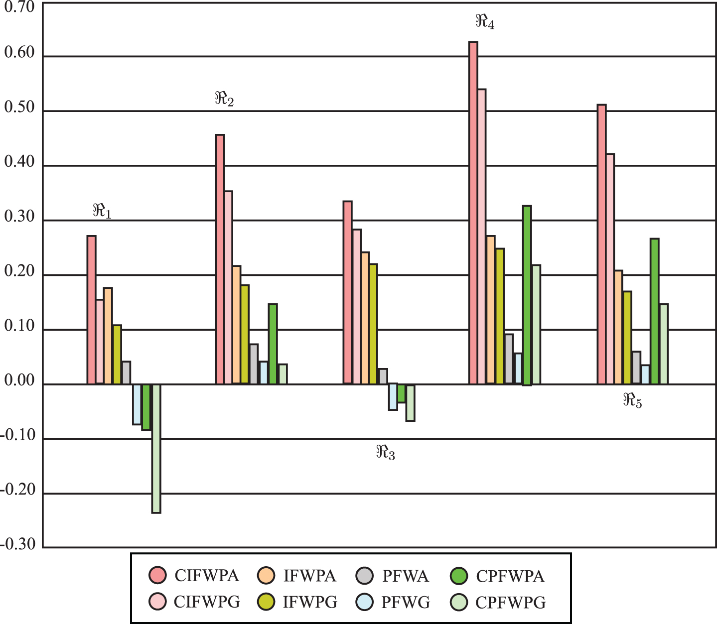
In this section, we analyze the comparison of presented model with some existing models. The existing models which we have chosen for the comparison are based on the operators defined under IFS [46], CIFS [36] and PFS [43]. For IFS and PFS, we put the phase term and neutral membership zero related to each CPFN of given data. To compare the proposed model with CIFS, we take complex grade of neutral membership of each CPFN zero. Then the results based on given information are exhibited by Table 6.

Table 6
Comparison with some existing models

Existing models Score values Ranking

$R_{1}$ $R_{2}$ $R_{3}$ $R_{4}$ $R_{5}$

IFWPA [46] 0.1805 0.2194 0.2421 0.2713 0.2028 $R_{4} ≻ R_{3} ≻ R_{2} ≻ R_{5} ≻ R_{1}$

IFWPG [46] 0.1021 0.1844 0.2132 0.2275 0.1762 $R_{4} ≻ R_{3} ≻ R_{2} ≻ R_{5} ≻ R_{1}$

CIFWPA [36] 0.2825 0.4564 0.3279 0.6240 0.5156 $R_{4} ≻ R_{5} ≻ R_{2} ≻ R_{3} ≻ R_{1}$

CIFWPG [36] 0.1585 0.3703 0.2920 0.5356 0.4261 $R_{4} ≻ R_{5} ≻ R_{2} ≻ R_{3} ≻ R_{1}$

PFWA [43] 0.0152 0.0704 0.0006 0.0983 0.0539 $R_{4} ≻ R_{2} ≻ R_{5} ≻ R_{1} ≻ R_{3}$

PFWG [43] -0.0756 0.0076 -0.0380 0.0364 0.0201 $R_{4} ≻ R_{5} ≻ R_{2} ≻ R_{3} ≻ R_{1}$

Existing models	Score values					Ranking
IFWPA [46]	0.1805	0.2194	0.2421	0.2713	0.2028	$R_{4} ≻ R_{3} ≻ R_{2} ≻ R_{5} ≻ R_{1}$
IFWPG [46]	0.1021	0.1844	0.2132	0.2275	0.1762	$R_{4} ≻ R_{3} ≻ R_{2} ≻ R_{5} ≻ R_{1}$
CIFWPA [36]	0.2825	0.4564	0.3279	0.6240	0.5156	$R_{4} ≻ R_{5} ≻ R_{2} ≻ R_{3} ≻ R_{1}$
CIFWPG [36]	0.1585	0.3703	0.2920	0.5356	0.4261	$R_{4} ≻ R_{5} ≻ R_{2} ≻ R_{3} ≻ R_{1}$
PFWA [43]	0.0152	0.0704	0.0006	0.0983	0.0539	$R_{4} ≻ R_{2} ≻ R_{5} ≻ R_{1} ≻ R_{3}$
PFWG [43]	-0.0756	0.0076	-0.0380	0.0364	0.0201	$R_{4} ≻ R_{5} ≻ R_{2} ≻ R_{3} ≻ R_{1}$

Based on the calculations, presented by Table 6 $R_{4}$ is the optimal alternative which shows that the given model is logical and reliable. Due to the fluctuating circumstances of choices, a slight difference appears in the ranking of alternatives, i.e., the aggregated results are obtained either with different operators or under different environments.

Despite the fact that the best alternative is same for all discussed techniques examined by the MCDM method, the CPFWP operators are superior than the existing models. Because the CPFWP operators can exhibit two dimensional information and the generalized form of IFS, CIFS and PFS.

The comparative analysis is graphically shown in the Fig. 2

Fig. 2

Comparison of proposed and existing models.

7.1 Merits of proposed technique

The preeminence and some advantages of the proposed technique, based on the comparative study are illustrated in the following aspect.

The dominance of CPFSs rely on the ability of exhibiting two dimensional phenomenon. This ability makes these sets more effective as these sets can possess more relevant information about an object during a strategy. Therefore, CPFS is the most generalized form of CIFS [8] and PFS [16] which can be illustrated as follows:

CIFSs can deal with two dimensional data but only exhibit the information about the membership and non-membership degrees. PFS has ability to discuss the membership, non-membership as well as neutral membership degree but it fails to handle the periodicity due to absence of phase term. The CPFS not only possesses the knowledge about membership, neutral membership, non-membership and hesitancy values, but also deals with imprecision and periodicity simultaneously. In this manner, the proposed aggregation technique under CPFSs is more generalized than the other existing models.

Furthermore, CIFS [8] and PFS [16] are the special cases of CPFS. Because, the CPFS can be converted either into the CIFS or PFS by taking neutral membership or phase term zero, respectively. Therefore, the aggregation methods described in [18 , 43] can be easily explained under CPFSs environment but the proposed method can not be expressed under the existing environments.

Most importantly, the distinct and noticeable feature of the presented MCDM technique is to explore the pertinent and valid information for the appraisal of alternatives with minimum data loss. The PA technique makes it more easier and comfortable for the decision maker(s) to develop the interdependent interactions among the arguments for appraisal of optimal result as these operators have capacity to display the relationship of contentions and above all the inclinations fortify up one another during the aggregation cycle. Therefore, the presented method is more reliable and convenient for handling the MCDM issues.

8 Conclusion

The CPFS is a generalization of PFS and CIFS as the PFS can not deal with two-dimensional data whereas, CIFS lacks the information about an item viable. Fundamentally, the expansion of neutral membership degree to the meaning of CIFS fortifies the significance of set which gives more angles to know about an object under consideration. The membership degrees of a CPFS are complex valued consisting of amplitude and phase terms which make CPFS more effective and influential mechanism to deal with the imprecision and periodicity of data, simultaneously, to solve the MCDM issues and provide many different ways to the decision expert for making the best choice of desired alternatives. In this research, we present a novel concept of CPFSs and define the basic properties and some operational laws which are helpful to understand the CPFSs. We have proposed an aggregation technique namely; complex picture fuzzy power averaging and geometric operators, including weighted and ordered weighted aggregation techniques and explained their importance and authenticity by proposing a MCDM model, based on an algorithm and a descriptive example. The analysis of proposed and existing models has been done to illustrate the superiority and consistency of presented approach. This analysis has proven our model more general and flexible for decision makers to access an alternative in the most desirable environment. Finally, we have expressed the merits of presented model. In future research, we extend our work to Prioritized and Einstein aggregation operators under CPFSs environment.

Conflict of Interest: The authors declare no conflict of interest.

References

Akram

and Bashir

, Complex fuzzy ordered weighted quadratic averaging operators, Granular Computing (2020). DOI:10.1007/s41066-020-00213-7

Akram

, Bashir

and Garg

, Decision-making model under complex picture fuzzy Hamacher aggregation operators, Computational and Applied Mathematics 39(2020), https://doi.org/10.1007/s40314-020-01251-2.

Akram

, Dudek

W.A.

and Dar

J.M.

, Pythagorean Dombi fuzzy aggregation operators with application in multi-criteria decision-making, International Journal of Intelligent Systems 34 (2019), 3000–3019.

Akram

, Dudek

W.A.

and Ilyas

, Group decision making based on Pythagorean fuzzy TOPSIS method, International Journal of Intelligent Systems 34 (2019), 1455–1475.

Akram

, Garg

and Zahid

, Extensions of ELECTRE-I and TOPSIS methods for group decisionmaking under complex Pythagorean fuzzy environment, Iranian Journal of Fuzzy Systems 17(5) (2020), 147–164.

Akram

, Khan

and Saeid

A.B.

, Complex Pythagorean Dombi fuzzy operators using aggregation operators and their decision-making, Expert Systems (2020), https://doi.org/10.1111/exsy.12626.

Akram

, Peng

and Sattar

, Multi-criteria decision-making model using complex Pythagorean fuzzy Yager aggregation operators. Arabian Journal for Science and Engineering, (2020). https://doi.org/10.1007/s13369-020-04864-1.

Alkouri

and Salleh

, Complex intuitionistic fuzzy sets, 2nd international conference on fundamental and applied sciences 1482(2012), 464–470.

Atanassov

, Intuitionistic fuzzy sets, Fuzzy Sets and Systems 20(1) (1986), 87–96.

10.

, Dai

and Hu

, Complex fuzzy geometric aggregation operators, Symmetry 10 (2018), 251.

11.

, Dai

, Hu

and Li

, Complex fuzzy arithmetic aggregation operators, Journal of Intelligent and Fuzzy Systems 36(3) (2019), 2765–2771.

12.

Chen

S.M.

and Chang

C.H.

, Fuzzy multi-attribute decision making based on transformation techniques of intuitionistic fuzzy values and intuitionistic fuzzy geometric averaging operators, Information Sciences (2016), 352–353, 133–149.

13.

Chen

S.M.

and Tan

J.M.

, Handling multi-criteria fuzzy decision-making problems based on vague set theory, Fuzzy Sets and Systems 167 (1994), 163–172.

14.

Chiclana

, Herrera

and Herrera-Viedma

, The ordered weighted geometric operator, Properties and application. In: Proc of 8th Int Conf on Information Processing and Management of Uncertainty in Knowledgebased Systems, Madrid, (2000), 985–991.

15.

Cuong

, Picture fuzzy sets-first results, Neuro-Fuzzy Systems with Applications, Institute of Mathematics, Hanoi, (2013).

16.

Cuong

B.C.

and Kreinovich

, Picture Fuzzy Sets-a new concept for computational intelligence problems. In 2013 Third World Congress on Information and Communication Technologies (WICT 2013) (2013), 1–6.

17.

Figueira

, Greco

and Ehrgott

, Multiple criteria decision analysis, Springer New York, (2016).

18.

Garg

, Some picture fuzzy aggregation operators and their applications to multi-criteria decision making, Arabian Journal for Science and Engineering 42(12) (2017), 5275–5290.

19.

Garg

, Distance and similarity measure for intuitionistic multiplicative preference relation and its application, International Journal for Uncertainty Quantification 7(2) (2017), 117–133.

20.

Garg

and Rani

, Some generalized complex intuitionistic fuzzy aggregation operators and their application to multi-criteria decision-making process, Arabian Journal for Science and Engineering 44(3) (2019), 2679–2698.

21.

Khan

, Abdullah

and Ashraf

, Picture fuzzy aggregation information based on Einstein operations and their application in decision making, Mathematical Sciences 13(3) (2019), 213–229.

22.

Lin

, Li

and Chen

, Linguistic q-rung orthopair fuzzy sets and their interactional partitioned Heronian mean aggregation operators, International Journal of Intelligent Systems 35(2) (2020), 217–249.

23.

Lin

, Huang

and Xu

, MULTIMOORA based MCDM model for site selection of car sharing station under picture fuzzy environment, Sustainable Cities and Society 53 (2020), 101873.

24.

Lin

, Wei

, Xu

and Chen

, Multi-attribute group decision-making based on linguistic Pythagorean fuzzy interaction partitioned bonferroni mean aggregation operators, Complexity (2018). https://doi.org/10.1155/2018/9531064.

25.

Lin

, Xu

, Lin

and Chen

, Determine OWA operator weights using kernel density estimation, Economic Research-Ekonomska Istra đ ivanja 33(1) (2020), 1441–1464.

26.

Liu

, Akram

and Sattar

, Extensions Of prioritized weighted aggregation operators for decisionmaking under complex q-rung orthopair fuzzy information, Journal of Intelligent and Fuzzy Systems (2020). DOI:10.3233/JIFS-200789

27.

Liu

, Chen

S.M.

and Wang

, Multi-attribute group decision making based on intuitionistic fuzzy partitioned Maclaurin symmetric mean operators, Information Sciences 512 (2020), 830–854.

28.

Liu

, Shahzadi

and Akram

, Specific types of q-rung picture fuzzy Yager aggregation operators for decision-making, International Journal of Computational Intelligence Systems 13(1) (2020), 1072–1091.

29.

Liu

, Liu

and Chen

S.M.

, Some intuitionistic fuzzy Dombi Bonferroni mean operators and their application to multi-attribute group decision making, Journal of the Operational Research Society 69(1) (2018), 1–24.

30.

Liu

H.W.

and Wang

G.J.

, Multi-criteria decision-making methods based on intuitionistic fuzzy sets, European Journal of Operational Research 179(1) (2007), 220–233.

31.

Liu

, Wang

and Liu

, Multiple attribute group decision making based on q-rung orthopair fuzzy Heronian mean operators, International Journal of Intelligent Systems 33(12) (2018), 2341–2363.

32.

Liu

, Wang

, Li

, Zhao

and Liu

, q-rung orthopair fuzzy multiple attribute group decisionmaking method based on normalized bidirectional projection model and generalized knowledgebased entropy measure, Journal of Ambient Intelligence and Humanized Computing (2020). https://doi.org/10.1007/s12652-020-02433-w.

33.

Pasi

and Yager

R.R.

, Modelling the concept of majority opinion in group decision making, Information Sciences 176 (2006), 390–414.

34.

Ramot

, Friedman

, Langholz

and Kandel

, Complex fuzzy logic, IEEE Transactions on Fuzzy Systems 11(4) (2003), 450–461.

35.

Ramot

, Milo

, Friedman

and Kandel

, Complex fuzzy sets, IEEE Transactions on Fuzzy Systems 10(2) (2002), 171–186.

36.

Rani

and Garg

, Complex intuitionistic fuzzy power aggregation operators and their applications in multi-criteria decision-making, Expert System (2018).

37.

Rani

and Garg

, Distance measures between the complex intuitionistic fuzzy sets and its applications to the decision-making process, International Journal for Uncertainty Quantification 7(5) (2017), 423–439.

38.

Shahzadi

, Akram

and Al-Kenani

A.N.

, Decision making approach under Pythagorean fuzzy Yager weighted operators, Mathematics 8(1) (2020), 70.

39.

Shumaiza , Akram

, Al-Kenani

A.N.

and Alcantud

J.C.R.

, Group Decision-Making Based on the VIKOR Method with Trapezoidal Bipolar Fuzzy Information, Symmetry 11(10) (2019), 1313.

40.

Singh

and Garg

, Distance measures between type-2 intuitionistic fuzzy sets and their application to multicriteria decision-making process, Applied Intelligence 46(4) (2017), 788–799.

41.

Wang

and Triantaphyllou

, Ranking irregularities when evaluating alternatives by using some ELECTRE methods, Omega 36 (2008), 45–63.

42.

Waseem

, Akram

and Alcantud

J.C.R.

, Multi-attribute decision-making based on m-polar fuzzy Hamacher aggregation operators, Symmetry 11(12) (2019), 1498.

43.

Wei

G.W.

, Picture fuzzy aggregation operators and their application to multiple attribute decision making, Journal of Intelligent and Fuzzy Systems 33(2) (2017), 713–724.

44.

Wei

, Zhao

, Wang

and Lin

, Fuzzy power aggregation operators and their application to multiple attribute group decision making, Technological and Economic Development of Economy 19(3) (2013), 377–396.

45.

, Intuitionistic fuzzy aggregation operators, IEEE Transactions on Fuzzy Systems 15(6) (2007), 1179–1187.

46.

, Approaches to multiple attribute group decision making based on intuitionistic fuzzy power aggregation operators, Knowledge-Based Systems 24(6) (2011), 749–760.

47.

Z.S.

and Yager

R.R.

, Some geometric aggregation operators based on intuitionistic fuzzy sets, International Journal of General Systems 35(2006), 417–433.

48.

and Yager

R.R.

, Power-geometric operators and their use in group decision making, IEEE Transactions on Fuzzy Systems 18(1) (2010), 94–105.

49.

Yager

R.R.

, Aggregation operators and fuzzy systems modeling, Fuzzy Sets and Systems 67(2) (1994), 129–145.

50.

Yager

R.R.

, The power average operator, IEEE Systems, Man, and Cybernetics Society 31(6) (2001), 724–731.

51.

Yager

R.R.

, On ordered weighted averaging aggregation operators in multicriteria decision making, IEEE Transactions on Systems Man and Cybernetics 18(1) (1988), 183–190.

52.

, Intuitionistic fuzzy hybrid arithmetic and geometric aggregation operators for the decisionmaking of mechanical design schemes, Applied Intelligence 47 (2017), 743–751.

53.

Zadeh

L.A.

, Fuzzy sets, Information and Control 8(3) (1965), 338–356.

54.

Zhang

G.T.

, Dillon

, Cai

K.Y.

, Ma

and Lu

, Operation properties and ä-equalities of complex fuzzy sets, International Journal of Approximate Reasoning 50 (2009), 1227–1249.