A microbial kinetic optimization approach

Abstract

In order to solve some optimization problems with many local optimal solutions, a microbial dynamic optimization (MDO) algorithm is proposed by the kinetic theory of hybrid food chain microorganism cultivation with time delay. In this algorithm, it is assumed that multiple microbial populations are cultivated in a culture system. The growth of microbial populations is not only affected by the flow of culture fluid injected into the culture system, the concentration of nutrients and harmful substances, but also by the interaction between the populations. The influence of culture medium which is injected regularly will suddenly increase the concentration of nutrients and toxic substances, it will suddenly increase the impact on the population. These characteristics are used to construct absorption operators, grabbing operators, hybrid operators, and toxin operators; the global optimal solution of the optimization problem can be quickly solved by these operators and the population growth changes. The simulation experiment results show that the MDO algorithm has certain advantages for solving optimization problems with higher dimensions.

Keywords

Swarm intelligence optimization algorithm microbial culture kinetics microbial population microbial dynamics optimization (MDO)

1 Introduction

In engineering, there are many optimization problems with a large number of local optimal solutions, and in many cases, the mathematical expressions of the objective function and constraint conditions of these optimization problems have no restrictions, traditional optimization algorithms cannot solve such optimization problems. At present, the method to solve such optimization problems is swarm intelligence optimization algorithm [1 –5]. Different from the traditional optimization algorithm, when the swarm intelligence optimization algorithm solves an optimization problem, it uses a number of trial solutions to perform evolutionary calculations at the same time. This “group attack” method can solve some very difficult optimization problems [6 –11]. However, there is no swarm intelligence optimization algorithm that can solve all types of optimization problems [12]. In the swarm intelligence optimization algorithm, each trial solution is compared to an individual with biological characteristics. Some special biological evolution scenarios are converted into the logical structure of the swarm intelligence algorithm. The interaction between the biological individuals active in the scenario is used to construct the evolution operator of individual organisms [13].

Population dynamics is a mathematical theory that reflects the interaction between biological populations [14]. Population dynamics contains many branches, and each branch has the potential to transform into a swarm intelligence algorithm. Based on the Lotka-Volterra model, a special population dynamics optimization algorithm is constructed [15]. The algorithm uses the interaction relationship between the three populations, namely the mutually beneficial coexistence relationship, the competition relationship, and the predator-prey relationship to construct an evolution operator. The evolution characteristics of all operators can ensure that the algorithm has global convergence. By using population dynamics theory, a population dynamics-based optimization (PDO) algorithm is constructed [16]. The algorithm uses predation-being, mutual benefit, fusion, competition, mutation, and selection between any two groups to construct the evolution strategy of the population. An improved PDO algorithm is proposed based on the theory of population dynamics [17]. This algorithm is used to quickly determine the best guide path for eliminating concentrated mine dust from multiple points underground. Another improved PDO algorithm is proposed by using the predation-being theory in population dynamics [18], it can quickly determine the best installation positions of underground mine dust collection stations, underground fans and ventilation structures. In a multi-agent framework, distributed optimization problems are generally described as the minimization of a global objective function, where each agent can get information only from a neighborhood defined by a network topology. To solve the problem, an information-constrained strategy was presented based on population dynamics [19], where payoff functions and tasks are assigned to each node in a connected graph. Searching for the optimal subset of features is known as a challenging problem in feature selection process. To deal with the difficulties involved in this problem, a robust and reliable optimization algorithm is required. Grasshopper Optimization Algorithm (GOA) is employed as a search strategy to design a wrapper-based feature selection method [20]. A new mutation strategy and a bionic bi-population structure are incorporated, a new differential evolution variant is used to enhance the overall performance of the canonical differential evolution algorithm [21]. The biological activity scenarios that have been proposed for swarm intelligence optimization algorithms are very simple and have weak mathematical foundations, such as genetic algorithm, ant colony algorithm, biogeographic algorithm, and bee colony algorithm. Some swarm intelligence optimization algorithms do not even have biological activity scenarios, such as particle swarm algorithm and differential evolution algorithm. If a swarm intelligence optimization algorithm has a clear and vivid biological activity scene, and the scene can be accurately described by mathematical theory, then this scene is extremely conducive to constructing a swarm intelligence optimization algorithm, because the swarm intelligence optimization algorithm is based on good mathematics, its performance is easy to be analyzed.

Microbial culture is the use of a culture room to cultivate one or more microbial populations. Microbial culture kinetics is a mathematical theory that studies the interaction and continuous evolution of microbial populations in a culture room under human control. Microbial culture dynamics is one of the branch of population dynamics [14]. In order to use some special properties of microbial culture dynamics to construct a high-performance swarm intelligence optimization algorithm, in this paper, a time-lag-affected hybrid food chain microbial pulse culture dynamics model is used to construct a microbial dynamics optimization algorithm (microbial dynamics optimization, MDO). In this algorithm, a design idea is adopted, it is different from the existing population dynamics optimization algorithm, and a microbial culture dynamics model is proposed and transformed into a general method, some optimization problems can be solved. The constructed operator can fully reflect the influence of the toxic substances in the culture system and the culture fluid on the microbial population and the interaction relationship between the microbial populations, thus the basic idea of the microbial culture dynamics theory is reflected. The MDO algorithm can converge globally and has certain advantages for solving optimization problems with higher dimensions.

2 Basic principles of the algorithm

2.1 Scene design of MDO algorithm

Suppose that there are N microbial populations living in the microbial culture system E, namely P₁, P₂,...,P_i,...,P_N; each population not only feeds on the culture fluid in E, but also feeds the other K populations in E for food. In the process of microbial cultivation, the prepared fresh medium is periodically injected into E; at the same time, the useless medium is continuously removed from E; the medium absorbed by the microbial population will not be converted into immediately new microbial population, in other words, there is a period of time in the process of transforming from the culture fluid to the microbial population; as the culture fluid is injected, harmful substances are also injected. In order to control the destructive effects of harmful substances on the population, it is necessary to continuously assess the degree of damage to the population by the harmful substances. The operation of the culture system can be achieved by differently controlling two factors: one is the concentration S of nutrients in the culture solution; the other is the flow rate Q of the culture solution. Changes in the concentration of S will cause changes in the growth of microbial populations.

The characteristics of the microbial population P_i can be represented by P_i = {f_i,1,f_i,2,...,f_i,n}, where f_i,j are the characteristics j of P_i, n is the total number of characteristics of each population, i = 1∼N, j = 1∼n; the influence of the nutrient concentration of the culture medium in E on the population P_i is reflected in the random influence on the characteristics of the population P_i.

Suppose the optimization model of the required solution is Equation (1): ${\begin{matrix} min f (X) \\ X \in H \subset R^{n} \end{matrix}$ (1)

In the formula (1), Rⁿ is the n-dimensional Euclidean space, H is the search space; f(X) is the objective function; X is the n-dimensional solution vector, X = (x₁,x₂,...,x_i,...,x_n), and x_i is the solution component. N initial solutions are selected arbitrarily in H, namely H = {X₁,X₂,...,X_N}, where X_i = (x_i,1,x_i,2,...,x_i,n), i = 1∼N; culture system E corresponds to the search space H. The N initial solutions of the optimization model correspond to the N microbial populations in E, that is, X_i corresponds to P_i one to one; more precisely, the variables x_i,j of X_i correspond to the characteristics f_i,j of P_i one to one.

In summary, the initial solution and the microbial population are equivalent concepts and will not be distinguished later. After P_i takes in nutrients, its growth state will change. This change is projected to H, it is equivalent to transferring the initial solution Xi from the spatial position a to b. A spatial location is called a state and is described by its subscript.

Assuming that the current state of P_i is c, this is equivalent to the position X_c in H. If P_i evolves from state c to state d after taking in nutrients, this is equivalent to jumping from position X_c to position X_d in H. Calculate according to formula (1), if f(X_c) > f(X_d), indicating that position X_c is better than position X_d, then P_i is considered strong. Conversely, if f(X_c)≤f(X_d), indicating that the position X_d is worse than the position X_c, or there is no difference (because f(X_c) = f(X_d)), then P_i is considered weak. The strong population can continue to grow with a higher probability, while the weak population may not grow anymore.

The strength of P_i can be expressed by the microbial growth index (MGI). A good quality solution corresponds to a population with a higher MGI index, that is, a strong population. A poor quality solution corresponds to a population with a lower MGI index, that is, a weak population. For formula (1), the MGI index of Pi is calculated according to formula (2): $MGI (X_{i}) = {\begin{matrix} \frac{1}{1 + f (X_{i})}, if f (X_{i}) > 0 \\ 1 + | f (X_{i}) |, if f (X_{i}) ⩽ 0 \end{matrix}, i = 1 \sim N$ (2)

In E, the biological intelligence characteristics of microbial cultivation are reflected in the following aspects:

Various groups have mutual influence due to competition for culture solution. Such influence will be reflected in the random interaction between certain characteristics of the group. This is the “competitive intelligent characteristic”.

When a population feeds on other populations, some characteristics of the eaten populations will be incorporated into some characteristics of the population, which is the “smart characteristic of eating”.

The evolution of any population is obtained by continuously learning from other strong populations, which is the “intelligent feature of learning”.

The characteristics of biological intelligence cultivated by microorganisms are finally embodied in the form of biological evolution operators. The interaction between all microbial populations is projected to H in Equation (1), that is, there is an interaction between the solution vectors.

The MDO algorithm uses such strategies to solve the global optimal solution of Equation (1).

2.2 Microbial culture kinetic model

Suppose there are N species of microorganism populations in the culture system E, and each population feeds on the culture fluid and L other populations in E as food. In addition, toxic substances will poison all populations. At period t, the concentration of the population P_i is y_i(t), y_i(t) ≥0, i = 1∼N; the culture fluid flows into E at a flow rate Q, where the concentration of nutrients is S₀. This culture system has a time-lag effect on the mixed food chain microbial pulse culture dynamic model, as shown in formula (3) [14]: ${\begin{matrix} \frac{dS (t)}{dt} = - QS (t) - \sum_{i = 1}^{N} \frac{c_{0} μ_{0} S (t)}{K_{0} + S (t)} y_{i} (t), t \neq kT \\ \frac{{dy}_{i} (t)}{dt} = e^{- Q τ} \frac{μ_{0} S (t - τ)}{K_{0} + S (t - τ)} y_{i} (t + τ) - \sum_{s \in MS (t)} \frac{α_{0} γ_{0} Y_{S} (t)}{W_{0} + Y_{S} (t)} - (Q + rc (t)) y_{i} (t), i = 1, 2, \dots, N, t \neq kT \\ \frac{dc (t)}{dt} = - Qc (t), t \neq kT \\ S (t^{+}) = S (t) + S_{0}, t = kT \\ y_{i} (t^{+}) = y_{i} (t), i = 1, 2, \dots, N, t = kT \\ c (t^{+}) = c (t) + q_{0}, t = kT \\ S (0^{+}) ⩾ 0; y_{i} (0^{+}) ⩾ 0, i = 1, 2, \dots, N, c (t^{+}) ⩾ 0_{,} t = kT \end{matrix}$ (3)

In the formula (3), S(t) represents the nutrient concentration of the culture solution at period t; μ ₀ represents the relative growth coefficient of the population; C₀ represents the consumption rate of the culture solution by the population; MS(t) represents a collection of numbers of the K populations captured by the population P_i at period t; K₀, α₀, γ₀, W₀ represent constants related to population growth; y_i(t) represents the concentration of the population P_i at period t; c(t) represents the concentration of harmful substances, c(t)≥0; q₀ represents the quantity of harmful substances input in each culture medium feeding period; r represents the reduction rate of the population due to poisoning and death due to harmful substances, r > 0; T represents the feeding period of the culture fluid; τ represents the lag time of the transformation of the culture fluid to the microbial population; t⁺ is the time when the culture medium is put into use; k represents a positive integer, k≥1.

At period t, the proportion r_i(t) of the population P_i is calculated according to formula (4): $r_{i} (t) = \frac{y_{i} (t)}{\sum_{s = 1}^{N} y_{s} (t)}, i = 1 \sim N$ (4)

The larger the proportion r_i(t) of the population P_i, the greater the chance of being preyed by other populations. The values of the time t parameters C₀, Q, K₀, S₀, α₀, μ₀, r, γ₀, W₀, and q₀ are respectively C^t₀, Q^t, K^t₀, S^t₀, α^t₀, μ^t₀, r^t, γ^t₀, W^t₀, q^t₀. In order to facilitate the calculation, the formula (3) is changed to a discrete recursive form, with the following formula: ${\begin{matrix} S (t + 1) = S (t) - Q^{t} S (t) - \sum_{i = 1}^{N} \frac{c_{0}^{t} μ_{0}^{t} S (t)}{K_{0} + S (t)} y_{i} (t), t \neq kT \\ c (t + 1) = c (t) - Q^{t} c (t), t \neq kT \end{matrix}$ (5)

$\begin{matrix} y_{i} (t + 1) = y_{i} (t) + e^{- Q^{t} τ} \frac{c_{0}^{t} μ_{0}^{t} S (t - τ)}{K_{0} + S (t - τ)} y_{i} (t - τ) \\ - \sum_{s \in MS (t)} \frac{α_{0}^{t} γ_{0}^{t} y_{s} (t)}{W_{0}^{t} + y_{s} (t)} - (Q^{t} + r^{t} c (t)) y_{i} (t), \\ i = 1, 2, \dots, N, t \neq kT \end{matrix}$ (6) ${\begin{matrix} S (t + 1) = S (t) + S_{0}^{t}, t = kT \\ c (t + 1) = c (t) + q_{0}^{t}, t = kT \end{matrix}$ (7) $y_{i} (t + 1) = y_{i} (t), i = 1, 2, \dots, N, t = kT$ (8)

Refer to Table 1 for the meaning of each parameter and its value restriction conditions in formula (5) and formula (6).

Table 1

Strategy of taking value for parameters of microbial dynamics model

Parameter name	Value strategy	Parameter name	Value strategy
Q^t	Qt = Rand(1,100)	r^t	r^t = Rand(0.1,0.3)
S^t₀	S^t₀ = Rand(0.1,0.9)	q^t₀	q^t₀ = Rand(1.2,3.5)
C^t₀	C^t₀ = Rand(0.4,0.6)	τ	τ≥0
K^t₀	K^t₀ = Rand(0.3,0.7)	T	T≥1
μ ^t ₀	μ ^t ₀ = Rand(1.1,1.9)	M	M≥1
α ^t ₀	α ^t ₀ = Rand(0.3,0.7)	L	L≥1
γ ^t ₀	γ ^t ₀ = Rand(0.3,0.7)	K	K = 2∼10
W^t₀	W^t₀ = Rand(0.3,0.7)

In Table 1, Rand(A,B) means generating a random number that obeys a uniform distribution in the interval [A,B]. A and B are constants, and A≤B.

2.3 Generation strategy of characteristic microbial population collection

At period t, suppose the current population is P_i, the generation strategy of the characteristic microbial population set is as follows:

Generate the set MS(t) of the eaten population. At period t, the population P_i feeds on another K populations, that is, K populations are randomly selected from N-1 populations with {r₁ (t), r₂ (t),...,r_N (t)} as the probability distribution (But P_i cannot be selected), these populations form a set MS(t), let us set MS (t) = {i₁,i₂, ... ,i_k, ... ,i_K}, where i_k is the number of the population P_ik, k = 1∼K.

Generate aggregates FM^t, GM^t, and HM^t of 30%, 20%, and 10% strong populations respectively. At period t, L populations are randomly selected from N populations. The MGI index of these populations is 30% higher than the current population P_i, forming a set FM^t = {X_s1 (t),X_s2 (t),...,X_sL (t)}, where s₁, s₂,...,s_L are the numbers of these selected populations. Then randomly select L populations from the remaining N-L populations. The MGI index of these populations is 20% higher than the current population P_i, forming a set GM^T = {X_g1 (t), X_g2 (t),...,X_gL (t)}, Where g₁, g₂,...,g_L are the numbers of these selected populations; finally L populations are randomly selected from the remaining N-2L populations, and the MGI index of these populations is 10% higher than the current population P_i, forming a set HM^t = {X_h1 (t),X_h2 (t),...,X_hL (t)}, where h₁,h₂,...,h_L are the numbers of these selected populations.

Generate 15% AS^t, BS^t, CS^t of strong population, weak population, and ordinary population respectively. At period t, L strong populations are randomly selected from N populations, and their MGI index is higher than 15% of the current population P_i, forming a strong population set AS^t = {X_a1 (t),X_a2 (t),...,X_aL (t)}, where a₁, a₂, ... , a_L are the numbers of these selected populations; then L weak populations are randomly selected from N populations, whose MGI index is lower than 15% of the current population P_i, forming a weak population set BS^t = {X_b1 (t), X_b2 (t),...,X_bL (t)}, where b₁, b₂,..., b_L are the numbers of these selected populations. Finally, L common populations are selected randomly from the remaining N-2L populations, their MGI index has nothing to do with the MGI index of the current population P_i, forming a common population set CS^t = {X_c1 (t),X_c2 (t),...,X_cL (t)}, where c₁,c₂,..., c_L is the number of these selected populations.

2.4 Design of microbial population evolution operator

The MDO algorithm uses the microbial cultivation dynamics model formula (3) to construct the evolution operator, so as to realize the information exchange between the cultivation system and the population and between the population and the population, and then realize the search of the search space H of the formula (1).

(1) Absorption operator. The absorption operator describes the nutrient supply relationship between the population P_i and the other K populations. Pass a randomly selected feature f_s,j,s∈MS(t) of the eaten population in the set MS(t) to the current population P_i, so that the population P_i can grow: $v_{i, j} (t + 1) = η_{i} x_{i, j} (t) + \sum_{s \in MS (t)} β_{s} x_{s, j} (t)$ (9)

In formula (9), x_s,j(t) represents the state value of the feature j of the population P_s at period t, that is, the value of the variable x_s,j at period t; v_i,j(t + 1) represents the state value of the feature j of the population P_i at period t + 1, that is, the value of the variable x_i,j in the period t + 1; Take β _s = Rand(-0.95,0.95), η _i = Rand(0.45,0.65).

(2) Snap operator. The snap operator describes that a population grabs the dominant characteristics of other populations to make it stronger. Let the characteristics f_sl,j, s_l∈ {h₁,h₂, ... ,h_L; g₁,g₂, ... ,g_L; s₁,s₂, ... ,s_L} correspond to the characteristics of the 3 L strong populations in FM^t, GM^t and HM^t, f_sl,j The value is passed to the characteristic f_i,j of the population P_i, making P_i strong. Assuming that the current population is P_i and the feature for dominance grabbing is f_i,j, then there is formula (10): $v_{i, j} (t + 1) = {\begin{matrix} {\begin{matrix} 0.9 x_{d_{1, j}} (t) + 0.5 (x_{d_{2, j}} (t) - x_{d_{3, j}} (t)), | {FM}^{t} | > 0, 0 < Rand (0, 1) ⩽ \frac{1}{2} \\ x_{i, j} (t), | {FM}^{t} | = 0, 0 < Rand (0, 1) ⩽ \frac{1}{2} \end{matrix} \\ {\begin{matrix} 0.9 x_{e_{1, j}} (t) + 0.5 (x_{e_{2, j}} (t) - x_{e_{3, j}} (t)), | {GM}^{t} | > 0, \frac{1}{2} < Rand (0, 1) ⩽ \frac{3}{4} \\ x_{i, j} (t), | {GM}^{t} | = 0, \frac{1}{2} < Rand (0, 1) ⩽ \frac{3}{4} \end{matrix} \\ {\begin{matrix} 0.9 x_{p_{1, j}} (t) + 0.5 (x_{p_{2, j}} (t) - x_{p_{3, j}} (t)), | {HM}^{t} | > 0, \frac{3}{4} < Rand (0, 1) ⩽ 1 \\ x_{i, j} (t), | {HM}^{t} | = 0, \frac{3}{4} < Rand (0, 1) ⩽ 1 \end{matrix} \end{matrix}$ (10)

In the formula (10), d₁, d₂, d₃, e₁, e₂, e₃, p₁, p₂, and p₃ are randomly selected from the sets FM^t, GM^t, and HM^t respectively, and they satisfy d₁≠d₂ ≠d₃, e₁≠e₂≠e₃, p₁≠p₂≠p₃.

(3) Hybrid operator. The confounding operator describes the interaction between the population and the population. For the current population P_i, the state value of which the features f_sl,j, s_l∈{a₁,a₂, ... ,a_L; b₁,b₂, ... ,b_L;c₁,c₂, ... ,c_L} of the 3 L populations in AS^t, BS^t, CS^t correspond to is passed to the characteristic f_i,j of the population P_i after being mixed and fused, then there is formula (11): $\begin{matrix} v_{i, j} (t + 1) = \\ {\begin{matrix} λ_{i} x_{i, j} (t) + \sum_{s \in {AS}^{t}} ρ_{s} x_{s, j} (t), j = 1 \sim n, 0 < Rand (0, 1) ⩽ \frac{1}{6} \\ λ_{i} x_{i, j} (t) + \sum_{s \in {AS}^{t}} ρ_{s} x_{s, j} (t), j = 1 \sim n, \frac{1}{6} < Rand (0, 1) ⩽ \frac{1}{3} \\ λ_{i} x_{i, j} (t) + \sum_{s \in {BS}^{t}} ρ_{s} x_{s, j} (t), j = 1 \sim n, \frac{1}{3} < Rand (0, 1) ⩽ \frac{1}{2} \\ λ_{i} x_{i, j} (t) + \sum_{s \in {BS}^{t}} ρ_{s} x_{s, j} (t), j = 1 \sim n, \frac{1}{2} < Rand (0, 1) ⩽ \frac{2}{3} \\ λ_{i} x_{i, j} (t) + \sum_{s \in {AS}^{t}} ρ_{s} x_{s, j} (t), j = 1 \sim n, \frac{2}{3} < Rand (0, 1) ⩽ \frac{5}{6} \\ λ_{i} x_{i, j} (t) + \sum_{s \in {AS}^{t}} ρ_{s} x_{s, j} (t), j = 1 \sim n, \frac{5}{6} < Rand (0, 1) ⩽ 1 \\ λ_{i} = Rand (0.65, 0.85), ρ_{s} = Rand (0.75, 0.85) \end{matrix} \end{matrix}$ (11)

(4) Toxin operator. The toxin operator describes the toxic effects of toxic substances in the external system on microorganisms, and the toxic effects can be transmitted between microbial populations. For the current population P_i, there is formula (12): $v_{i, j} (t + 1) = c (t) (x_{g_{1}, j} (t) + x_{g_{2}, j} (t)) + (1 - c (t)) x_{g_{3}, j} (t)$ (12)

In formula (12), g₁, g₂, g₃ are randomly selected from {1, 2, . . . , N}, and they satisfy g₁≠g₂≠g₃.

(5) Growth operator. The definition of the growth operator is as formula (13):

$\begin{matrix} X_{i} (t + 1) = \\ {\begin{matrix} V_{i} (t + 1), if, if MGI (V_{i} (t + 1)) > MGI (X_{i} (t)) \\ X_{i} (t), if, if MGI (V_{i} (t + 1)) ⩽ MGI (X_{i} (t)) \end{matrix}, i = 1 \sim N \end{matrix}$ (13)

In formula (13), X_i(t) = (x_i,1(t),x_i,2(t),...,x_i,n(t)); V_i(t + 1) = (v_i,1(t + 1), v_i,2(t + 1),...,v_i,n(t + 1)); Equation (2) is used to calculate MGI(V_i(t + 1)) and MGI(X_i(t)).

2.5 MDO algorithm

(S1) Initialization: ➀ Let t = 0, the number of evolutionary periods G = 8000∼60000, the error requirement ɛ = 10^–5∼10^–10, N = 50∼500, the highest probability of predation of the microbial population E₀ = 1/1000∼1/100, K = 2∼10, T = 1∼10, τ=1∼10, L = 2∼10. ➁ Randomly determine {X₁ (0), X₂ (0),...,X_N (0)}, {y₁(0), y₂(0),...,y_N(0)},S (0).

(S2) Perform the following operations:

For t = 0 to G

Calculate C^t₀, Q^t, K^t₀, S^t₀, α^t₀, μ^t₀, r^t, γ^t₀, W^t₀, q^t₀ according to the strategy given in Table 1.

Calculate r₁(t), r₂(t),...,r_N(t) according to formula (4).

If T is not divisible by t, calculate c(t + 1) and S(t + 1) according to formula (5);

If T can divide t, calculate c(t + 1) and S(t + 1) according to formula (7).

For i = 1 to N

With r₁(t), r₂(t),...,r_N(t) as the probability distribution, K populations are randomly selected, but P_i cannot be selected, forming a population number set MS(t).

If T is not divisible by t, calculate y_i(t + 1) according to formula (6);

If T can divide t, calculate y_i(t + 1) according to formula (8).

For j = 1 to n

p = Rand(0,1), p is the probability that the growth of the population will be affected by osmotic mixing, dominance grabbing and feature absorption;

If p < E₀ then

q = Rand(0,1), where q is the probability that the absorption operator, the grab operator and the hybrid operator are executed;

If q≤1/4 then

Execute the absorption operator according to formula (9) to obtain v_i,j(t + 1);

Else if 1/4 < q≤2/4 then

Execute the grab operator according to formula (10), and get v_i,j(t + 1);

Else if 2/4 < q≤3/4 then

Execute the confounding operator according to formula (11) to obtain v_i,j(t + 1);

Else if 3/4 < q≤1 then

Execute the toxin operator according to formula (12) to obtain v_i,j(t + 1);

End if

Else

v_i,j(t + 1) = x_i,j(t);

End if

End for

Execute the growth operator according to formula (13) to obtain X_i(t + 1);

End for

If |X^*t +1-Y^*t +1| < ɛ then

Goto step (S3);

Else

Save the optimal solution X^*t +1;

Y^*t +1 = X^*t +1;

End if

End for

(S3) End

2.6 Algorithm feature analysis

2.6.1 Time complexity analysis

The time complexity calculation process of the MDO algorithm is shown in Table 2.

Table 2
Computation table of time complexity in MDO

Operating Time complexity Maximum number of cycles

Initialization O (2n + 3 (n + 1) N + n²N) 1

Calculate C^t₀, Q^t, K^t₀, S^t₀, α^t₀, μ^t₀, r^t, γ^t₀, W^t₀, q^t₀ 1 G

Absorption operator O ((N + 2L) nE₀/3) GN

Grab operator O ((N + 2L) nE₀ GN

Hybrid operator O ((N + 2L) nE₀ GN

Toxin operator O ((N + 1.5L) nE₀ GN

State keeping 3 + 2n GN

Objective function calculation O (n) ∼ O (n²) GN

Growth operator O (3n) GN

Result output O (n) 1

Operating	Time complexity	Maximum number of cycles
Initialization	O (2n + 3 (n + 1) N + n²N)	1
Calculate C^t₀, Q^t, K^t₀, S^t₀, α^t₀, μ^t₀, r^t, γ^t₀, W^t₀, q^t₀	1	G
Absorption operator	O ((N + 2L) nE₀/3)	GN
Grab operator	O ((N + 2L) nE₀	GN
Hybrid operator	O ((N + 2L) nE₀	GN
Toxin operator	O ((N + 1.5L) nE₀	GN
State keeping	3 + 2n	GN
Objective function calculation	O (n) ∼ O (n²)	GN
Growth operator	O (3n)	GN
Result output	O (n)	1

2.6.2 Convergence analysis of MDO algorithm

Markov characteristics. From the definition Equations (9)–(12) of each operator of the MDO algorithm, the calculation of any new solution in the period t + 1 only involves the state of the solution in the period t, and the same as the solution is irrelevant to the process of how to evolve before the period t to the state at time t, indicating that the evolution process of the MDO algorithm has Markov characteristics.

“Not bad at every step” feature. From the definition formula (13) of the growth operator, it is known that the MGI index of any population at period t + 1 will never be lower than its MGI index at period t, that is, the evolution process of the MDO algorithm has the characteristic of “step by step”.

According to the literature [22], the MDO algorithm that satisfies the above two characteristics has global convergence. The relevant proof can be found in the literature [19], which will not be repeated here.

3 Comparison of MDO algorithm with other algorithms

CEC2013 is an international general intelligent optimization algorithm test package [23], which includes 28 carefully designed benchmark function optimization problems. In this paper, 15 benchmark function optimization problems are selected to test the performance of the MDO algorithm, as shown in Table 3.

Table 3
15 benchmark function optimization problems

Type Benchmark function number Benchmark function name Theoretical global optimal solution Global optimal objective function value

Unimodal function F3 Rotated Bent Cigar Function O –1 200

F4 Rotated Discus Function O –1 100

F5 Different Powers Function O –1 000

Multimodal function F6 Rotated Rosenbrock Function O –900

F7 Rotated Schaffers F7 Function O –800

F11 Rastrigin’s Function O –400

F13 Non-continuous Rotated Rastrigin’s Function O –200

F14 Schwefel’s Function unknown Unknown (maybe –3 721.476 4)

F19 Rotated Expanded Griewank’s plus Rosenbrock‘s Function O 500

F20 Rotated Expanded Scaffer’s F6 Function O 600

Composite function F23 Composition Function 3 unknown Unknown (maybe –2 721.476 3)

F25 Composition Function 5 unknown Unknown (maybe 1 200.000 0)

F26 Composition Function 6 unknown Unknown (maybe 294.110 0)

F27 Composition Function 7 unknown Unknown (perhaps 1 600.000 0)

F28 Composition Function 8 unknown Unknown (maybe –4748.542 3)

Search range [–100, 100]ⁿ

Type	Benchmark function number	Benchmark function name	Theoretical global optimal solution	Global optimal objective function value
Unimodal function	F3	Rotated Bent Cigar Function	O	–1 200
	F4	Rotated Discus Function	O	–1 100
	F5	Different Powers Function	O	–1 000
Multimodal function	F6	Rotated Rosenbrock Function	O	–900
	F7	Rotated Schaffers F7 Function	O	–800
	F11	Rastrigin’s Function	O	–400
	F13	Non-continuous Rotated Rastrigin’s Function	O	–200
	F14	Schwefel’s Function	unknown	Unknown (maybe –3 721.476 4)
	F19	Rotated Expanded Griewank’s plus Rosenbrock‘s Function	O	500
	F20	Rotated Expanded Scaffer’s F6 Function	O	600
Composite function	F23	Composition Function 3	unknown	Unknown (maybe –2 721.476 3)
	F25	Composition Function 5	unknown	Unknown (maybe 1 200.000 0)
	F26	Composition Function 6	unknown	Unknown (maybe 294.110 0)
	F27	Composition Function 7	unknown	Unknown (perhaps 1 600.000 0)
	F28	Composition Function 8	unknown	Unknown (maybe –4748.542 3)
Search range [–100, 100]ⁿ

In Table 3, O is an n-dimensional vector whose value can be randomly generated. In this paper, the MDO algorithm is used to solve the 15 function optimization problems in Table 3. The parameters are N = 200, n = 50, G = 10⁷, ɛ=10^–⁷, E₀ = 1/200, K = 3, T = 4, T = 3, L = 3. The seven intelligent optimization algorithms compared with the MDO algorithm are all selected from well-known algorithms published in recent international journals. These algorithms are shown in Table 4, namely RCGA (real-coded genetic algorithm) [24], DASA (differential ant-stigmergy) algorithm) [25], NP-PSO (non-parametric particle swarm optimization) [26], MpBBO (metropolis biogeography based optimization) [27], Copt-aiNet (artificial immune networks for combination optimization) [28], SLADE (symmetric Latin -based adaptive differential evolution) [29] and GRABC (grab artificial bee colony algorithm) [30]. The termination conditions of these seven algorithms are: evolutionary algebra G = 10⁷ or optimal solution error ɛ = 10^–⁷.

Table 4

Parameters setting of compared intelligent optimization algorithms

Intelligent optimization algorithm	Parameter settings
RCGA [12]	k_max = 100, pr = 0.5, φ₀ = 0.5,λ= 0.5,C_I = 200
DASA [13]	b = 10 ; m = 38 ; ρ = 0.24 ; s⁺ = 0.025, s^- = 0.015; ɛ= 1.0E - 16
NP-PSO [14]	N = 200
MpBBO [15]	k = 100, elit = 4,m_max = 0.01, Rm = round (0.5k, k), T = {LCR,ECR,ICR,ILCR,LCR}, E = I = 1
Copt-aiNet [16]	N = 200, β= 0.25, ger = 30, nn = 20, d = 2, ρ= 15, S = 70%, est = 3, k = 3
SLADE [16]	N = 200 ; θ_CR = 0.5, a = 0.1, μ_F = 0.5
GRABC [17]	Bees = 200, Trys = 200n, q = 0.2

For each benchmark function optimization problem, the above 8 algorithms are run independently 51 times to find the global optimal objective function. Tables 5 7 show the average deviation, median deviation, standard deviation, and fitness evaluation times of the optimal objective function value obtained by each algorithm. The performance ranking of 8 algorithms for solving each benchmark function is the ranking of these algorithms based on the average deviation of the optimal objective function value and the number of fitness evaluations; the final ranking is based on the ranking total points obtained by solving 15 benchmark functions based on 8 algorithms While ranking.

Table 5

Optimal solutions of all algorithms when solving unimodal benchmark functions

Benchmark function	Evaluation index	MDO	RCGA	DASA	NP-PSO	MpBBO	Copt-aiNet	SLADE	GRABC
F3	Mean deviation	2.49E-06	2.38E+01	5.65E-01	1.68E+07	3.50E-01	2.49E-06	2.78E-06	2.47E+04
	Median deviation	0	2.38E+01	5.66E-01	1.68E+07	3.51E-01	0	0	2.47E+04
	Standard deviation	4.45E-06	2.80E-03	3.27E-03	3.42E+02	2.77E-03	4.44E-06	4.71E-06	3.10E+02
	Number of fitness evaluations	3 317	465 475	266 474	106 500	462 100	249 900	298 400	394 301
	Rank	1	6	5	8	4	1	3	7
F4	Mean deviation	2.58E-06	9.53E+04	7.94E+02	4.12E+03	2.94E+03	3.07E-06	3.05E-06	4.99E+04
	Median deviation	0	9.53E+04	7.94E+02	4.12E+03	2.94E+03	0	0	4.98E+04
	Standard deviation	4.26E-06	3.21E+02	2.99E-03	2.74E-02	3.02E-02	5.36E-06	4.73E-06	3.79E+02
	Number of fitness evaluations	10 125	473 941	492 433	500 000	499 600	492 900	496 300	395 900
	Rank	1	8	4	6	5	3	2	7
F5	Mean deviation	3.01E-06	5.39E+02	3.56E-01	7.58E+03	1.50E-01	2.30E-03	2.86E-06	8.94E+03
	Median deviation	0	5.39E+02	3.56E-01	7.58E+03	1.50E-01	2.06E-03	0	8.94E+03
	Standard deviation	4.83E-06	3.13E-03	3.24E-03	3.25E-02	2.97E-03	1.73E-03	4.50E-06	3.27E-02
	Number of fitness evaluations	453	499 696	474 747	500 000	498 100	496 900	499 800	336 900
	Rank	2	6	5	7	4	3	1	8

Table 6

Optimal solutions of all algorithms when solving multimodal benchmark functions

Benchmark function	Evaluation index	MDO	RCGA	DASA	NP-PSO	MpBBO	Copt-aiNet	SLADE	GRABC
F6	Mean deviation	3.17E-06	3.01E+02	2.24E+02	3.62E+03	6.83E+01	2.07E-03	3.46E-06	3.86E+02
	Median deviation	0	3.01E+02	2.24E+02	3.62E+03	6.83E+01	1.88E-03	0	3.86E+02
	Standard deviation	4.80E-06	3.31E-03	2.90E-03	3.08E-02	2.88E-03	1.32E-03	4.82E-06	2.83E-03
	Number of fitness evaluations	285	498 880	437 044	500 000	499 000	499 600	499 900	471 900
	Rank	1	6	5	8	4	3	2	7
F7	Mean deviation	2.80E-06	4.35E-06	3.06E+02	5.70E-03	8.85E+00	2.51E-03	1.61E-02	2.52E-01
	Median deviation	0	0	3.06E+02	5.85E-03	8.85E+00	2.16E-03	1.64E-02	2.52E-01
	Standard deviation	4.58E-06	5.99E-06	2.59E-03	3.07E-03	2.82E-03	1.93E-03	3.03E-03	2.88E-03
	Number of fitness evaluations	397	9 739	357 272	31 500	41 400	231 500	49 900	486 904
	Rank	1	2	8	4	7	3	5	6
F11	Mean deviation	2.52E-06	3.05E-06	1.95E-03	2.57E-06	1.66E-02	2.06E-03	3.91E-06	2.14E-03
	Median deviation	0	0	1.75E-03	0	1.61E-02	1.85E-03	0	2.35E-03
	Standard deviation	4.33E-06	4.49E-06	1.65E-03	4.68E-06	3.29E-03	1.58E-03	5.16E-06	1.50E-03
	Number of fitness evaluations	595	2 956	464 350	333 500	20 300	46 400	390 900	414 305
	Rank	1	3	5	2	8	6	4	7
F13	Mean deviation	2.11E-06	2.65E-06	2.01E-03	2.35E-03	1.79E-03	2.29E-03	1.95E-03	2.48E-03
	Median deviation	0	0	1.52E-03	1.65E-03	1.71E-03	1.64E-03	1.61E-03	2.40E-03
	Standard deviation	3.44E-06	4.29E-06	1.77E-03	1.81E-03	1.25E-03	1.74E-03	1.49E-03	1.60E-03
	Number of fitness evaluations	1 588	4 129	592	282 300	101 900	423 800	290 400	277 700
	Rank	1	2	5	7	3	6	4	8
F14	Mean deviation	2.10E-02	2.08E-02	1.88E-02	2.88E-02	2.88E+03	2.39E-02	1.77E-02	1.80E-02
	Median deviation	1.75E-02	1.78E-02	1.49E-02	2.12E-02	2.88E+03	1.86E-02	1.18E-02	1.44E-02
	Standard deviation	1.84E-02	1.73E-02	1.76E-02	2.17E-02	3.27E-03	1.95E-02	1.51E-02	1.40E-02
	Number of fitness evaluations	801	12 238	379 916	114 700	303 200	112 400	204 100	167 900
	Rank	5	4	3	7	8	6	1	2
F19	Mean deviation	4.25E+00	4.18E+02	5.30E+01	1.07E+04	3.85E+01	2.15E+00	2.08E+00	2.82E+01
	Median deviation	4.25E+00	4.18E+02	5.30E+01	1.07E+04	3.85E+01	2.15E+00	2.08E+00	2.82E+01
	Standard deviation	3.31E-03	2.39E-03	2.79E-03	3.45E+02	3.16E-03	2.88E-03	3.10E-03	3.18E-03
	Number of fitness evaluations	951	499 747	37 370	500 000	473 700	498 800	499 400	498 500
	Rank	3	7	6	8	5	2	1	4
F20	Mean deviation	1.71E-02	8.58E+00	3.69E+00	1.90E+00	5.11E+00	1.30E+01	1.39E+01	1.17E+01
	Median deviation	1.74E-02	8.58E+00	3.69E+00	1.90E+00	5.11E+00	1.30E+01	1.39E+01	1.17E+01
	Standard deviation	3.13E-03	3.13E-03	3.08E-03	3.46E-03	2.95E-03	2.70E-03	2.99E-03	3.10E-03
	Number of fitness evaluations	4 979	336 649	486 698	500 000	494 200	397 600	165 100	159 900
	Rank	1	5	3	2	4	7	8	6

Table 7

Optimal solutions of all algorithms when solving composite benchmark functions

Benchmark function	Evaluation index	MDO	RCGA	DASA	NP-PSO	MpBBO	Copt-aiNet	SLADE	GRABC
F23	Mean deviation	2.46E+0	1.97E+03	2.00E+02	1.43E+01	2.04E+02	3.65E+02	2.13E+02	6.36E+01
	Median deviation	2.46E+0	1.97E+03	2.00E+02	1.43E+01	2.04E+02	3.65E+02	2.13E+02	6.36 + 01
	Standard deviation	3.25E-03	3.33E-03	2.75E-03	3.31E-03	3.29E-03	2.57E-03	2.96E-03	3.20E-03
	Number of fitness evaluations	4 975	420 901	484 589	190 900	492 900	315 000	161 900	418 500
	Rank	1	8	4	2	5	7	6	3
F25	Mean deviation	4.25E+1	7.90E+01	8.98E+01	6.73E+01	9.78E+01	6.31E+01	8.77E+01	7.32E+01
	Median deviation	4.25E+1	7.90E+01	8.98E+01	6.73E+01	9.78E+01	6.31E+01	8.77E+01	7.32E+01
	Standard deviation	3.40E-02	3.38E-02	3.43E-02	3.20E-02	2.99E-02	3.18E-02	3.19E-02	3.12E-02
	Number of fitness evaluations	1 024	247 399	2 923	334 800	362 200	441 100	244 200	141 700
	Rank	1	5	7	3	8	2	6	4
F26	Mean deviation	5.07E-04	8.39E-01	1.20E+03	5.29E-01	8.35E+01	8.95E-01	1.37E+00	5.39E-01
	Median deviation	1.88E-04	8.39E-01	1.20E+03	5.29E-01	8.35E+01	8.95E-01	1.37E+00	5.39E-01
	Standard deviation	3.09E-03	3.41E-03	3.42E-02	2.79E-03	2.93E-03	3.23E-03	2.69E-03	3.20E-03
	Number of fitness evaluations	4 877	179 926	101 935	468 900	179 800	400 000	237 000	430 301
	Rank	1	4	8	2	7	5	6	3
F27	Mean deviation	1.39E+0	2.12E+01	1.70E+00	6.28E+00	8.79E+00	9.34E+00	3.78E+01	3.50E+00
	Median deviation	1.39E+0	2.12E+01	1.70E+00	6.28E+00	8.78E+00	9.34E+00	3.78E+01	3.49E+00
	Standard deviation	3.06E-02	3.06E-02	2.55E-02	2.97E-02	3.95E-02	3.03E-02	3.40E-02	3.07E-02
	Number of fitness evaluations	1 329	330 325	307 914	485 700	39 000	442 800	382 900	385 100
	Rank	1	7	2	4	5	6	8	3
F28	Mean deviation	2.48E-03	1.25E+04	8.72E+03	2.25E+03	8.77E+03	7.81E+03	7.78E+03	8.87E+03
	Median deviation	5.72E-05	1.25E+04	8.72E+03	2.25E+03	8.77E+03	7.81E+03	7.78E+03	8.87E+03
	Standard deviation	1.81E-02	3.25E-02	2.77E-02	3.16E-03	2.23E-02	3.28E-02	2.81E-02	3.09E-02
	Number of fitness evaluations	243 382	206 599	478 410	449 000	480 700	456 000	458 200	423 700
	Rank	1	8	5	2	6	4	3	7
Ranking total points		23	94	88	84	97	73	69	94
Final ranking		1	6	5	4	8	3	2	6

Note: The color word indicates that the global theoretical optimal solution has been reached.

Non-parametric Friedman test [31, 32] is a non-parametric test based on the best results obtained by the MDO algorithm and the best results obtained by the seven compared algorithms to determine whether the results produced by the MDO algorithm are consistent with The results obtained by the seven compared algorithms are statistically different. The results of Friedman’s test are shown in Table 8, where Significance = 1 indicates that the performance of the MDO algorithm is 99% statistically different from the compared algorithm, and Significance = 0 indicates that the performance of the MDO algorithm is not significantly difference from the performance of the compared algorithm. In Table 8, the number of cases with Significance = 1 and the number of cases with Significance = 0 respectively represent the number of the MDO algorithm and the seven compared algorithms that are significantly different and almost the same to solve the benchmark function optimization problems.

Table 8

Comparison of Friedman test results (α = 0.01)

Benchmark optimization problem	MDO algorithm vs.
	RCGA	DASA	NP-PSO	MpBBO	Copt-aiNet	SLADE	GRABC
F3	0	0	0	0	1	0.715	0
Significance	1	1	1	1	0	0	1
F4	0	0	0	0	0.853	0.853	0
Significance	1	1	1	1	0	0	1
F5	0	0	0	0	0	0.724	0
Significance	1	1	1	1	1	0	1
F6	0	0	0	0	0	0.602	0
Significance	1	1	1	1	1	0	1
F7	0.398	0	0	0	0	0	0
Significance	0	1	1	1	1	1	1
F11	0.144	0	0.724	0	0	0.077	0
Significance	0	1	0	1	1	0	1
F13	0.465	0	0	0	0	0	0
Significance	0	1	1	1	1	1	1
F14	0.327	0.484	0.036	0	0.208	0.674	0.889
Significance	0	0	0	1	0	0	0
F19	0	0	0	0	0	0	0
Significance	1	1	1	1	1	1	1
F20	0	0	0	0	0	0	0
Significance	1	1	1	1	1	1	1
F23	0	0	0	0	0	0	0
Significance	1	1	1	1	1	1	1
F25	0	0	0	0	0	0	0
Significance	1	1	1	1	1	1	1
F26	0	0	0	0	0	0	0
Significance	1	1	1	1	1	1	1
F27	0	0	0	0	0	0	0
Significance	1	1	1	1	1	1	1
F28	0	0	0	0	0	0	0
Significance	1	1	1	1	1	1	1
Cases number of significance = 1	11	14	13	15	12	9	14
Cases number of significance = 0	4	1	2	0	3	6	1

From Tables 5 7, it can be seen that MDO, RCGA, DASA, NP-PSO, MpBBO, Copt-aiNet, SLADE and GRABC are sorted by the accuracy of the average optimal objective function value as follows:

MDO > SLADE > Copt-aiNet > NP-PSO > DASA> RCGA = GRABC > MpBBO

It can be seen from Table 8 that the total number of significant cases of the MDO algorithm for solving 15 benchmark function optimization problems is 88, which is significantly larger than the total number of insignificant cases, which indicates that the performance of the MDO algorithm is significantly better than the seven compared algorithms.

Figure 1(a)–(f) illustrate F3, F5, F14, F19, F26, F28 sample convergence curve while the MDO, RCGA, DASA, NP-PSO, MpBBO, Copt-aiNet, SLADE, GRABC algorithm are used to solve the 6 typical benchmark function optimization problems shown in Table 3, the horizontal and vertical axes in the figure adopt a logarithmic scale. From Tables 5 7, it can be seen that when the MDO algorithm solves these six optimization problems, it can find the global optimal solution with high accuracy. From a comprehensive point of view, the comprehensive performance of the MDO algorithm is better than the seven compared algorithms, indicating that its solution accuracy is high and the calculation speed is fast.

Fig. 1

Convergence curves of all algorithms when solving 6 benchmark functions.

4 Analysis of the local and global optimization capabilities for the MDO algorithm

4.1 Measurement methods of penetration ability and expansion ability

In the solution process of the MDO algorithm, the penetration ability and the expansion ability are used to describe the ability to escape from the trap after falling into the local optimal solution trap and converge to the global optimal solution with a certain accuracy. Penetration ability is used to describe the ability of MDO algorithm to quickly escape from traps or quickly converge to the global optimal solution when solving optimization problems; while expansion ability is used to describe the ability of MDO algorithm to tentatively jump out of local optimization pitfalls, or tentatively improve the ability of optimal solution accuracy when solving optimization problems. The penetration and expansion capabilities of the MDO algorithm can be described by the behavior of microbial populations. When a population is searching, its state can be divided into penetrating state and expanding state. A population can only stay in one state at a time: either in a penetrating state or in an expanding state. In order to emphasize the behavior of the population entering the local optimal solution trap, the expansion state is divided into two states, one is called the expansion state and the other is called the sticky state.

When the population is searching, if the current position of the population remains unchanged for a long time, it is considered that the population has fallen into a sticky state. Two situations may lead to a sticky state: one is that the population falls into a local optimal solution trap; the other is that the current position of the population cannot be updated by information thrown by other species.

When all populations fall into a sticky state, the search will automatically stop, and the global optimal solution will always remain unchanged. On the other hand, if some optimization problems have high condition numbers, it is always difficult to improve the accuracy of the global optimal solution when the population is prone to fall into a sticky state.

When the MDO algorithm solves the optimization problem, if the penetration state is always dominant, it means that the search will either quickly escape from the trap or quickly approach the global optimal solution. Therefore, higher penetration capability is a good thing for the MDO algorithm; If the expansion state is always dominant, it means that the search is tentatively jumping out of the local optimal solution trap, or is tentatively improving the accuracy of the current optimal solution, but it may consume huge computing time, so the expansion ability of the algorithm should be controlled to a certain extent; if the sticky state is dominant, it means that the search is almost stopped, so the sticky state must be completely avoided.

The evaluation of penetration and expansion capabilities can be based on four convergence curves: (1) the convergence curve of any population, tracking the behavior of any population to search for the optimal solution; (2) the convergence curve of the best population, which tracks the best population search behavior of the optimal solution; (3) The average convergence curve of all populations, which tracks the average behavior of all populations when searching for the optimal solution; (4) The best convergence curve, which tracks all populations during the search process, and finds the current optimal Solution behavior.

The convergence curve of any population may cause huge computational burden and computer memory because there are many populations in the ecosystem; in addition, the behavior of the populations is too random to control them. The convergence curve of the best population is difficult to grasp, because the best population may change over time. The average convergence curve of all populations is similar to the convergence curve of any population, which may not only cause a huge computational burden and computer memory, but also increase the MGI value of the bad population and compress the MGI value of the good population. The best convergence curve can produce the smallest computational burden and computer memory between the four convergence curves, and the curve does not focus on any single population, but the best behavior produced by all populations.

The penetration and expansion capability evaluation of the MDO algorithm is based on the optimal convergence curve, which is a simple and intuitive method to judge the penetration and expansion capability of the MDO algorithm.

Figure 2 is the best convergence curve when the MDO algorithm solves a certain optimization problem. Point C is the starting position of the evolution, and the corresponding best objective function value is F₀, and the CPU time t = 0; when the evolution reaches time t = t₁, the current best position is at A, the corresponding best objective function value is F₁; when the evolutionary arrival time t = t₂, the current best position is at B, and the corresponding best objective function value is F₂. 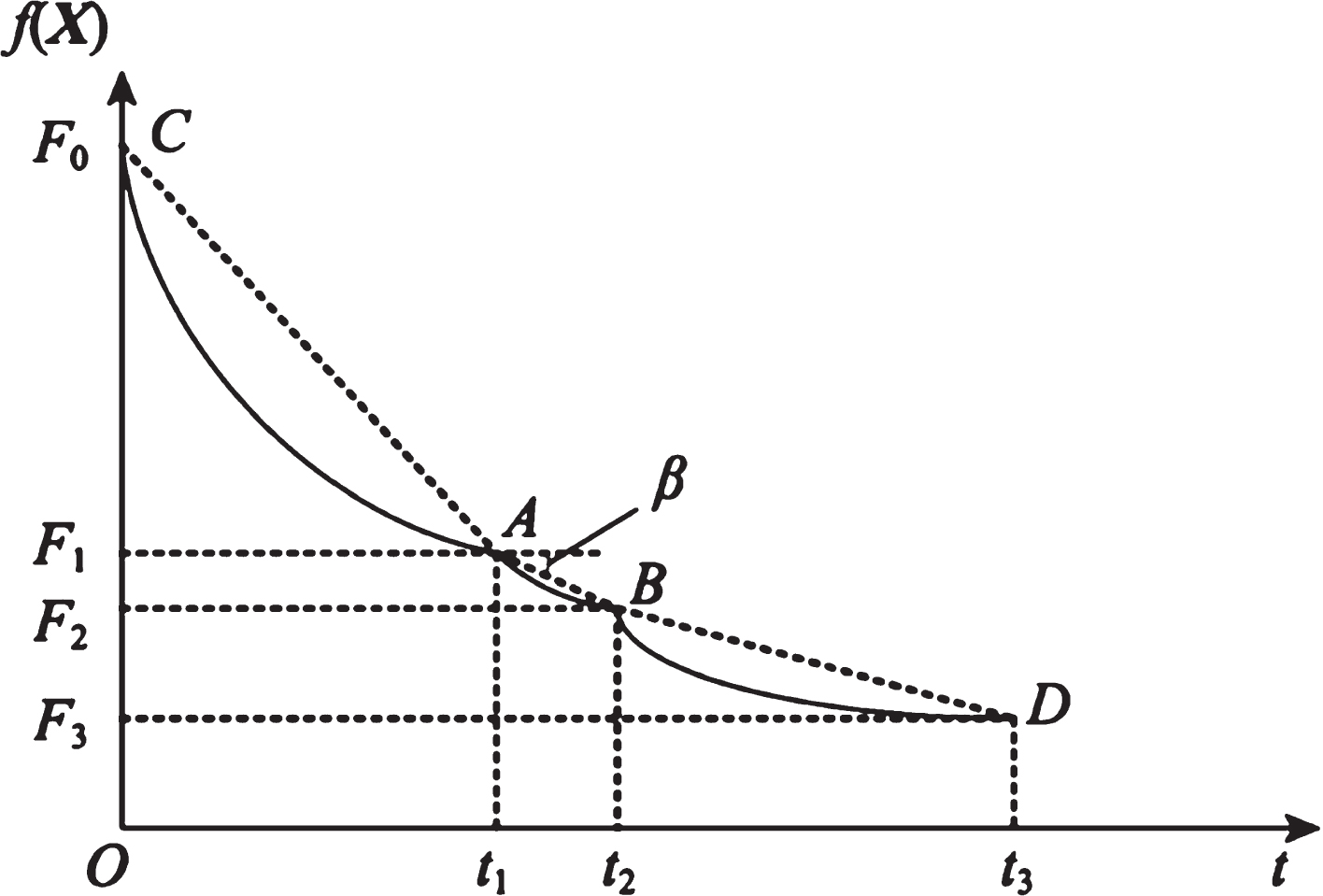The penetration and expansion ability of the population can be identified by the slope of the straight line AB, so the following formula: $slope (t_{1}) = β = \frac{180}{π} ardtan | \frac{F_{2} - F_{1}}{t_{2} - t_{1}} |$

Fig. 2

Evaluation of penetration and expansion capacity of MDO algorithm.

Obviously, if the straight line AB is steeper, the penetrating ability will be higher; if the straight line AB evolves from steep to gentle slope, the expansion ability will change from good to bad, especially when slope(t₁) is close to 0, the expansion ability becomes worse, a sticky state appears. Therefore, two thresholds λ_Ps and λ_Es must be defined to illustrate these situations: λ_Ps is used to distinguish between penetration state and expansion state, and λ_Es is used to distinguish between expansion state and sticky state.

If slope(t₁) > λ_Ps, it means that some populations stay in the penetrating state.

If λ_Es < slope(t₁)≤λ_Ps, it means that some populations are in a state of expansion.

If slope(t₁)≤λ_Es, it means that most populations have a tendency to enter a sticky state, and evolution may stop.

Now the penetration and expansion capabilities of the population are considered in the time interval [t_A, t_B]. Let CountPs(t_A,t_B) denote the number of positions in the interval [t_A, t_B], t_A≤t≤t_B that satisfies slope(t) > λ_Ps; CountEs(t_A,t_B) denote the number of positions in the interval [t_A, t_B] that satisfies λ_Es < slope_i (t)≤λ_Ps; CountSs(t_A,t_B) represents the number of positions that satisfy slope(t₁)≤λ_Es in the interval [t_A, t_B]. There are the following formulas: $CountPs (t_{A}, t_{B}) = Count (i | {slope}_{i} (t) > λ_{Ps}, t_{A} ⩽ t < t_{B})$ $\begin{matrix} CountEs (t_{A}, t_{B}) = Count (i | λ_{Es} ⩽ {slope}_{i} (t) ⩽ λ_{Ps}, \\ t_{A} ⩽ t < t_{B}) \end{matrix}$ ${CountSs (t}_{A} {, t}_{B}) = Count (i | slopei (t) < λ_{Es} {, t}_{A} ⩽ t < t_{B})$

Wherein, Count (.) is a function to calculate the position that meets the given conditions.

The measurement method of the coordination between penetration and expansion defined in the time interval [t_A, t_B] is as follows: $C_{P_{s} / E_{s}} (t_{A}, t_{B}) = \frac{1 + CountPs (t_{A}, t_{B})}{1 + CountEs (t_{A}, t_{B})}$

Wherein, C_Ps/Es(t_A,t_B) is called penetration-expansion coordination coefficient.

If C_Ps/Es(t_A,t_B) > C_Ps, it means that the search is in a penetration dominant state within the time interval [t_A,t_B].

If C_Ps/Es(t_A,t_B)≤C_Ps, it means that the search is in a state of expansion dominance within the time interval [t_A,t_B].

Similarly, the measurement method of the degree of coordination between expansion and viscosity in the time interval [t_A, t_B] can be defined as follows: $C_{E_{s} / S_{s}} (t_{A}, t_{B}) = \frac{1 + CountEs (t_{A}, t_{B})}{1 + CountSs (t_{A}, t_{B})}$

Wherein, C_Es/Ss(t_A,t_B) is called the expansion-viscosity coordination coefficient.

If C_Es/Ss(t_A,t_B) > C_Es, it means that the search is in a expansion dominant state within the time interval [t_A,t_B].

If C_Es/Ss(t_A,t_B)≤C_Es, it means that the search is in a state of viscosity dominance within the time interval [t_A,t_B].

4.2 Analysis of penetration and expansion capabilities

The Michalewicz function is chosen to illustrate the penetration and expansion capabilities of the MDO algorithm. The form of the Michalewicz function is as follows: $min E_{1} (X) = - \sum_{i = 1}^{n} \begin{matrix} sin (x_{i}) {[sin (\frac{{ix}_{i}^{2}}{π})]}^{2 m}, \\ (m = 15) \end{matrix}$

This function has the characteristics shown in Table 9. The Michalewicz function has n! local extremum points. When n = 80, there are 7.156 9×10¹¹⁸ local extremum points, so it is extremely difficult to obtain the optimal solution for this function.

Table 9
Characteristics of benchmark function F3 and Michalewicz function

Features E(X)

Multimodal? Yes

Rotated and translated? Yes, the origin (0,0,...,0) is not the global optimal objective function value

Domain of X X∈[0,10]ⁿ

Inseparable? no

The global optimal solution is known? Unknown

Does the expression contain periodic functions? Yes

The number of conditions is high? no

Extremely difficult to solve? Yes

Features	E(X)
Multimodal?	Yes
Rotated and translated?	Yes, the origin (0,0,...,0) is not the global optimal objective function value
Domain of X	X∈[0,10]ⁿ
Inseparable?	no
The global optimal solution is known?	Unknown
Does the expression contain periodic functions?	Yes
The number of conditions is high?	no
Extremely difficult to solve?	Yes

Figure 3 shows the distribution of penetration, expansion and viscous state when MDO algorithm solves the Michalewicz function in the time interval [0,694]. The calculation parameters are n = 80, E₀ = 0.005, K = 3, T = 4, τ= 3, L = 3, N = 200, G = 80000. It can be seen from Fig. 3 that when the MDO algorithm solves the Michalewicz function, CountPs(0,694) = 103, CountEs(0,694) = 297, CountSS(0,694) = 40, it takes 23.41% of the time to penetrate, 67.50% for expansion, there is only 9.09% probability of falling into a sticky state.

Fig. 3

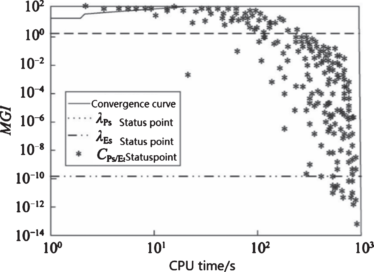
Distribution of penetration, expansion and viscosity(ɛ = 1.0E-11,λ_Ps = 1.0,λ_Es = 1.0E-10).

When the MDO algorithm solves the Michalewicz function, Fig. 4 shows the number of penetration, expansion, and viscous states in the time interval [0,694]. It can be seen from Fig. 4 that when the MDO algorithm solves the Michalewicz function, the penetration and expansion states alternate from 0 to 250 s, but the penetration state is always dominant from 0 to 250 s. Only the expansion state occurs between 250 s and 350 s; after 350 s, the expansion and the viscous state alternately appear, but the probability of the occurrence of the viscous state increases, and the expansion state always prevails after 350 s. This means that penetration and expansion are carried out sequentially from 0 to 250 s; between 250 s and 350 s, the search is close to the global optimum, and only expansion is required; when the search is carried out for 350 s, the sticky state occasionally starts to appear.

Fig. 4

Number of times of penetration, expansion and viscous state λ_Ps = 1.0,λ Es = 10^-10).

When the MDO algorithm solves the Michalewicz function, Fig. 5 shows the coordination between penetration and expansion in the time interval [0,694]. It can be seen from Fig. 5 that when the MDO algorithm solves the Michalewicz function, the penetration state is dominant from 0 to 250 s; when t = 250 s, the penetration state is dominant and reaches the maximum value; after 250 s, the penetration state is dominant. The superiority begins to decrease; on the contrary, the probability of the inflated state begins to increase. This conclusion is consistent with the conclusion obtained from Fig. 4.

Fig. 5

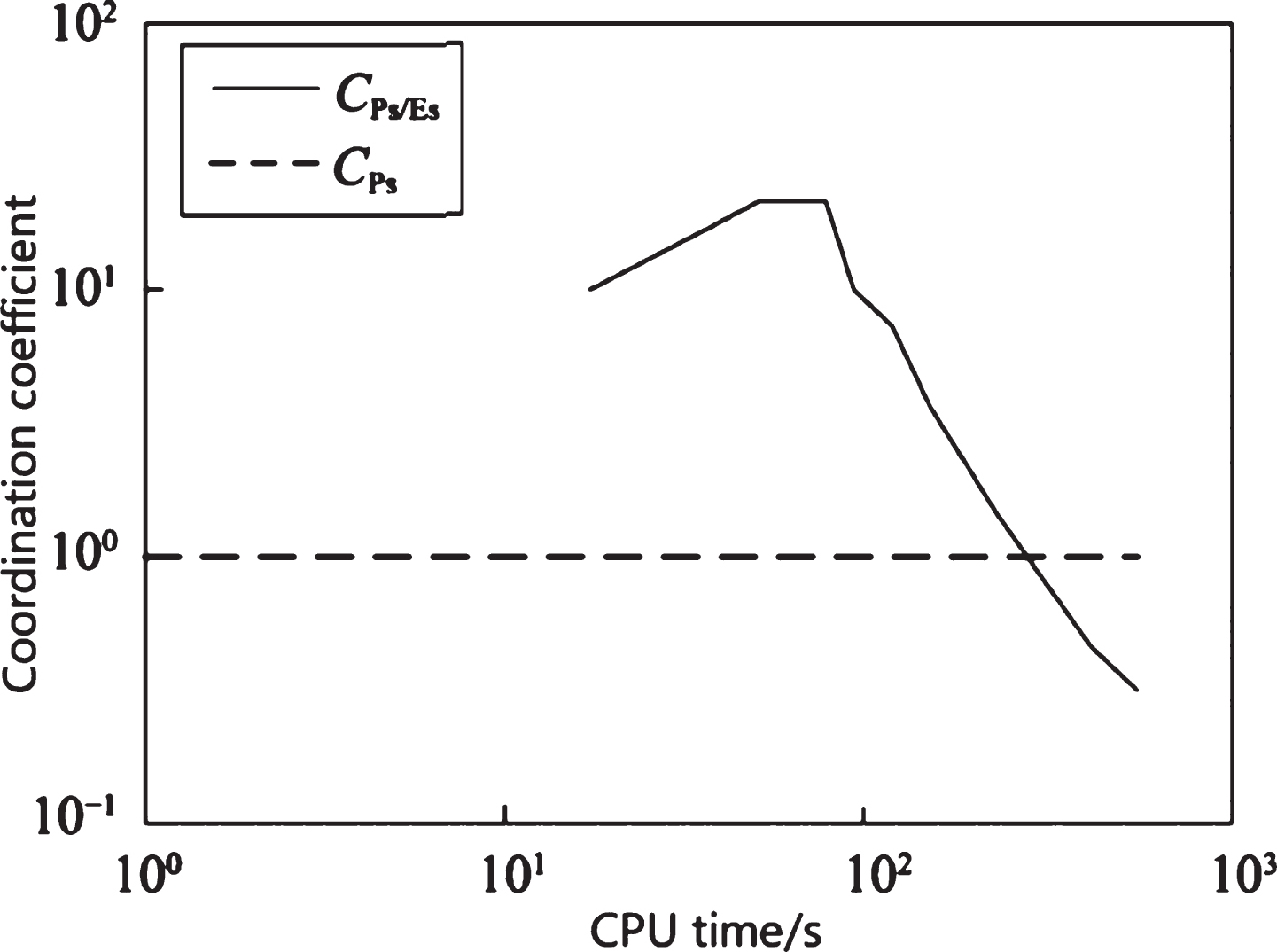
Variation of coordination coefficient of penetration and expansion with time (C_Ps = 1.0).

When the MDO algorithm solves the Michalewicz function, Fig. 6 shows the coordination between expansion and stickiness in the time interval [0,694]. It can be seen from Fig. 6 that when the MDO algorithm solves the Michalewicz function, when t = 350 s, the expansion state dominance reaches the maximum value, and then the number of occurrences of the dominance state begins to decrease. On the contrary, the number of occurrences of the sticky state begins to increase, but the number of occurrences of the sticky state is always not dominant.

Fig. 6

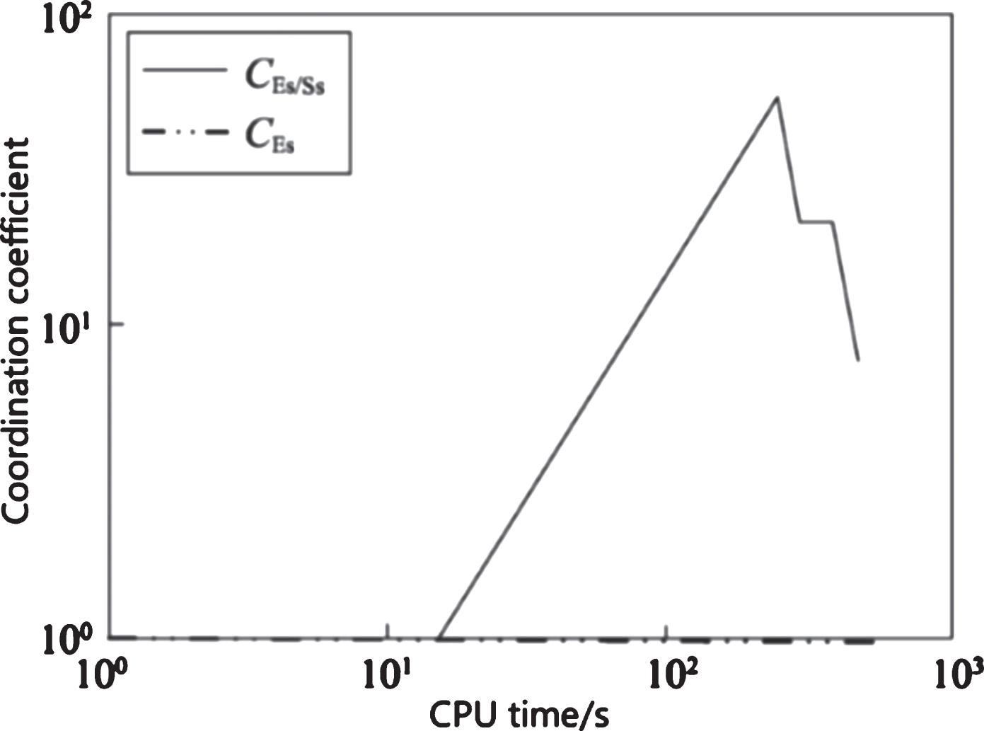
Variation of coordination coefficient of expansion and viscosity with time (C_Es = 1.0).

From the above analysis, it can be seen that when solving optimization problems with a large number of local optimal solutions and optimization problems with high condition numbers, the MDO algorithm shows a good global optimization ability, and the balance between the local optimization ability and the global optimization ability is well control.

5 Conclusion

In this paper, a new optimization algorithm with global convergence is proposed based on the kinetic theory of microbial cultivation in the hybrid food chain with time delay. Compared with other typical swarm intelligence algorithms, the MDO algorithm has the following characteristics:

Absorption operators, grabbing operators, hybrid operators and poison operators can increase its search ability.

The random method is used to determine the relevant parameters in each operator, which not only greatly reduces the number of parameter inputs, but also enables the model to better express the actual situation.

The microbial culture process involved in the algorithm fully reflects the concentration of various microbial populations, the amount of culture solution and its nutrient concentration, the concentration of toxic substances contained in the regular amount of culture solution, the period of culture solution, and the direction of culture solution. Complex changes in parameters such as the lag time of microbial transformation.

All operators are constructed by using the kinetic theory of hybrid food chain microbial pulse culture with time lag and the interaction relationship between microbial populations, and it do not need to be related to the optimization problem to be solved. Therefore, the MDO algorithm has good universality.

The impulse increase in the concentration of the culture medium and the toxic substances contained in it will cause the trial solution to suddenly shift from one state to another. This property helps to make the search jump out of the local optimal trap.

The algorithm takes into account the discontinuous intervention of external factors in the process of microbial population cultivation.

The interaction between the microbial populations involved in the algorithm is rich and colorful, reflecting the complex predation-being relationship and competition relationship among the microbial populations in the culture system.

The algorithm reflects the complex changes of various parameters in the microbial culture dynamics model.

When performing iterative calculations, the algorithm only processes 1/1 000∼1/100 of the number of features of each population each time, which greatly reduces the time complexity. Therefore, the MDO algorithm is suitable for solving high-dimensional optimization problems.

The next steps to improve the MDO algorithm are as follows:

The microbial culture kinetic model is used to optimize the relevant parameters of the MDO algorithm to make these parameter settings more reasonable.

In-depth study of the dynamic characteristics of absorption operators, grabbing operators, hybrid operators and toxin operators.

In-depth study of the dynamic characteristics of microbial populations.

Footnotes

Acknowledgments

This work was supported by the Scientific Research Project (No: 20B335, No: 18C1122) of Hunan Provincial Education Department, China & Hunan Natural Science Foundation (Grant No: 2019JJ40154), Hunan Province, China (Grant No. 2019JJ40154).

References

Dahi

Z.L.

, Mezioud

and Draa

, A quantum-inspired genetic algorithm for solving the antenna positioning problem, Swarm and Evolutionary Computation 31(1) (2016), 24–63.

, Shi

R.Z

, et al., Real-Time Patient-Specific ECG Arrhythmia Detection by Quantum Genetic Algorithm of Least Squares Twin SVM, Journal of Beijing Institute of Technology 29(1) (2020), 29–37. doi: 10.15918/j.jbit1004-0579.18156

Zhao

J.S.

, Gu

Y.T.

and Feng

Z.G.

, Optimization of Processing Parameters of Power Spinning for Bushing Based on Neural Network and Genetic Algorithms, Journal of Beijing Institute of Technology 28(3) (2019), 606–616. doi: 10.15918/j.jbit1004-0579.18063

Wang

Z.Z.

, Li

H.Y.

, Han

, et al., Arrhythmia Classification Based on Multiple Features Fusion and Random Forest Using ECG, Journal of Medical Imaging & Health Informatics 9(8) (2019), 1645–1654.

Feeny

A.K.

, Chung

M.K.

, et al., Artificial Intelligence and Machine Learning in Arrhythmias and Cardiac Electrophysiology, Circulation: Arrhythmia and Electrophysiology 13(8) (2020), Doi: 10.1161/CIRCEP.119.007952

Lin

P.P.

, Zhang

and Contreras

M.A.

, Automatically configuring ACO using multilevel ParamILS to solve transportation planning problems with underlying weighted networks, Swarm and Evolutionary Computation 20(1) (2015), 48–57.

Wang

H.M.

, Li

J.Z.

, et al., Multi-objective test case prioritization based on multi-population cooperative particle swarm optimization, The Journal of China Universities of Posts and Telecommunications 27(1) (2020), 38–50. doi: 10.19682/j.cnki.1005-8885.2020.0003

, Zhang

E.Z.

and Chen

Q.W.

, Rotary unmanned aerial vehicles path planning in rough terrain based on multi-objective particle swarm optimization, Journal of Systems Engineering and Electronics 31(1) (2020), 130–141. doi: 10.21629/JSEE.2020.01.14

Wang

Y.K.

and Chen

X.V.

, Hybrid quantum particle swarm optimization algorithm and its application, Science China Information Sciences 63(5) (2020), 199–201.

10.

Fei

, Liu

and Hu

, Research on swarm intelligence optimization algorithm, The Journal of China Universities of Posts and Telecommunications 27(3) (2020), 1–20. doi: 10.19682/j.cnki.1005–8885.2020.0012

11.

Zhang

D.Q.

and Jiang

M.Y.

, Parallel discrete lion swarm optimization algorithm for solving traveling salesman problem, Journal of Systems Engineering and Electronics 31(4) (2020), 751–760. doi: 10.23919/JSEE.2020.000050

12.

Wolpert

D.H.

and Macready

W.G.

, No free lunch theorems for optimization, IEEE Transactions on Evolutionary Computation 1(1) (1997), 67–82.

13.

Huang

G.Q.

, Function optimization algorithm based on SIRQV epidemic dynamic model, Journal of Computation Science 8(1) (2015), 62–92.

14.

Chen

L.S.

, Meng

X.Z.

and Jiao

J.J.

, Biodynamics. Beijing: Science Press, (2009).

15.

Huang

G.Q.

, Zhao

W.J.

and Lu

Q.Q.

, Population dynamics optimization based on 3 populations Lotka-Volterra model, Computer Science 40(8) (2013), 214–219.

16.

Huang

G.Q.

, Li

and Lu

Q.Q.

, Population dynamics-based optimization, Computer Science 40(11) (2013), 280–286.

17.

Q.Q.

and Huang

G.Q.

, Method of determining the optimal guidance path of elimination in-site concentrated gushed out mineral dust resulting from many initiating places in an underground mine, Industrial Minerals & Processing 47(3) (2018), 37–42.

18.

Q.Q.

and Huang

G.Q.

, Optimum positioning method for mineral dust collecting stations in multi-stage hybrid local ventilation subsystems, Industrial Minerals & Processing 47(2) (2018), 46–51.

19.

Pantoja

, Obando

and Quijano

, Distributed optimization with information-constrained population dynamics, Journal of the Franklin Institute 356(1) (2019), 209–236.

20.

Heidari

A.A.

, Hammouri

A.I.

, et al., Evolutionary Population Dynamics and Grasshopper Optimization approaches for feature selection problems, Knowledge-Based Systems 145(Apr.1) (2018), 25–45.

21.

Meng

Z.Y.

, Pan

J.S.

and Zheng

W.M.

, Differential evolution utilizing a handful top superior individuals with bionic bi-population structure for the enhancement of optimization performance, Enterprise Information Systems 14(2) (2020), 221–242.

22.

Huang

G.Q.

, SIS epidemic model- based optimization, Journal of Computational Science 5(1) (2014), 32–50.

23.

Liang

J.J.

, Qu

B.Y.

, Suganthan

P.N.

, et al., Problem definitions and evaluation criteria for the CEC 2013 special session on real-parameter optimization. Singapore: Nanyang Technological University 2012-12 [2013-10-20]. http://www.ntu.edu.sg/home/epnsugan/index_files/cec-2013/Definitions of CEC 13 benchmark suite 0117.pdf.

24.

Chuang

Y.C.

, Chen

C.T.

and Hwang

, A simple and efficient real-coded genetic algorithm for constrained optimization, Applied Soft Computing 38(1) (2016), 87–105.

25.

Korosec

, Silc

and Filipic

, The differential ant-stigmergy algorithm, Information Sciences 192(1) (2012), 82–97.

26.

Beheshti

and Shamsuddin

S.M.

, Non-parametric particle swarm optimization for global optimization, Applied Soft Computing 28(1) (2015), 345–359.

27.

Al-Roomi

A.R.

and El-Hawary

M.E.

, Metropolis biogeographybased optimization, Information Sciences 360(1) (2016), 73–95.

28.

Souza

S.S.F.

, Romero

, Pereira

, et al., Artificial immune algorithm applied to distribution system reconfiguration with variable demand, Electrical Power and Energy Systems 82(1) (2016), 561–568.

29.

Zhao

Z.W.

, Yang

J.M.

, Hu

Z.Y.

, et al., A differential evolution algorithm with self-adaptive strategy and control parameters based on symmetric Latin hypercube design for unconstrained optimization problems, European Journal of Operational Research 250(1) (2016), 30–45.

30.

Mernik

, Liu

S.H.

, Karaboga

, et al., On clarifying misconceptions when comparing variants of the artificial bee colony algorithm by offering a new implementation, Information Sciences 291(1) (2015), 115–127.

31.

Crepinsek

, Liu

S.H.

and Mernik

, Replication and comparison of computational experiments in applied evolutionary computing: common pitfalls and guidelines to avoid them, Applied Soft Computing 19(1) (2014), 161–170.

32.

Derrac

, Garcia

, Molina

, et al., A practical tutorial on the use of nonparametric statistical tests as a methodology for comparing evolutionary and swarm intelligence algorithms, Swarm and Evolutionary Computation 1(1) (2011), 3–18.