υ -Nonparallel parametric margin fuzzy support vector machine

Abstract

Classification problem is an important research direction in machine learning. υ-nonparallel support vector machine (υ-NPSVM) is an important classifier used to solve classification problems. It is widely used because of its structural risk minimization principle, kernel trick, and sparsity. However, when solving classification problems, υ-NPSVM will encounter the problem of sample noises and heteroscedastic noise structure, which will affect its performance. In this paper, two improvements are made on the υ-NPSVM model, and a υ-nonparallel parametric margin fuzzy support vector machine (par-υ-FNPSVM) is established. On the one hand, for the noises that may exist in the data set, the neighbor information is used to add fuzzy membership to the samples, so that the contribution of each sample to the classification is treated differently. On the other hand, in order to reduce the effect of heteroscedastic structure, an insensitive loss function is introduced. The advantages of the new model are verified through UCI machine learning standard data set experiments. Finally, Friedman test and Bonferroni-Dunn test are used to verify the statistical significance of it.

Keywords

Classification problem sample noises heteroscedastic noise structure parameter margin nearest neighbor fuzzy membership

1 Introduction

Machine learning is a common research hotspot in the field of artificial intelligence and pattern recognition. Support Vector Machine (SVM) is a new technology introduced by Vapnik et al. in the 1990 s to address machine learning problems with optimization methods [1 –5], and have been successfully applied in a wide variety of fields such as face recognition, text categorization, bioinformatics [6 –12], etc.

Recently, a branch of SVM, nonparallel hyperplane SVM which considers the difference in data distribution of samples, is developed and has attracted many interests. The representative algorithms include the generalized eigenvalue proximal support vector machine (GEPSVM) [13 –15], the twin support vector machine (TWSVM) [16 –18] and the nonparallel support vector machine (NPSVM) [19, 20]. For the GEPSVM, it opened a new chapter in the research of non-parallel hyperplane SVM classification methods. In this method, the samples of each class are located near one hyperplane and maintain a clear separation from the other. Two non-parallel planes are represented by eigenvectors, which depend on the smallest eigenvalue obtained from the generalized eigenvalue problem. For TWSVM, it seeks two non-parallel proximal hyperplanes such that each hyperplane is close to one of the two classes and is at least one distance from the other. The formulation of TWSVM is totally different from that of GEPSVM and is very much in line with standard SVM. It is implemented by solving two smaller QPPs instead of a larger one, which increases the TWSVM training speed by approximately fourfold compared to that of standard SVM. Twin support vector machines (TWSVM) have been studied extensively [21 –25]. For NPSVM, it seeks two nonparallel hyperplanes, such that each class locates as much as possible in the ɛ-band of the hyperplane and each hyperplane is at least one distance from the other. NPSVM has many advantages over TWSVM in theory such as the same two convex quadratic programming problems for both linear and nonlinear cases, no need to compute the inverse matrices before training and sparsity. Therefore, NPSVM has attracted a lot of attention [26 –28].

In NPSVM, the parameter ɛ and the regularization constant C controlling the sparseness need to be specified beforehand. The value of them is qualitatively clear: the larger C implies the more attention has been paid to minimizing the training error, the larger ɛ implies greater sparsity. However, it is gravely lacking in quantitative meaning, which means that we cannot estimate the sparseness even we are given the value of C and ɛ. In order to overcome this problem, υ-NPSVM [29 –31] is introduced. Parameter υ lets one effectively control the number of support vectors.

However, when solving classification problems, υ-NPSVM will encounter the problem of sample noises and heteroscedastic noise structure, which will affect its performance. In υ-NPSVM, it is assumed that the noise level is uniform throughout the domain. However, in many practical problems, there may be noises in the data samples and they may not be uniform which is called heterogeneous noises. That means some noises depend largely on the position of the sample points. In response to these problems, a parameter-insensitive loss function and a nearest neighbor fuzzy membership are introduced respectively in υ-NPSVM. Combining the above two improvements, this paper constructs a υ-nonparallel parametric margin fuzzy support vector machine model (par-υ-FNPSVM). Based on the data of heteroscedasticity structure, contribution of each sample to the classification is treated differently. So the classification accuracy and generalization ability is improved obviously. Thereafter, two statistical test methods also help us to verify the statistical significance of the established model.

The rest of this paper is organized as follows. Section 2 is a review of υ-NPSVM. In section 3, parameter margin fuzzy υ-nonparallel support vector machine is presented in detail. Experimental results and discussions are given in section 4. The last section is the conclusion.

2 υ-Nonparallel Support Vector Machine (υ-NPSVM)

2.1 Linear υ-NPSVM

In this section, a review of linear and nonlinear υ-NPSVM will be described briefly.

Consider the training set T = { (x₁, + 1) , . . . , (x_p, + 1) , (x_p+1, - 1) , . . . , (x_p+q, - 1), where x_i ∈ Rⁿ, i = 1, …, p + q the inputs are, y_i∈ { - 1, 1 } are the outputs. υ-NPSVM is to find two nonparallel hyperplanes $(w_{+} \cdot x) + b_{+} = 0 and (w_{-} \cdot x) + b_{-} = 0$ (1) by solving the following two QPPs. $\begin{matrix} min_{w_{+}, b_{+}, η_{+}^{(*)}, ξ_{-}} \frac{1}{2} {∥ w_{+} ∥}^{2} + C_{1} (v_{1} ɛ_{+} + \frac{1}{p} \sum_{i = 1}^{p} (η_{i} + η_{i}^{*})) \\ + (- v_{2} ρ_{+} + \frac{1}{q} \sum_{j = p + 1}^{p + q} ξ_{j}) \\ s . t . (w_{+} \cdot x_{i}) + b_{+} ⩽ ɛ_{+} + η_{i}, i = 1, \dots, p \\ - (w_{+} \cdot x_{i}) - b_{+} ⩽ ɛ_{+} + η_{i}^{*}, i = 1, \dots, p \\ (w_{+} \cdot x_{j}) + b_{+} ⩽ - ρ_{+} + ξ_{j}, j = p + 1, \dots, p + q \end{matrix}$ (2) $\begin{matrix} η_{i}, η_{i}^{*} ⩾ 0, i = 1, \dots, p \\ ξ_{j} ⩾ 0, j = p + 1, \dots, p + q \\ ρ_{+} ⩾ 0, ɛ_{+} ⩾ 0 \end{matrix}$ and $\begin{matrix} min_{w_{-}, b_{-}, η_{-}^{(*)}, ξ_{+}} \frac{1}{2} {∥ w_{-} ∥}^{2} + C_{2} (v_{3} ɛ_{-} + \frac{1}{q} \sum_{i = p + 1}^{p + q} (η_{i} + η_{i}^{*})) \\ + (- v_{4} ρ_{-} + \frac{1}{p} \sum_{j = 1}^{p} ξ_{j}) \\ s . t . (w_{-} \cdot x_{i}) + b_{-} ⩽ ɛ_{-} + η_{i}, i = p + 1, \dots, p + q \\ - (w_{-} \cdot x_{i}) - b_{-} ⩽ ɛ_{-} + η_{i}^{*}, i = p + 1, \dots, p + q \\ (w_{-} \cdot x_{j}) + b_{-} ⩽ ρ_{-} - ξ_{j}, j = 1, \dots, p \\ η_{i}, η_{i}^{*} ⩾ 0, i = p + 1, \dots, p + q \\ ξ_{j} ⩾ 0, j = 1, \dots, p \\ ρ_{-} ⩾ 0, ɛ_{-} ⩾ 0 \end{matrix}$ (3)

Among them, C_i ⩾ 0, i = 1, 2 are penalty parameters, which control the coordination between the maximum boundary and the number of misclassifications. Parameters v_i ∈ (0, 1] , i = 1, …, 4 control the sparsity of positive and negative classes respectively. $ξ_{+} = {(ξ_{1}, \dots, ξ_{p})}^{T}, ξ_{-} = (ξ_{p + 1}, \dots, ξ_{p + q})^{T}, η_{+}^{(*)} = (η_{+}^{T}, η_{+}^{* T})^{T}$ $= (η_{1}, \dots, η_{P}, η_{1}^{*}, \dots, η_{p}^{*})^{T}$ , $η_{-}^{(*)} = (η_{-}^{T}, η_{-}^{* T})^{T} = (η_{p + 1}, \dots$ , $η_{P + q}, η_{p + 1}^{*}, \dots, η_{p + q}^{*})^{T}$ are slack variables. $\sum_{i = 1}^{p} (η_{i} + η_{i}^{*})$ is empirical risk and it requires the positive sample points to be in the ɛ-band of the positive hyperplane (w₊ · x) + b₊ = ɛ and (w_- · x) + b_- = ɛ as much as possible. $\sum_{j = p + 1}^{p + q} ξ_{j}$ is another empirical risk and it limits the negative sample point to be located below the plane (w₊ · x) + b₊ = - ρ₊. The geometric interpretation of υ-NPSVM is shown in Fig. 1.

Fig. 1

Geometrical illustration of υ-NPSVM in R².

The Wolfe dual forms of the original problems (2) and (3) are: $\begin{matrix} min_{α, β, γ} \frac{1}{2} \sum_{i = 1}^{p} \sum_{j = 1}^{p} α_{i} α_{j} x_{i} \cdot x_{j} + \frac{1}{2} \sum_{i = 1}^{p} \sum_{j = 1}^{p} β_{i} β_{j} x_{i} \cdot x_{j} \\ + \frac{1}{2} \sum_{i = p + 1}^{p + q} \sum_{j = p + 1}^{p + q} γ_{i} γ_{j} x_{i} \cdot x_{j} + \sum_{i = 1}^{p} \sum_{j = p + 1}^{p + q} α_{i} γ_{j} x_{i} \cdot x_{j} \\ - \sum_{i = 1}^{p} \sum_{j = p + 1}^{p + q} β_{i} γ_{j} x_{i} \cdot x_{j} - \sum_{i = 1}^{p} \sum_{j = 1}^{p} α_{i} γ_{j} x_{i} \cdot x_{j} \end{matrix}$ $\begin{matrix} s . t . \sum_{i = 1}^{p} β_{i} = \sum_{i = 1}^{p} α_{i} + \sum_{j = p + 1}^{p + q} γ_{j} \\ - v_{2} + \sum_{j = p + 1}^{p + q} γ_{j} ⩾ 0 \\ C_{1} v_{1} - \sum_{i = 1}^{p} α_{i} - \sum_{i = 1}^{p} β_{i} ⩾ 0 \\ 0 ⩽ α ⩽ \frac{C_{1}}{p} e_{+} \\ 0 ⩽ β ⩽ \frac{C_{1}}{p} e_{+} \\ 0 ⩽ γ ⩽ \frac{1}{q} e_{-} \end{matrix}$ (4) and $\begin{matrix} min_{α, β, γ} \frac{1}{2} \sum_{i = 1}^{p} \sum_{j = 1}^{p} γ_{i} γ_{j} x_{i} \cdot x_{j} + \frac{1}{2} \sum_{i = p + 1}^{p + q} \sum_{j = p + 1}^{p + q} β_{i} β_{j} x_{i} \cdot x_{j} \\ + \frac{1}{2} \sum_{i = p + 1}^{p + q} \sum_{j = p + 1}^{p + q} α_{i} α_{j} x_{i} \cdot x_{j} + \sum_{i = p + 1}^{p + q} \sum_{j = 1}^{p} α_{i} β_{j} x_{i} \cdot x_{j} \\ - \sum_{i = p + 1}^{p + q} \sum_{j = 1}^{p} β_{i} γ_{j} x_{i} \cdot x_{j} - \sum_{i = 1 + p}^{p + q} \sum_{j = 1}^{p} α_{i} γ_{j} x_{i} \cdot x_{j} \end{matrix}$ (5) $\begin{matrix} min_{α, β, γ} \frac{1}{2} \sum_{i = 1}^{p} \sum_{j = 1}^{p} γ_{i} γ_{j} x_{i} \cdot x_{j} + \frac{1}{2} \sum_{i = p + 1}^{p + q} \sum_{j = p + 1}^{p + q} β_{i} β_{j} x_{i} \cdot x_{j} \\ + \frac{1}{2} \sum_{i = p + 1}^{p + q} \sum_{j = p + 1}^{p + q} α_{i} α_{j} x_{i} \cdot x_{j} + \sum_{i = p + 1}^{p + q} \sum_{j = 1}^{p} α_{i} β_{j} x_{i} \cdot x_{j} \\ - \sum_{i = p + 1}^{p + q} \sum_{j = 1}^{p} β_{i} γ_{j} x_{i} \cdot x_{j} - \sum_{i = 1 + p}^{p + q} \sum_{j = 1}^{p} α_{i} γ_{j} x_{i} \cdot x_{j} \\ s . t . \sum_{i = 1}^{p} α_{i} = \sum_{i = 1}^{p} β_{i} + \sum_{j = p + 1}^{p + q} γ_{j} \\ - v_{4} + \sum_{j = 1}^{p} γ_{j} ⩾ 0 \\ C_{2} v_{3} - \sum_{i = p + 1}^{p + q} α_{i} - \sum_{i = p + 1}^{p + q} β_{i} ⩾ 0 \end{matrix}$ $\begin{matrix} 0 ⩽ α ⩽ \frac{C_{2}}{q} e_{-} \\ 0 ⩽ β ⩽ \frac{C_{2}}{p} e_{-} \\ 0 ⩽ γ ⩽ \frac{1}{p} e_{+} \end{matrix}$ where in (4), α = (α₁, …, α_p) ^T, β = (β₁, …, β_p) ^T, γ = (γ₁, …, γ_p) ^T, $θ^{(i)} = (θ_{1}^{(i)}, \dots, θ_{p}^{(i)})^{T}, i = 1, 2,$ $θ^{(3)} = (θ_{p + 1}^{(3)}, \dots, θ_{p + q}^{(3)})^{T}$ are Lagrange multipliers.

Similarly, in (5), α = (α_p+1, …, α_p+q) ^T, β = (β_p+1, …, β_p+q) ^T $γ = {(γ_{1}, \dots, γ_{q})}^{T}, θ^{(i)} = (θ_{p + 1}^{(i)}, {\dots, θ_{p + q}^{(i)})}^{T}$ , i = 1, 2, $θ^{(3)} = {(θ_{1}^{(3)}, \dots, θ_{p}^{(3)})}^{T}, θ^{(4)} \in R^{+}, θ^{(5)} \in R^{+}$ are Lagrange multipliers.

By calculating the dual problems (4), the solution (α, β, γ) is obtained, w₊ can be expressed as $w_{+} = \sum_{i = 1}^{p} (β_{i} - α_{i}) x_{i} + \sum_{j = p + 1}^{p + q} γ_{j} x_{j}$ (6) and choose a component of $α_{i} \in (0, \frac{C_{1}}{p})$ , then $b_{+} = - \frac{1}{2} ((w_{+} \cdot x_{i}) + (w_{+} \cdot x_{j})) .$ (7)

Similarly, by calculating the dual problem (5), w _ can be expressed as $w_{-} = \sum_{i = p + 1}^{p + q} (β_{i} - α_{i}) x_{i} + \sum_{j = 1}^{p} γ_{j} x_{j},$ (8) and choose a component of $α_{i} \in (0, \frac{C_{2}}{q})$ , then $b_{-} = \frac{1}{2} ((w_{-} \cdot x_{i}) + (w_{-} \cdot x_{j})),$ (9)

Then, the two decision functions are obtained $f_{+} (x) = \sum_{i = 1}^{p} (β_{i} - α_{i}) (x_{i} \cdot x) - \sum_{j = p + 1}^{p + q} γ_{j} (x_{j} \cdot x) + b_{+}$ (10) and $f_{-} (x) = \sum_{i = p + 1}^{p + q} (β_{i} - α_{i}) (x_{i} \cdot x) + \sum_{j = 1}^{p} γ_{j} (x_{j} \cdot x) + b_{-}$ (11)

2.2 Nonlinear υ-NPSVM

In many cases, the sample points cannot be separated by the linear class boundary. Therefore, we can use the kernel technique to extend the linear υ-NPSVM to the nonlinear case. After the sample points are projected into the high-dimensional feature space, they are easier to separate. By introducing the kernel function K (x_i, x_j) = φ (x_i) · φ (x_j), the optimization problems corresponding to problems (4) and (5) are as follows:

$\begin{matrix} min_{α, β, γ} \frac{1}{2} \sum_{i = 1}^{p} \sum_{j = 1}^{p} α_{i} α_{j} K (x_{i}, x_{j}) + \frac{1}{2} \sum_{i = 1}^{p} \sum_{j = 1}^{p} β_{i} β_{j} K (x_{i}, x_{j}) \\ + \frac{1}{2} \sum_{i = p + 1}^{p + q} \sum_{j = p + 1}^{p + q} γ_{i} γ_{j} K (x_{i}, x_{j}) + \sum_{i = 1}^{p} \sum_{j = p + 1}^{p + q} α_{i} γ_{j} K (x_{i}, x_{j}) \\ - \sum_{i = 1}^{p} \sum_{j = p + 1}^{p + q} β_{i} γ_{j} K (x_{i}, x_{j}) - \sum_{i = 1}^{p} \sum_{j = 1}^{p} α_{i} γ_{j} K (x_{i}, x_{j}) \\ s . t . \sum_{i = 1}^{p} β_{i} = \sum_{i = 1}^{p} α_{i} + \sum_{j = p + 1}^{p + q} γ_{j} \\ - v_{2} + \sum_{j = p + 1}^{p + q} γ_{j} ⩾ 0 \\ C_{1} v_{1} - \sum_{i = 1}^{p} α_{i} - \sum_{i = 1}^{p} β_{i} ⩾ 0 \end{matrix}$ (12)

$\begin{matrix} 0 ⩽ α ⩽ \frac{C_{1}}{p} e_{+} \\ 0 ⩽ β ⩽ \frac{C_{1}}{p} e_{+} \\ 0 ⩽ γ ⩽ \frac{1}{q} e_{-} \end{matrix}$ and

$\begin{matrix} min_{α, β, γ} \frac{1}{2} \sum_{i = 1}^{p} \sum_{j = 1}^{p} γ_{i} γ_{j} K (x_{i} \cdot x_{j}) + \frac{1}{2} \sum_{i = p + 1}^{p + q} \sum_{j = p + 1}^{p + q} β_{i} β_{j} K (x_{i} \cdot x_{j}) \\ + \frac{1}{2} \sum_{i = p + 1}^{p + q} \sum_{j = p + 1}^{p + q} α_{i} α_{j} K (x_{i} \cdot x_{j}) + \sum_{i = p + 1}^{p + q} \sum_{j = 1}^{p} α_{i} β_{j} K (x_{i} \cdot x_{j}) \\ - \sum_{i = p + 1}^{p + q} \sum_{j = 1}^{p} β_{i} γ_{j} K (x_{i} \cdot x_{j}) - \sum_{i = 1 + p}^{p + q} \sum_{j = 1}^{p} α_{i} γ_{j} K (x_{i} \cdot x_{j}) \end{matrix}$ $\begin{matrix} s . t . \sum_{i = 1}^{p} α_{i} = \sum_{i = 1}^{p} β_{i} + \sum_{j = p + 1}^{p + q} γ_{j} \\ - v_{4} + \sum_{j = 1}^{p} γ_{j} ⩾ 0 \\ C_{2} v_{3} - \sum_{i = p + 1}^{p + q} α_{i} - \sum_{i = p + 1}^{p + q} β_{i} ⩾ 0 \\ 0 ⩽ α ⩽ \frac{C_{2}}{q} e_{-} \\ 0 ⩽ β ⩽ \frac{C_{2}}{p} e_{-} \\ 0 ⩽ γ ⩽ \frac{1}{p} e_{+} \end{matrix}$ (13)

By solving two convex QPPs (12) and (13), we get the solution (α, β, γ), and two decision functions are obtained.

$f_{+} (x) = \sum_{i = 1}^{p} (β_{i} - α_{i}) K (x_{i}, x) - \sum_{j = p + 1}^{p + q} γ_{j} K (x_{j}, x) + b_{+}$ (14)

and

$f_{-} (x) = \sum_{i = p + 1}^{p + q} (β_{i} - α_{i}) K (x_{i}, x) + \sum_{j = 1}^{p} γ_{j} K (x_{j}, x) + b_{-}$ (15)

3 υ-Nonparallel Parametric Margin Fuzzy Support Vector Machine (par-υ-FNPSVM)

In order to solve the problem of heteroscedastic noise encountered in classification problems and the influence of noises in training, a parameter margin function and a fuzzy membership degree are introduced on the basis of υ-NPSVM, thereby constructing the par-υ-FNPSVM model. The introduction of parameter margin function is to solve the problem of heteroscedastic noise. Introducing the nearest neighbor chain fuzzy membership is to reduce the influence of noises on finding the best hyperplanes. The detailed flow chart of this method is shown in Fig. 2.

Fig. 2

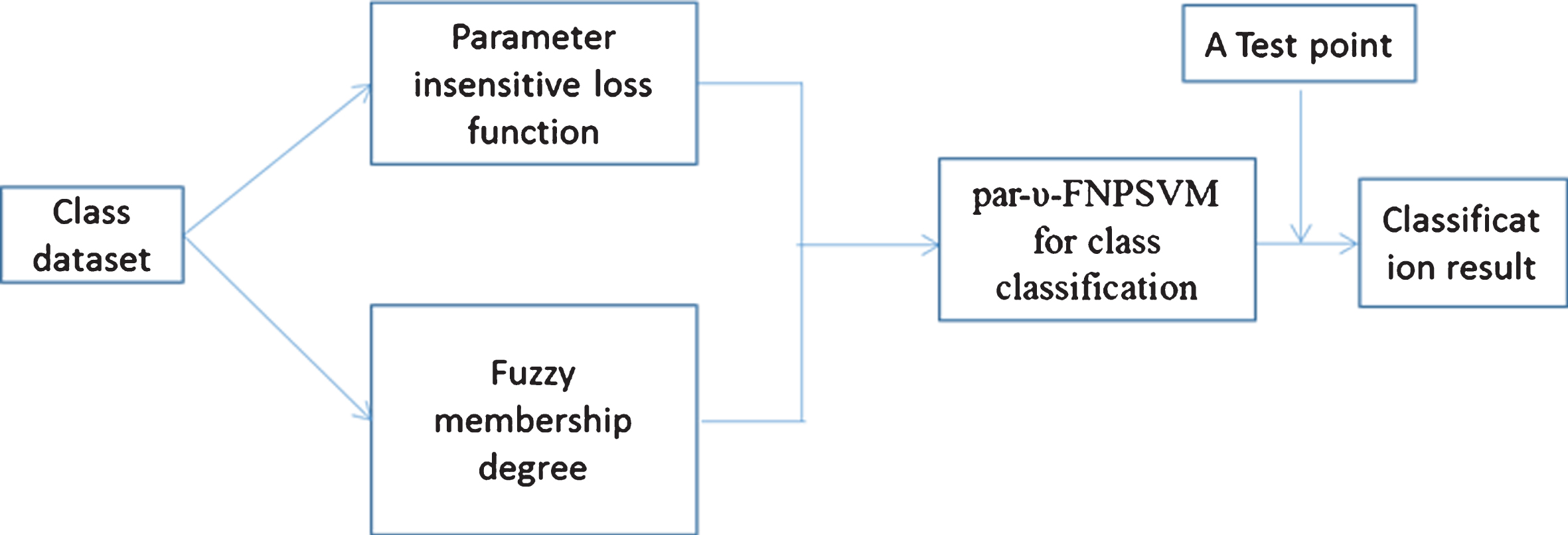
Flow chart of par-υ-FNPSVM.

3.1 The preparatory work

3.1.1 Define parameter margin loss function

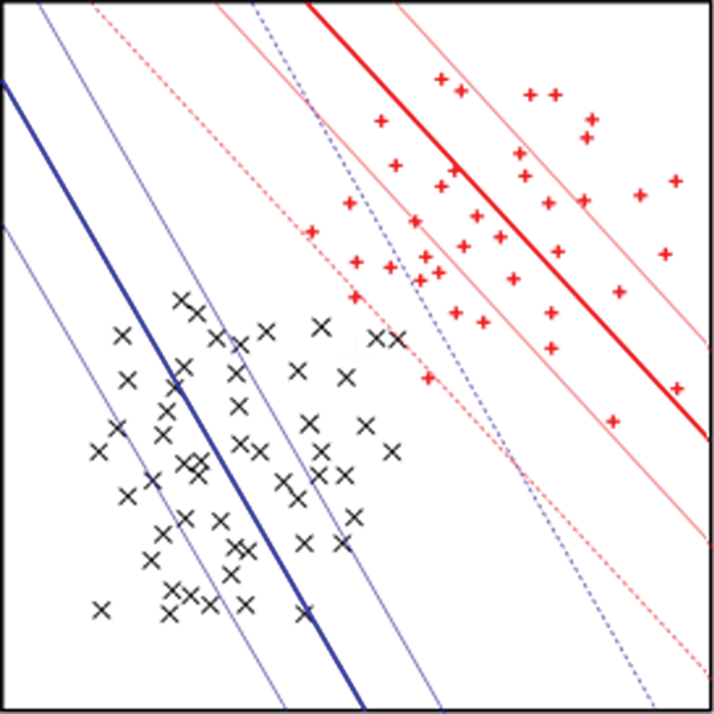
We know that υ-NPSVM assumes the noise level is uniform throughout the domain, but in fact this assumption is usually not true. There may be heteroscedasticity noise in the sample points. In this paper, in the υ-NPSVM model, improvement is made by adding a parameter margin loss function. The parameter margin loss function L^g (x, y, f) is defined as $\begin{matrix} L^{g} (x, y, f) = | y - f (x) |_{g} \\ = {\begin{matrix} 0 & if | y - f (x) | ⩽ g (x) \\ | y - f (x) | - g (x) & other \end{matrix} \end{matrix}$ (16) where f (x) and g (x) are real-valued functions on the domain Rⁿ, x ∈ Rⁿ, f (x) = w · x + b is the decision function, g (x) = u · x + d is the parameter margin function, x∈ Rⁿ, y ∈ { - 1, 1 }.

In other words, we do not care about errors as long as they are inside the parametric-margin zone f (x) ± g (x). Only the points outside the parametric-margin zone contribute to the cost, insofar as the deviations are penalized in a linear fashion. The goal of adding L^g (x, y, f) to υ-NPSVM is to automatically adjust the parameter margin area of arbitrary shape and minimum size to include the data model. By replacing ρ in the υ-NPSVM model with a parameter margin function g (x) = u · x + d, it can improve the problem of poor classification accuracy caused by heteroscedastic noise. Figure 3 depicts the situation graphically.

Fig. 3

υ-NPSVM algorithm with parametric margin model. (The shaded region represents the parametric margin zone f (x) ± g (x)..

3.1.2 Establish fuzzy membership based on nearest neighbor chain

υ-NPSVM treats all training samples as equally important. At this time, the noises and outliers in the training samples are also treated equally. Therefore, the learning of the model is prone to overfitting, which affects the performance. In order to solve this problem, we introduce the fuzzy membership degree based on the nearest neighbor chain [32] into υ-NPSVM.

By studying the model characteristic of υ-NPSVM, we know that in υ-NPSVM, support vectors close to the classification edge should be given a higher degree of membership, and noise points should be given a lower degree of membership. This degree of membership can also be understood as the possibility that a sample point belongs to the support vector set. υ-NPSVM does not know which sample points are support vectors before establishing the classification model, but only knows that most support vectors should be close to the edge of the classification. Therefore, in this section, the membership of the sample points based on the nearest neighbor chain is established. The samples close to the classification edge and far away from the classification edge are distinguished.

The nearest neighbor chain of x_i is composed of a list of nodes like x_i,1, x_i,2, …, x_i,m, where m is a designated positive integer, and the corresponding labels are y_i,1, y_i,2, …, y_i,m, respectively. The first node is x_i,1 itself, and the other nodes x_i,j (j = 2, . . , m) are the nearest neighbors of the previous node labeled X -{ x_i,1, …, x_i,j-1 } in the y_i,1 set. When j is odd, y_i,j = y_i; when j is even, y_i,j ≠ y_i.

A sequence (D_1,2, D_2,3, …, D_m-1,m) based on sample point x_i can be established according to this method, where the distance between node x_i,j and node x_i,j+1 is D_j,j+1 = ∥ x_i,j - x_i,j+1 ∥ ₂, j = 1, . . , m - 1.

Establish fuzzy membership degree x_i based on the nearest neighbor chain $s (x_{i}) = \frac{E_{m argin}}{max_{j = 1, . . ., m - 1} D_{j, j + 1}}$ (17) where $E_{m argin} = \frac{\sum_{j = 1}^{m - 1} D_{j, j + 1} - max_{j = 1, \dots m - 1} D_{j, j + 1}}{m - 2}$ (18)

Because $E_{m argin} ⩽ max_{j = 1, . . ., m - 1} D_{j, j + 1}$ , 0 ⩽ s (x_i) ⩽1. When the position of x_i is far from the classification edge, $E_{m argin} ⪡ max_{j = 1, . . ., m - 1} D_{j, j + 1}$ , so s (x_i) approaches 0; when the position of x_i is close to the classification edge, $E_{m argin} \approx max_{j = 1, . . ., m - 1} D_{j, j + 1}$ , so s (x_i) approaches 1. Based on the degree of membership s (x_i), it can be basically judged whether it is a point close to the edge of the classification or a point far away from the edge of the classification, so as to be treated differently.

Here is an example, as shown in Fig. 4. The blue point represents the positive point, and the red point represents the negative point. The figure shows a nearest neighbor chain (m = 11) of x_i in the positive point. Since this point is close to the classification edge, according to the definition, it belongs to the support vector and should be given a larger degree of membership.

Fig. 4

The nearest neighbor chain of x_i.

3.2 υ-nonparallel parametric margin fuzzy support vector machine

In this section, the parameter margin function and the nearest neighbor chain fuzzy membership are combined to act on υ-NPSVM, and a new model par-υ-FNPSVM is established.

3.2.1 Linear par-υ-FNPSVM

For the linear case, the optimization problem of υ-nonparallel parameter margin fuzzy support vector machine is $\begin{matrix} min_{w_{+}, b_{+}, u_{+}, d_{+}, ɛ_{+}, η_{+}^{(*)}, ξ_{-}} \frac{1}{2} {∥ w_{+} ∥}^{2} \\ + C_{1} (v_{1} ɛ_{+} + \frac{1}{p} \sum_{i = 1}^{p} s_{i} (η_{i} + η_{i}^{*})) \\ + (- v_{2} (\frac{1}{2} {∥ u_{+} ∥}^{2} + d_{+}) + \frac{1}{q} \sum_{j = p + 1}^{p + q} s_{j} ξ_{j}) \\ s . t . (w_{+} \cdot x_{i}) + b_{+} ⩽ ɛ_{+} + η_{i}, i = 1, \dots, p \\ - (w_{+} \cdot x_{i}) - b_{+} ⩽ ɛ_{+} + η_{i}^{*}, i = 1, \dots, p \\ η_{i}, η_{i}^{*} ⩾ 0, i = 1, \dots, p \\ (w_{+} \cdot x_{i}) + b_{+} ⩽ - u_{+} x_{i} - d_{+} + ξ_{j}, \\ j = p + 1, \dots, p + q \\ ξ_{j} ⩾ 0, j = p + 1, \dots, p + q \\ d_{+} ⩾ 0, ɛ_{+} ⩾ 0 \end{matrix}$ (19) and $\begin{matrix} min_{w_{-}, b_{-}, u_{-}, d_{-}, ɛ_{-}, η_{-}^{(*)}, ξ_{+}} \frac{1}{2} {∥ w_{-} ∥}^{2} \\ + C_{2} (v_{3} ɛ_{-} + \frac{1}{q} \sum_{i = p + 1}^{p + q} s_{i} (η_{i} + η_{i}^{*})) \\ + (- v_{4} (\frac{1}{2} {∥ u_{-} ∥}^{2} + d_{-}) + \frac{1}{p} \sum_{j = 1}^{p} s_{j} ξ_{j}) \\ s . t . (w_{-} \cdot x_{i}) + b_{-} ⩽ ɛ_{-} + η_{i}, i = p + 1, \dots, p + q \\ - (w_{-} \cdot x_{i}) - b_{-} ⩽ ɛ_{-} + η_{i}^{*}, i = p + 1, \dots, p + q \\ (w_{-} \cdot x_{i}) + b_{-} ⩽ u_{-} x_{i} + d_{-} - ξ_{j}, j = 1, \dots, p \end{matrix}$ $\begin{matrix} η_{i}, η_{i}^{*} ⩾ 0, i = p + 1, \dots, p + q \\ ξ_{j} ⩾ 0, j = 1, \dots, p \\ d_{-} ⩾ 0, ɛ_{-} ⩾ 0 \end{matrix}$ (20) where x_i, i = 1, . . . , p are positive inputs; x_j, j = p + 1, . . . , p + q are negative inputs, ξ₊ = (ξ₁, …, ξ_p) ^T, $ξ_{-} = (ξ_{p + 1}, \dots, ξ_{p + q})^{T}, η_{+}^{(*)} = (η_{+}^{T}, η_{+}^{* T})^{T} = (η_{1}, \dots, η_{p},$ $η_{1}^{*}, \dots, η_{p}^{*})^{T}, η_{-}^{(*)} = (η_{-}^{T}, η_{-}^{* T})^{T} = (η_{p + 1}, \dots, η_{p + q}, η_{p + 1}^{*}, \dots, η_{p + q}^{*})^{T}$ are slack variables.

According to the reasoning process in Appendix 1 , the dual problem is obtained

$\begin{matrix} min_{α_{+}^{(*)}, β_{-}, γ^{+}} \frac{1}{2} \sum_{i = 1}^{p} \sum_{j = 1}^{p} α_{i} α_{j} (x_{i} \cdot x_{j}) + \frac{1}{2} \sum_{i = 1}^{p} \sum_{i = 1}^{p} β_{i} β_{j} (x_{i} \cdot x_{j}) \\ + \frac{1}{2} \sum_{i = p + 1}^{p + q} \sum_{j = p + 1}^{p + q} γ_{i} γ_{j} (x_{i} \cdot x_{j}) + \sum_{i = 1}^{p} \sum_{j = p + 1}^{p + q} α_{i} γ_{j} (x_{i} \cdot x_{j}) \\ - \sum_{i = 1}^{p} \sum_{j = p + 1}^{p + q} β_{i} γ_{j} (x_{i} \cdot x_{j}) - \sum_{i = 1}^{p} \sum_{j = 1}^{p} α_{i} β_{j} (x_{i} \cdot x_{j}) \\ + \frac{1}{2 v_{2}} \sum_{i = p + 1}^{p + q} \sum_{i = p + 1}^{p + q} γ_{i} γ_{j} \\ s . t . \sum_{i = 1}^{p} α_{i} = \sum_{i = 1}^{p} β_{i} + \sum_{j = p + 1}^{p + q} γ_{j} - v_{2} + \sum_{j = p + 1}^{p + q} γ_{j} ⩾ 0 \\ C_{1} v_{1} - \sum_{i = 1}^{p} α_{i} - \sum_{i = 1}^{p} β_{i} ⩾ 0 \\ C_{1} v_{1} - \sum_{i = 1}^{p} α_{i} - \sum_{i = 1}^{p} β_{i} ⩾ 0 \\ 0 ⩽ α ⩽ \frac{s_{i} C_{1}}{p} e_{+} \\ 0 ⩽ β ⩽ \frac{s_{i} C_{1}}{p} e_{+} \\ 1 pt 0 ⩽ γ ⩽ \frac{s_{j}}{q} e_{-} \end{matrix}$ (21)

In short, (21) is equal to the following QPP $\begin{matrix} min_{\tilde{π}} \frac{1}{2} {\tilde{π}}^{T} \tilde{\land} \tilde{π} \\ s . t . {\tilde{k}}^{T} \tilde{π} = 0 \\ - v_{2} + {\tilde{δ}}^{T} \tilde{π} ⩾ 0 \\ C_{1} v_{1} + {\tilde{ψ}}^{T} \tilde{π} ⩾ 0 \\ 0 ⩽ \tilde{π} ⩽ \tilde{C} \end{matrix}$ (22)

Among them, $\tilde{π} = {(α^{T}, β^{T}, γ^{T})}^{T}$ (23) $\tilde{k} = {(- e_{+}^{T}, e_{+}^{T} - (\frac{v_{2}}{v_{2} + 1}) e_{-}^{T})}^{T}$ (24) $\tilde{δ} = {(0 e_{+}^{T}, 0 e_{+}^{T} - e_{-}^{T})}^{T}$ (25) $\tilde{ψ} = {(- e_{+}^{T}, e_{+}^{T}, 0 e_{-}^{T})}^{T}$ (26) $\tilde{C} = {(\frac{s_{i} C_{1}}{p} e_{+}^{T}, \frac{s_{i} C_{1}}{p} e_{+}^{T}, \frac{s_{j}}{q} e_{-}^{T})}^{T}$ (27)

and $\begin{matrix} \tilde{Λ} = (\begin{matrix} Q_{1} & Q_{2} \\ Q_{3} & Q_{4} \end{matrix}), Q_{1} = (\begin{matrix} {AA}^{T} & - {AA}^{T} \\ - {AA}^{T} & {AA}^{T} \end{matrix}) \\ Q_{2} = (\begin{matrix} {AB}^{T} \\ - {AB}^{T} \end{matrix}), Q_{3} = (1 + \frac{1}{v_{2}}) {BB}^{T} \end{matrix}$ (28)

Definition 1. (Support vector) Suppose that $\tilde{π} = {(α^{T}, β^{T}, γ^{T})}^{T}$ is a solution of the problem (22). The input x_i associated with the training point is said to be a support vector if the corresponding component ${\tilde{π}}_{i}$ of $\tilde{π}$ is nonzero, and otherwise, it is nonsupport vector. The positive support vector is the input x_i corresponding to α_i ≠ 0 or β_i ≠ 0, i = 1, …, p: the negative support vector is the input x_i corresponding to γ_j ≠ 0, j = p + 1, …, p + q.

Theorem 1. Suppose that $\tilde{π} = {(α^{T}, β^{T}, γ^{T})}^{T}$ is a solution of the problem (22), then the solution w₊, b₊, u₊, d₊, ɛ₊, ρ₊ of the problem (19) can be obtained in the following way. $w_{+} = \sum_{i = 1}^{p} (β_{i} - α_{i}) x_{i} - \sum_{j = p + 1}^{p + q} γ_{j} x_{j}$ $b_{+} = - \frac{1}{2} ((w_{+} \cdot x_{i}) + (w_{+} \cdot x_{j}))$ $u_{+} = \frac{1}{v_{2}} \sum_{j = p + 1}^{p + q} γ_{j} x_{j}$ $d_{+} = u_{+} x_{j} - w_{+} x_{j} + b_{+}$ $ɛ_{+} = (w_{+} \cdot x_{i}) + b_{+} or ɛ_{+} = - (w_{+} \cdot x_{i}) - b_{+}$ $ρ_{+} = - (w_{+} \cdot x_{i}) - b_{+}$ where x_i is corresponding to $0 ⩽ α_{i} ⩽ \frac{s_{i} C_{1}}{p}$ , i = 1, …, p; x_j is the input corresponding to $0 ⩽ β_{j} ⩽ \frac{s_{i} C_{1}}{p}, j = 1, \dots, p$ and x_k is the input corresponding to $0 ⩽ γ_{k} ⩽ \frac{s_{i}}{q}, k = p + 1, \dots, p + q$ .

According to the reasoning process in Appendix 2 , the dual problem is obtained $\begin{matrix} min_{α_{+}^{(*)}, β_{-}, γ} \frac{1}{2} \sum_{i = p = 1}^{p + q} \sum_{j = p + 1}^{p + q} α_{i} α_{j} (x_{i} \cdot x_{j}) \\ + \frac{1}{2} \sum_{i = p + 1}^{p + q} \sum_{j = p + 1}^{p + q} β_{i} β_{j} (x_{i} \cdot x_{j}) \\ + \frac{1}{2} \sum_{i = 1}^{p} \sum_{j = 1}^{p} γ_{i} γ_{j} (x_{i} \cdot x_{j}) - \sum_{i = p + 1}^{p + q} \sum_{j = 1}^{p} α_{i} γ_{j} (x_{i} \cdot x_{j}) \\ + \sum_{i = p + 1}^{p + q} \sum_{j = 1}^{p} β_{i} γ_{j} (x_{i} \cdot x_{j}) - \sum_{i = p + 1}^{p + q} \sum_{j = 1}^{p} α_{i} β_{j} (x_{i} \cdot x_{j}) \\ + \frac{1}{2 v_{2}} \sum_{i = 1}^{p} \sum_{j = 1}^{p} γ_{i} γ_{j} (x_{i} \cdot x_{j}) \\ s . t . \sum_{i = 1}^{p} α_{i} = \sum_{i = 1}^{p} β_{i} + \sum_{j = p + 1}^{p + q} γ_{j} \\ - v_{4} + \sum_{j = 1}^{p} γ_{j} ⩾ 0 \\ C_{3} v_{3} - \sum_{i = p + 1}^{p + q} α_{i} - \sum_{i = p + 1}^{p + q} β_{i} ⩾ 0 \\ 0 ⩽ α ⩽ \frac{s_{i} C_{3}}{q} e_{-} \\ 0 ⩽ β ⩽ \frac{s_{i} C_{3}}{q} e_{-} \\ 0 ⩽ γ ⩽ \frac{s_{j}}{p} e_{+} \end{matrix}$ (29)

In short, (29) is equal to the following QPP $\begin{matrix} min_{\tilde{π}} \frac{1}{2} {\tilde{π}}^{T} \tilde{\land} \tilde{π} \\ s . t . {\tilde{k}}^{T} \tilde{π} = 0 \end{matrix}$ $\begin{matrix} - v_{4} + {\tilde{δ}}^{T} \tilde{π} ⩾ 0 \\ C_{3} v_{3} + {\tilde{ψ}}^{T} \tilde{π} ⩾ 0 \\ 0 ⩽ \tilde{π} ⩽ \tilde{C} \end{matrix}$ (30) (30) where $\tilde{π} = {(α^{T}, β^{T}, γ^{T})}^{T}$ (31) $\tilde{k} = {(e_{-}^{T}, - e_{-}^{T}, - (\frac{v_{4}}{v_{4} + 1}) e_{+}^{T})}^{T}$ (32) $\tilde{δ} = {(0 e_{-}^{T}, 0 e_{-}^{T}, - e_{+}^{T})}^{T}$ (33) $\tilde{ψ} = {(- e_{-}^{T}, e_{-}^{T}, 0 e_{+}^{T})}^{T}$ (34) $\tilde{C} = {(\frac{s_{i} C_{3}}{q} e_{-}^{T}, \frac{s_{i} C_{3}}{q} e_{-}^{T}, \frac{s_{j}}{p} e_{+}^{T})}^{T}$ (35)

and $\begin{matrix} \tilde{Λ} = (\begin{matrix} H_{1} H_{2} \\ H_{3} H_{4} \end{matrix}), H_{1} = (\begin{matrix} {BB}^{T} - {BB}^{T} \\ - {BB}^{T} {BB}^{T} \end{matrix}) \\ H_{2} = (\begin{matrix} - {AB}^{T} \\ {AB}^{T} \end{matrix}), H_{3} = (1 + \frac{1}{ν_{4}}) {AA}^{T} \end{matrix}$ (36)

For question (29), we can derive a corresponding result similar to Theorem 1, which is omitted here.

Once the solutions (w₊, b₊) and (w_-, b_-) of problems (19) and (20) are obtained, a new data point xɛRⁿ is predicted to the class by ${Class}_{i} = arg min_{i = -, +} \frac{| (w_{i} \cdot x) + b_{i} |}{∥ w_{i} ∥}$ (37) where | · | is the vertical distance between the point x and the hyperplane (w_i· x) + b = 0, i = - , + and w_i, i = - , + is the normalization factor.

3.2.2 Nonlinear par-υ-FNPSVM

Similar to υ-NPSVM, the kernel function can be directly applied to the dual problems (21) and (29), so linear par-υ-FNPSVM can be easily extended to nonlinear classifiers. Except that the kernel function K (x, x′) is used instead of the inner product (x, x′), the corresponding conclusion is similar to the linear case. Take problem (21) as an example, the formula with kernel function is shown below

$\begin{matrix} min_{α_{+}^{(*)}, β_{-}, r} \frac{1}{2} \sum_{i = 1}^{p} \sum_{j = 1}^{p} α_{i} α_{j} K (x_{i} \cdot x_{j}) \\ + \frac{1}{2} \sum_{i = 1}^{p} \sum_{j = 1}^{p} β_{i} β_{j} K (x_{i} \cdot x_{j}) \\ + \frac{1}{2} \sum_{i = p + 1}^{p + q} \sum_{j = p + 1}^{p + q} γ_{i} γ_{j} K (x_{i} \cdot x_{j}) - \sum_{i = 1}^{p} \sum_{j = 1}^{p} α_{i} β_{j} K (x_{i} \cdot x_{j}) \\ + \sum_{i = 1}^{p} \sum_{j = p + 1}^{p + q} α_{i} γ_{j} K (x_{i} \cdot x_{j}) - \sum_{i = 1}^{p} \sum_{j = p + 1}^{p + q} β_{i} γ_{j} K (x_{i} \cdot x_{j}) \\ + \frac{1}{2 υ_{2}} \sum_{i = p + 1}^{p + q} \sum_{j = p + 1}^{p + q} γ_{i} γ_{j} K (x_{i} \cdot x_{j}) \end{matrix}$

$\begin{matrix} s . t \sum_{i = 1}^{p} α_{i} = \sum_{i = 1}^{p} β_{i} + \sum_{j = p + 1}^{p + q} γ_{j}, \\ - ν_{2} + \sum_{j = p + 1}^{p + q} γ_{j} ⩾ 0, \\ C_{1} ν_{1} - \sum_{i = 1}^{p} α_{i} - \sum_{i = 1}^{p} β_{i} ⩾ 0, \\ 0 ⩽ α ⩽ \frac{s_{i} C_{1}}{p} e_{+}, \\ 0 ⩽ β ⩽ \frac{s_{i} C_{1}}{p} e_{+}, \\ 0 ⩽ γ ⩽ \frac{s_{j}}{q} e_{-}, \end{matrix}$ (38)

Relative to problem (29), the nonlinear case is

$\begin{matrix} min_{α_{+}^{(*)}, β_{-}, r} \frac{1}{2} \sum_{i = p + 1}^{p + q} \sum_{j = p + 1}^{p + q} α_{i} α_{j} K (x_{i} \cdot x_{j}) \\ + \frac{1}{2} \sum_{i = p + 1}^{p + q} \sum_{j = p + 1}^{p + q} β_{i} β_{j} K (x_{i} \cdot x_{j}) \\ + \frac{1}{2} \sum_{i = 1}^{p} \sum_{j = 1}^{p} γ_{i} γ_{j} K (x_{i} \cdot x_{j}) - \sum_{i = p + 1}^{p + q} \sum_{j = 1}^{p} α_{i} β_{j} K (x_{i} \cdot x_{j}) \\ - \sum_{i = p + 1}^{p + q} \sum_{j = 1}^{p} α_{i} γ_{j} K (x_{i} \cdot x_{j}) + \sum_{i = p + 1}^{p + q} \sum_{j = 1}^{p} β_{i} γ_{j} K (x_{i} \cdot x_{j}) \end{matrix}$ $\begin{matrix} + \frac{1}{2 υ_{2}} \sum_{i = 1}^{p} \sum_{j = 1}^{p} γ_{i} γ_{j} K (x_{i} \cdot x_{j}) \\ s . t \sum_{i = 1}^{p} α_{i} = \sum_{i = 1}^{p} β_{i} + \sum_{j = p + 1}^{p + q} γ_{j}, \end{matrix}$

$\begin{matrix} - ν_{4} + \sum_{j = 1}^{p} γ_{j} ⩾ 0, \\ C_{3} ν_{3} - \sum_{i = p + 1}^{p + q} α_{i} - \sum_{i = p + 1}^{p + q} β_{i} ⩾ 0, \\ 0 ⩽ α ⩽ \frac{s_{i} C_{3}}{q} e_{-}, \\ 0 ⩽ β ⩽ \frac{s_{i} C_{3}}{q} e_{-}, \\ 0 ⩽ γ ⩽ \frac{s_{j}}{p} e_{+}, \end{matrix}$ (39)

Note: In par-υ-FNPSVM, if the fuzzy membership of all sample points is 1, then the model can be degenerated to υ-nonparallel parametric margin support vector machine (par-υ-NPSVM).

Algorithm description (par- υ -FNPSVM)

Input: The training dataset T = { (x₁, + 1) , …, (x_p, + 1) , (x_p+1, - 1) , … , (x_p+q, - 1) }, the nearest neighbor chain parameter m, the sparsity parameter υ_i and the penalty parameters C_i > 0.

Output: The decision function ${Class}_{i} = arg min_{i = -, +} \frac{| (w_{i} \cdot x) + b_{i} |}{∥ w_{i} ∥} .$

For Training:

For i=+, -, indicates positive and negative classes.

Establish parameter margin loss function (16) and fuzzy membership s_i by (17);

Select a kernel function K and construct original problems of nonlinear par-υ-FNPSVM (38) and (39) with parametric margin;

Select all optimal parameters on the basis of validation;

Solve the dual problem (21), (29) to obtain w_i and b_i;

Generate hyperplanes using (1).

Construct two decision functions:

$f_{+} (x) = \sum_{i = 1}^{p} (β_{i} - α_{i}) K (x_{i}, x) - \sum_{j = p + 1}^{p + q} r_{j} K (x_{j}, x) + b_{+}$ (40)

and

$f_{-} (x) = \sum_{i = p + 1}^{p + q} (β_{i} - α_{i}) K (x_{i}, x) + \sum_{j = 1}^{p} r_{j} K (x_{j}, x) + b_{-}$ (41)

During testing phase, a class is assigned to test point by using (37).

par-υ-FNPSVM vs υ-NPSVM

We have mentioned that the proposed par-υ-FNPSVM is motivated by the υ-NPSVM. So we show some comparisons of par-υ-FNPSVM and υ-NPSVM. As we can see both the par-υ-FNPSVM and υ-NPSVM first optimize a pair of smaller sized QPPs, which are used to construct a pair of nonparallel hyperplanes, while the separating functions are then constructed. This strategy makes the par-υ-FNPSVM obtain the similar learning cost as the υ-NPSVM with the complexity of # iteration × O (0.5l) where # iteration is the number of the iterations, if most columns of the kernel matrix are cached throughout iterations. Of course, it should be noted that the fuzzy membership degree is added before training, so it does not affect the training complexity. However, there are some differences in the two classifiers. First, the ends of the par-υ-FNPSVM and υ-NPSVM are different. The par-υ-FNPSVM finds a pair of parametric-margin hyperplanes such that each one determines the positive or negative parametric-margin, while the υ-NPSVM find a pair of nonparallel hyperplanes such that each hyperplane is closer to one of the two classes and is at least one far from the other class. Second, the constructions of the QPPs of the par-υ-FNPSVM and υ-NPSVM are totally different, including the objective functions and the constraints. For instance, in the case of the par-υ-FNPSVM, the number of constraints is the number of points in the same class for each QPP. Whereas, in the case of the υ-NPSVM, the number of constraints is the number of points in the other class. Essentially, this is because the par-υ-FNPSVM and υ-NPSVM have the different ideas.

4 Simulation experiment

4.1 Experimental environment and data

In order to verify the performance of par-υ-FNPSVM, this paper compares it with SVM, υ-SVM, υ-NPSVM, par-υ-SVM, par-υ-NPSVM and par-υ-FNPSVM on different types of data sets. UCI Machine Learning Repository is a collection of databases, domain theories, and data generators that are used by the machine learning community for the empirical analysis of machine learning algorithms. We perform the 6 algorithms on 15 UCI datasets. They are Echocardiogram, Echocardiogram, Australian, Balance scale, Cancer, CMC, Diabetes, Echocardiogram, Heart, Hepatitis, Ionosphere, Iris, Parkinson, Sonar, Teaching, WDBC and WPBC which cover many fields such as agriculture, physics and medicine. Respectively, CMC, WDBC and WPBC were Contraceptive Method Choice, Breast Cancer Wisconsin and Wisconsin Prognostic Breast Cancer data sets. The number of samples, feature dimensions, and sample classes are shown in Table 1. These methods are all performed on a PC with Intel(R) Core(TM) i3-3317U 1.70 GHz processor and 4GB memory in MATLAB 2014b.

Table 1
Basic data set description

Data set Sample size Feature dimension

Australian 690 14

Balance scale 100 9

Cancer 699 9

CMC 1473 9

Diabetes 768 8

Echocardiogram 131 10

Heart 920 35

Hepatitis 155 19

Ionosphere 351 33

Iris 150 4

Parkinson 195 22

Sonar 208 60

Teaching 151 3

WDBC 569 30

WPBC 198 34

Data set	Sample size	Feature dimension
Australian	690	14
Balance scale	100	9
Cancer	699	9
CMC	1473	9
Diabetes	768	8
Echocardiogram	131	10
Heart	920	35
Hepatitis	155	19
Ionosphere	351	33
Iris	150	4
Parkinson	195	22
Sonar	208	60
Teaching	151	3
WDBC	569	30
WPBC	198	34

4.2 Numerical experiment

In order to compare the test results fairly, this article adopts a five-fold cross-validation method, that is, the sample data is randomly divided into five groups, four of which are used as training samples, and the other group is used as test samples. Different parameter settings have a certain impact on the classification results. The grid search method is used to optimize the parameters, and the kernel function uses Gaussian kernel function (RBF): K (x_i, x_j) = exp{ - |x_i - x_j|²/2p² }. The model established in this paper is compared with other support vector machines through its classification accuracy, F1 score and training time. For simplicity, we set C₁ = C₂ = C, υ₁ = υ₂ = υ₃ = υ₄ = υ. For the values of parameter C and kernel parameters p and υ in these algorithms, p = [2^-2, 2^-1, 2⁰, 2¹, 2²], the regularization parameter C = [10^-1, 10⁰, 10¹, 10², 10³, 10⁴, 10⁵] and υ = [0.1, 0.2, 0.3, 0.4, 0.5] to estimate the generalized accuracy. The best classification accuracy and F1 score is shown in bold.

From accuracy and F1 score data, we find that the results of the six models are different, but the overall ranking is almost the same. Since accuracy cannot fully reflect the prediction ability in the case of unbalanced samples, while F1score is a comprehensive index of precision and recall rate, subsequent analysis is based on F1score in this paper.

(1) In Table 2, it can be found that in 15 data sets, the F1 score of par-υ-FNPSVM ranks first on 14 data sets, and the average F1 score of the remaining five algorithm models is arranged in order. Therefore, the average F1 score of par-υ-FNPSVM ranks first, par-υ-NPSVM ranks second, υ-NPSVM ranks third, par-υ-SVM ranks fourth, υ-SVM ranks fifth and SVM ranks last.

Table 2
Comparison of the classification results of several classifiers related to par-υ-FNPSVM

Data set SVM υ-SVM par-υ-SVM υ-NPSVM par-υ-NPSVM par-υ-FNPSVM

Acc F1 Acc F1 Acc F1 Acc F1 Acc F1 Acc F1

Australian 690x14 85.51 85.06 80.74 82.94 84.11 84.08 85.79 84.26 87.32 86.88 87.25 87.14

Balance scale 100x9 97.92 97.88 98.27 98.3 98.69 99.12 99.32 99.2 0 99.26 98.45 99.34 99.03

Cancer 155x19 64.02 65.39 64.18 65.87 66.73 66.36 68.09 68.00 66.71 66.52 69.94 67.26

CMC 1473x9 77.39 77.26 79.76 77.68 78.94 79.63 76.35 75.24 79.47 72.48 80.94 79.71

Diabetes 768x8 72.39 68.1 73.603 71.49 77.53 77.16 80.25 75.98 82.15 83.63 85.37 84.26

Echocardiogram 131x10 87.63 76.8 81.67 76.03 88.47 80.23 89.25 82.68 92.17 84.57 94.74 89.25

Heart 920x35 91.49 91.42 92.89 92.85 90.13 90.06 91.81 91.65 92.99 91.68 92.15 92.08

Hepatitis 155x19 80.74 57.52 81.36 50.20 76.39 64.79 85.26 63.47 87.25 53.68 86.54 72.73

Ionosphere 351x33 94.31 95.41 94.42 94.29 93.98 94.03 93.56 92.16 97.59 97.36 98.9 98.02

Iris 150x4 80.34 81.04 82.94 83.14 80.15 79.87 82.86 83.72 85.26 89.37 87.28 87.33

Parkinson 159x22 87.21 91.99 89.36 83.85 89.57 87.79 87.81 85.00 90.36 89.85 98.31 95.9 0

Sonar 208x60 88.47 87.14 90.04 89.43 82.45 81.00 90.44 88.76 89.9 89.74 89. 56 83.72

Teaching 151x3 82.14 63.76 85.97 60.26 83.14 58.64 85.84 69.58 84.49 79.76 83.82 80.16

WDBC 569x30 96.14 94.54 98.45 98.47 97.28 98.01 98.28. 98.16 98.12 96.33 98.24 97.62

WPBC 198x34 79.85 43.02 75.85 77.35 75.97 77.3 7 72.85 63.89 75.53 70.64 78.38 66.52

Average 84.37 78.42 84.63 80.15 84.24 81.21 79.30 81.45 87.24 83.40 88.7 1 85.38

Data set	SVM	υ-SVM	par-υ-SVM	υ-NPSVM	par-υ-NPSVM	par-υ-FNPSVM
Australian 690x14	85.51	85.06	80.74	82.94	84.11	84.08	85.79	84.26	87.32	86.88	87.25	87.14
Balance scale 100x9	97.92	97.88	98.27	98.3	98.69	99.12	99.32	99.2 0	99.26	98.45	99.34	99.03
Cancer 155x19	64.02	65.39	64.18	65.87	66.73	66.36	68.09	68.00	66.71	66.52	69.94	67.26
CMC 1473x9	77.39	77.26	79.76	77.68	78.94	79.63	76.35	75.24	79.47	72.48	80.94	79.71
Diabetes 768x8	72.39	68.1	73.603	71.49	77.53	77.16	80.25	75.98	82.15	83.63	85.37	84.26
Echocardiogram 131x10	87.63	76.8	81.67	76.03	88.47	80.23	89.25	82.68	92.17	84.57	94.74	89.25
Heart 920x35	91.49	91.42	92.89	92.85	90.13	90.06	91.81	91.65	92.99	91.68	92.15	92.08
Hepatitis 155x19	80.74	57.52	81.36	50.20	76.39	64.79	85.26	63.47	87.25	53.68	86.54	72.73
Ionosphere 351x33	94.31	95.41	94.42	94.29	93.98	94.03	93.56	92.16	97.59	97.36	98.9	98.02
Iris 150x4	80.34	81.04	82.94	83.14	80.15	79.87	82.86	83.72	85.26	89.37	87.28	87.33
Parkinson 159x22	87.21	91.99	89.36	83.85	89.57	87.79	87.81	85.00	90.36	89.85	98.31	95.9 0
Sonar 208x60	88.47	87.14	90.04	89.43	82.45	81.00	90.44	88.76	89.9	89.74	89. 56	83.72
Teaching 151x3	82.14	63.76	85.97	60.26	83.14	58.64	85.84	69.58	84.49	79.76	83.82	80.16
WDBC 569x30	96.14	94.54	98.45	98.47	97.28	98.01	98.28.	98.16	98.12	96.33	98.24	97.62
WPBC 198x34	79.85	43.02	75.85	77.35	75.97	77.3 7	72.85	63.89	75.53	70.64	78.38	66.52
Average	84.37	78.42	84.63	80.15	84.24	81.21	79.30	81.45	87.24	83.40	88.7 1	85.38

Table 3

Training time comparison of several classification models (s)

Data set	SVM time	υ-SVM time	par-υ-SVM time	υ-NPSVM time	par-υ-NPSVM time	par-υ-FNPSVM time
Australian 690x14	11.941	11.269	12.421	2.988	2.826	3.105
Balance scale 100x9	0.617	0.542	0.631	0.165	0.147	0.159
Cancer 155x19	0.917	0.972	0.987	0.231	0.251	0.253
CMC 1473x9	25.375	25.862	26.015	6.344	6.472	6.523
Diabetes 768x8	12.518	12.898	13.219	3.154	3.268	3.316
Echocardiogram 131x10	0.767	0.866	0.887	0.211	0.223	0.224
Heart 920x35	23.317	23.972	24.26	5.837	6.014	6.122
Hepatitis 155x19	0.917	0.972	1.087	0.235	0.246	0.279
Ionosphere 351x33	3.946	3.906	4.014	0.987	0.984	1.012
Iris 150x4	0.849	0.827	0.985	0.238	0.218	0.247
Parkinson 159x22	1.315	1.365	1.387	0.328	0.349	0.351
Sonar 208x60	1.855	1.898	2.016	0.468	0.489	0.517
Teaching 151x3	0.849	0.827	0.985	0.212	0.213	0.249
WDBC 569x30	8.472	8.421	8.517	2.118	2.126	2.137
WPBC 198x34	1.326	1.298	1.358	0.339	0.341	0.342
Average training time	6.332	6.393	6.585	1.590	1.611	1.656

a. Compared with SVM, υ-SVM and par-υ-SVM, the F1 score of υ-NPSVM is 3.02% higher than that of SVM, 1.30% higher than that of υ-SVM, and 1.14% higher than that of par-υ-SVM. The experimental results show that in this experiment, the classification result of υ-NPSVM is better than SVM’s. υ-NPSVM can be shown to be superior as the base model.

b. In par-υ-FNPSVM, if the fuzzy membership of all sample points is 1, then the model can be degenerated to par-υ-NPSVM. Par-υ-NPSVM is an improvement of υ-NPSVM, which increases the average F1 score of υ-NPSVM by 2.84%. Therefore, Par-υ-NPSVM has the highest average F1 score relative to the other four algorithm models. We can prove that the introduction of parameter insensitive function makes the classification of 15 data sets more accurate and reduces the influence of heterogeneous noise.

c. Par-υ-FNPSVM is another improvement of par-υ-NPSVM. In par-υ-FNPSVM, if the fuzzy membership of all sample points is one, then the model can be degenerated to par-υ-NPSVM. Par-υ-FNPSVM increases the average F1 score of par-υ-NPSVM by 1.09%. The experimental results show that adding the nearest neighbor fuzzy membership can improve the F1 score of classification, achieve the purpose of reducing overfitting of training samples and reducing the impact of sample noise.

(2) The corresponding training time is also listed in Table 3. We can be found that:

a. The training time of par-υ-NPSVM is much shorter than that of SVM, υ-SVM and par-υ-SVM. Among them, the average training time of par-υ-NPSVM is 1.59, and the average training time of SVM, υ-SVM and par-υ-SVM are 6.33, 6.39, 6.58 respectively. And the average training time of par-υ-NPSVM and υ-NPSVM differs by 0.02, which indicates that par-υ-NPSVM will not reduce any general performance.

b. The training time of par-υ-FNPSVM is also a little shorter than SVM, υ-SVM and par-υ-SVM, mainly because it also calculates two smaller QPPs. Compared to the average training time of par-υ-NPSVM of 1.66, and the average training time of par-υ-FNPSVM is only 0.04 longer than it. Experimental results show that the training time of par-υ-FNPSVM is not much different, but it has the effect of noise immunity and improvement of heteroscedastic noise.

Table 4

Average level of F1 score in Table 2

Data set	SVM	υ-SVM	par-υ-SVM	υ-NPSVM	par-υ-NPSVM	par-υ-FNPSVM
Australian	3	6	5	4	2	1
Balance scale	6	5	2	1	4	3
Cancer	6	5	4	1	3	2
CMC	4	3	2	5	6	1
Diabetes	6	5	3	4	2	1
Echocardiogram	6	5	4	3	2	1
Heart	5	1	6	4	3	2
Hepatitis	4	6	2	3	5	1
Ionosphere	3	4	5	6	2	1
Iris	5	4	6	3	1	2
Parkinson	2	6	4	5	3	1
Sonar	4	2	6	3	1	5
Teaching	4	5	6	3	2	1
WDBC	6	1	3	2	5	4
WPBC	6	2	1	5	3	4
Average level	4.67	4	3.94	3.47	2.93	2

4.3 Statistical test

In order to further analyze the performance of these six algorithms, this paper uses Friedman test [33] and Benferroni-Dunn test [33] to test whether there are significant differences between the above experimental results. Table 3 calculates the average level of classification F1 score of the nonlinear classifiers of the SVM, υ-SVM, υ-NPSVM, par-υ-SVM, par-υ-NPSVM and par-υ-FNPSVM algorithms of 15 benchmark data sets.

4.3.1 Friedman test

Friedman test is proved to be a simple non parametric method used to test whether there is a significant difference between multiple algorithms. To compute the Friedman statistic, the average ranking based on F1 score in Table 2 is listed in Table 4. Under the null hypothesis that all the algorithms are equivalent, the Friedman statistic can be computed as follows:

$χ_{F}^{2} = \frac{12 N}{m (m + 1)} [\sum_{j} R_{j}^{2} - \frac{m (m + 1) 2}{4}]$ (42) where $R_{j} = \frac{1}{N} \sum_{i} r_{i}^{j}$ , and $r_{i}^{j}$ denotes the j-th of mψ algorithms on the ith of ψNψ datasets. Here mψ = 6 and Nψ = 15. Then a more desirable statistic is derived: $F_{F} = \frac{(N - 1) χ_{F}^{2}}{N (m - 1) - χ_{F}^{2}}$ (43) which is distributed according to the F-distribution with m - 1 and (m - 1) (N - 1) degrees of freedom.

According to (42) and (43), for the nonlinear case, we can obtain $χ_{F}^{2} = 18.73$ and F_F = 4.66, according to the F-distribution with (5,70) degree of freedom, As can be seen from the table of critical values for F-distribution, the critical value of F (3,45) is about 2.21 at the significance level α = 0.1. Since the real value of F_F is much larger than the critical values, the null hypothesis which is all algorithms are performing equivalently is clearly rejected. Therefore, we can conduct subsequent post-hoc test with Bonferroni-Dunn test.

4.3.2 Bonferroni-Dunn test

The Bonferroni-Dunn test is used to compare whether our new algorithm (control algorithm) is significantly different from the other five algorithms. Here, the average ranking differences between par-υ-NPSVM and the other five algorithms are compared with the following critical difference (CD): $CD = q_{a} \sqrt{\frac{m (m + 1)}{6 N}}$ (44)

If the difference is greater than CD, it means that the algorithm with high average ranking is statistically superior to the algorithm with low average ranking. Otherwise, there is no significant statistical difference between the two. We have q_a = 2.128 at significance level α = 0.1, and thus CD = 1.45 (m = 6, N = 15). To visually show the performance of par-υ-FNPSVM comparing with other algorithms, Fig. 5 provides the CD diagram, where the average ranks of each comparing algorithm are plotted along the axis. The lowest (best) rank on the axis is to the right since we perceive the algorithms on the right side as better. And any comparing algorithm with the average rank within one CD is interconnected with par-υ-FNPSVM. Otherwise, any other algorithm whose average rank is one CD outside par-υ-FNPSVM is considered to have significantly different performance with par-υ-FNPSVM. As shown in Fig. 5, the average ranks of SVM (4.67-2 = 2.67 > 1.45), υ-SVM (4-2 = 2 > 1.45), υ-NPSVM (3.94-2 = 1.94 > 1.45) and par-υ-SVM (3.47-2 = 1.47 > 1.45) are all one CD outside par-υ-FNPSVM, while the average rank of par-υ-NPSVM (2.93-2 = 0.93 < 1.45) is less than but close to one CD. The results show that par-υ-FNPSVM is statistically significantly better than SVM, υ-SVM, υ-NPSVM and par-υ-SVM, but not significantly better than par-υ-NPSVM. However, compared to the other six methods in Table 3, par-υ-FNPSVM can obtain better F1 score on most data sets. This shows that par-υ-FNPSVM has better generalization ability.

Fig. 5

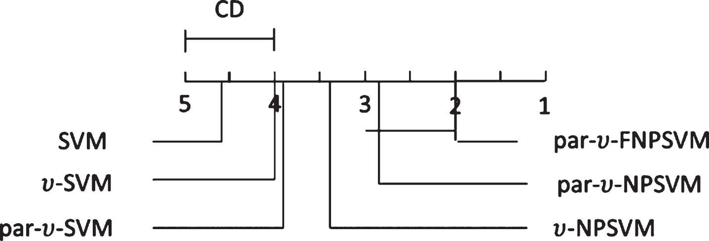
Comparison of the par-υ-FNPSVM against other five comparing algorithms with the Bonferroni-Dunn test.

5 Conclusion

In order to make υ-NPSVM take into account non-uniform noise and reduce the influence of noise, this paper adds parameter margin and fuzzy membership degree of nearest neighbor chain to υ-NPSVM and establishes par-υ-FNPSVM. In the numerical experiments on UCI data sets, the new model has achieved good classification F1 score, and the training time has not changed significantly. This shows that the new algorithm is indeed superior in dealing with problem of heteroscedastic noises and reducing the influence of noises.

When adding the parameter margin, it is necessary to calculate the parameter margin loss function; when adding the nearest neighbor fuzzy membership degree, it is necessary to optimize the selection of the parameters for membership degree. Although the establishment of parameter-margin loss function and the method of grid optimization can improve the classification F1 score and find the ideal parameters, both tasks require a certain amount of calculation time. In other words, the improvement of classification F1 score comes at the cost of parameter optimization time. Therefore, how to quickly and effectively select the best parameters is a problem for further study.

Footnotes

Appendix 1

For problem (19), we introduce its Lagrangian function $\begin{matrix} L (w_{+}, b_{+}, u_{+}, d_{+}, ɛ_{+}, ξ_{-}, α, β, γ, θ^{(1) \sim (5)}) \\ = \frac{1}{2} {∥ w_{+} ∥}^{2} + C_{1} (v_{1} ɛ_{+} + \frac{1}{p} \sum_{i = 1}^{p} s_{i} (η_{i} + η_{i}^{*})) \\ + (- v_{2} (\frac{1}{2} {∥ u_{+} ∥}^{2} + d_{+}) + \frac{1}{q} \sum_{j = p + 1}^{p + q} s_{j} ξ_{j}) \\ + \sum_{i = 1}^{p} α_{i} ((w_{+} \cdot x_{i}) + b_{+} - ɛ_{+} - η_{i}) \\ + \sum_{i = 1}^{p} β_{i} (- (w_{+} \cdot x_{i}) - b_{+} - ɛ_{+} - η_{i}^{*}) \\ + \sum_{j = p + 1}^{p + q} γ_{i} ((w_{+} \cdot x_{j}) + b_{+} + u_{+} x_{i} + d_{+} - ξ_{j}) \\ - \sum_{i = 1}^{p} θ_{i}^{(1)} η_{i} - \sum_{i = 1}^{p} θ_{i}^{(2)} η_{i}^{*} - \sum_{j = p + 1}^{p + q} θ_{j}^{(3)} ξ_{j} \\ - θ^{(4)} d_{+} - θ^{(5)} ɛ_{+} \end{matrix}$ where α = (α₁, …, α_p) ^T, β = (β₁, …, β_p) ^T, γ = (γ₁, …, γ_p) ^T, $θ^{(i)} = (θ_{1}^{(i)}, \dots, θ_{p}^{(i)})^{T}, i = 1, 2, θ^{(3)} = (θ_{p + 1}^{(3)}, \dots, θ_{p + q}^{(3)})^{T},$ θ⁽⁴⁾ ∈ R⁺, θ⁽⁵⁾ ∈ R⁺ are the Lagrangian multipliers.

For w₊, b₊, u₊, d₊, ɛ₊, ξ_-, we use the Karush-Kuhn-Tucker (KKT) necessary and sufficient optimality conditions to get the following equations $\nabla_{w_{+}} L = w_{+} + \sum_{i = 1}^{p} α_{i} x_{i} - \sum_{i = 1}^{p} β_{i} x_{i} + \sum_{j = p + 1}^{p + q} γ_{j} x_{j}$ $\nabla_{b_{+}} L = \sum_{i = 1}^{p} α_{i} - \sum_{i = 1}^{p} β_{i} + \sum_{j = p + 1}^{p + q} γ_{j} = 0$ $\nabla_{u_{+}} L = - v_{2} u_{+} + \sum_{j = p + 1}^{p + q} γ_{j} x_{j} = 0$ $\nabla_{d_{+}} L = - v_{2} + \sum_{j = p + 1}^{p + q} γ_{j} - θ^{(4)} = 0$ $\nabla_{ɛ_{+}} L = C_{1} v_{1} - \sum_{i = 1}^{p} α_{i} - \sum_{i = 1}^{p} β_{i} - θ^{(5)} = 0$ $\begin{array}{l} \nabla_{η_{+}} L = \frac{s_{i} C_{1}}{p} e - α - θ^{(1)} = 0 \\ \nabla_{η_{+}^{*}} L = \frac{s_{i} C_{1}}{p} e - β - θ^{(2)} = 0 \\ \nabla_{ξ_{-}} L = \frac{s_{j}}{q} e - γ - θ^{(3)} = 0 \end{array}$ From these equations, we get $w_{+} = - \sum_{i = 1}^{p} α_{i} x_{i} + \sum_{i = 1}^{p} β_{i} x_{i} - \sum_{j = p + 1}^{p + q} γ_{j} x_{j}$ $u_{+} = \frac{1}{v_{2}} \sum_{j = p + 1}^{p + q} γ_{j} x_{j}$ $\begin{array}{l} \sum_{i = 1}^{p} α_{i} = \sum_{i = 1}^{p} β_{i} + \sum_{j = p + 1}^{p + q} γ_{j} - v_{2} + \sum_{j = p + 1}^{p + q} γ_{j} ⩾ 0 \\ C_{1} v_{1} - \sum_{i = 1}^{p} α_{i} - \sum_{i = 1}^{p} β_{i} ⩾ 0 \\ 0 ⩽ α ⩽ \frac{s_{i} C_{1}}{p} e_{+} \\ 0 ⩽ β ⩽ \frac{s_{i} C_{1}}{p} e_{+} \\ 0 ⩽ γ ⩽ \frac{s_{j}}{q} e_{-} \end{array}$ where e₊ = (1, . . . , 1) ^T ∈ R^p and e_- = (1, . . . , 1) ^T ∈ R^q.

Then, using (19) and the above K.K.T conditions, we can obtain the Wolfe dual problem (21).

Appendix 2

For problem (20), we introduce its Lagrangian function $\begin{matrix} L (w_{+}, b_{+}, u_{+}, d_{+}, ɛ_{+}, ξ_{-}, α, β, γ, θ^{(1) \sim (5)}) \\ = \frac{1}{2} {∥ w_{-} ∥}^{2} + C_{3} (v_{3} ɛ_{-} + \frac{1}{q} \sum_{i = p + 1}^{p + q} s_{i} (η_{i} + η_{i}^{*})) \\ + (- v_{4} (\frac{1}{2} {∥ u_{-} ∥}^{2} + d_{-}) + \frac{1}{p} \sum_{j = 1}^{p} s_{j} ξ_{j}) \\ + \sum_{i = p + 1}^{p + q} α_{i} ((w_{-} \cdot x_{i}) + b_{+} - ɛ_{+} - η_{i}) \\ + \sum_{i = p + 1}^{p + q} β_{i} (- (w_{-} \cdot x_{i}) - b_{-} - ɛ_{-} - η_{i}^{*}) \\ - \sum_{j = p + 1}^{p + a} γ_{i} ((w_{-} \cdot x_{j}) + b_{+} - u_{-} x_{i} - d_{-} + ξ_{j}) \\ - \sum_{i = p + 1}^{p + q} θ_{i}^{(1)} η_{i} - \sum_{i = p + 1}^{p + q} θ_{i}^{(2)} η_{i}^{*} - \sum_{j = 1}^{p} θ_{j}^{(3)} ξ_{j} \\ - θ^{(4)} d_{-} - θ^{(5)} ɛ_{-} \end{matrix}$ where α = (α_p+1, …, α_p+q) ^T, β = (β_p+1, …, β_p+q) ^T, $θ^{(i)} = {(θ_{p + 1}^{(i)}, \dots, θ_{p + q}^{(i)})}^{T}, i = 1, 2$ , $θ^{(3)} = {(θ_{1}^{(3)}, \dots, θ_{p}^{(3)})}^{T}$ , θ⁽⁴⁾ ∈ R⁺, θ⁽⁵⁾ ∈ R⁺ are the Lagrangian multipliers.

For w₊, b₊, u₊, d₊, ɛ₊, ξ_-, we use the Karush-Kuhn-Tucker (KKT) necessary and sufficient optimality conditions to get the following equations $\nabla_{-} L = w_{-} + \sum_{i = p + 1}^{p + q} α_{i} x_{i} - \sum_{i = p + 1}^{p + q} β_{i} x_{i} - \sum_{j = 1}^{p} γ_{j} x_{j}$ $\nabla_{b_{-}} L = \sum_{i = p + 1}^{p + q} α_{i} - \sum_{i = p + 1}^{p + q} β_{i} - \sum_{j = 1}^{p} γ_{j} = 0$ $\nabla_{u_{-}} L = - v_{4} u_{-} + \sum_{j = 1}^{p} γ_{j} x_{j} = 0$ $\nabla_{d_{+}} L = - v_{4} + \sum_{j = 1}^{p} γ_{j} - θ^{(4)} = 0$ $\nabla_{ɛ_{-}} L = C_{3} v_{3} - \sum_{i = p + 1}^{p + q} α_{i} - \sum_{i = p + 1}^{p + q} β_{i} - θ^{(5)} = 0$ $\begin{array}{l} \nabla_{η_{-}} L = \frac{s_{i} C_{3}}{q} e - α - θ^{(1)} = 0 \\ \nabla_{η_{-}^{*}} L = \frac{s_{i} C_{3}}{q} e - β - θ^{(2)} = 0 \\ \nabla_{ξ_{+}} L = \frac{s_{j}}{p} e - γ - θ^{(3)} = 0 \end{array}$ From these equations, we get $w_{-} = - \sum_{i = p + 1}^{p + q} α_{i} x_{i} - \sum_{i = p + 1}^{p + q} β_{i} x_{i} + \sum_{j = 1}^{p} γ_{j} x_{j}$ $u_{-} = \frac{1}{v_{4}} \sum_{j = p + 1}^{p + q} γ_{j} x_{j}$ $\sum_{i = 1}^{p} α_{i} = \sum_{i = 1}^{p} β_{i} + \sum_{j = p + 1}^{p + q} γ_{j} - v_{4} + \sum_{j = 1}^{p} γ_{j} ⩾ 0$ $\begin{array}{l} C_{3} v_{3} - \sum_{i = p + 1}^{p + q} α_{i} - \sum_{i = p + 1}^{p + q} β_{i} ⩾ 0 \\ 0 ⩽ α ⩽ \frac{s_{i} C_{3}}{q} e_{-} \\ 0 ⩽ γ ⩽ \frac{s_{j}}{p} e_{+} \end{array}$ where e₊ = (1, . . . , 1) ^T ∈ R^p and e_- = (1, . . . , 1) ^T ∈ R^q.

Then, using (20) and the above K.K.T conditions, we can obtain the Wolfe dual problem (29).

References

Barnes

and Hunt

, E-commerce and v-business [M], London: Routledge, 2012.

, Medo

and Yeung

, Recommender systems [J], Physics Reports 519 (2012), 1–49.

Vapnik

V.N.

, Estimation of dependences based on empirical data, Springer Vcrlag, New York, 1982.

Vapnik

V.N.

, The nature of statistical learming theory, New York, Springer, 1995.

Jinbo

and Vapnik

V.N.

, Learning with rigorous support vector machines[J], Learning Theory and Kernel Machines, 2003, 243–257.

Wenqing

, Yinaer

and Nan

, Support vector machine based machine learning method for GS 8QAM constellation classification in seamless integrated fiber and visible light communication system[J], Science China(Information Sciences) 63(10) (2020), 182–193.

Lawi

and Aziz

, Classification of Credit Card Default Clients Using LS-SVM Ensemble, 2018 Third International Conference on Informatics and Computing (ICIC), Palembang, Indonesia, 2018, pp. 8780427.

, Lyu

, Han

, et al., An SVM Approach for Five-Phase Current Source Converters Output Current Harmonics and Common-Mode Voltage Mitigation[J], IEEE Transactions on Industrial Electronics 67(7) (2020), 5232–5245.

Yasoda

, Ponmagal

R.S.

, Bhuvaneshwari

K.S.

, et al., Automatic detection and classification of EEG artifacts using fuzzy kernel SVM and wavelet ICA (WICA)[J], Soft Computing, 2020, 1–9.

10.

Rizwan-ul-Hassan,

Changgang L.

and Yutian

, Online dynamic security assessment of wind integrated power system using SDAE with SVM ensemble boosting learner[J], International Journal of Electrical Power & Energy Systems 125 (2021), 106429.

11.

Xiangyang

, Ting

and Juan

, Color image segmentation using pixel wise support vector machine classification, Pattern Recogn 44(4) (2011), 777–787.

12.

Khan

N.M.

, Ksantini

, Ahmad

I.S.

, et al., A novel SVM+NDA model for classification with an application to face recognition, Pattern Recogn 45(1) (2012), 66–79.

13.

Mangasarian

O.L.

and Wild

E.W.

, Multisurface Proximal Support Vector Machine Classification via Generalized Eigenvalues, IEEE Transactions on Pattern Analysis & Machine Intelligence 28(1) (2006), 69–74. DOI: 10.1109/TPAMI.2006.17

14.

Chen

, Yang

, Shao

, Chen Ju

, & Zhang

and Jing

, A Trace Lasso Regularized Robust Nonparallel Proximal Support Vector Machine for Noisy Classification, IEEE Access, 2019, 1–1. DOI:10.1109/ACCESS.2019.2893531.

15.

, Ren

, Shao

, Ye

and Guo

, Generalized elastic net Lp-norm nonparallel support vector machine, Engineering Applications of Artificial Intelligence 88 (2020). DIO: 10.1016/j.engappai.2019.103397.

16.

Jayadeva,

R. Khemchandani

and Chandra

, Twin support vector machines for pattern classification, IEEE Trans Pattern Anal Mach Intell, IEEE Transactions on Pattern Analysis and Machine Intelligence 29(5) (2007), 905–910. DOI: 10.1109/TPAMI.2007.1068

17.

Xie

and Xu

, An efficient regularized K-nearest neighbor structural twin support vector machine, Appl Intell 49 (2019), 4258–4275. DOI: 10.1007/s10489-019-01505-5

18.

Lima

M.D.D.

, Lima

J.D.O.R.E.

and Barbosa

R.M.

, Medical data set classification using a new feature selection algorithm combined with twin-bounded support vector machine, Med Biol Eng Comput 58 (2020), 519–528. DOI: 10.1007/s11517-019-02100-z

19.

Yingjie

, Zhiquan

and Dalian

, Efficient sparse nonparallel support vector machines for classification, Neural Comput Appl, 2012, 1007–1331.

20.

Yingjie

, Zhiquan

and Dalian

, υ-Nonparallel support vector machine for pattern classification, Neural Computing and Applications 25(5) (2014), 1007–1020.

21.

Liang-Liang

and Jian

, Assessment Model of Command Information System Security Situation Based on Twin Support Vector Machines[J], Fire Control & Command Control, 2017.

22.

Liang-Liang

and Jian

, Assessment Model of Command Information System Security Situation Based on Twin Support Vector Machines[J], Fire Control & Command Control, 2017.

23.

Yuanhai

and Naiyang

, A novel margin-based twin support vector machine with unity norm hyperplanes, Neural Comput Appl 22 (2013), 1627–1635.

24.

Zhiquan

, Yingjie

and Yong

, Structural twin support vector machine for classification, Knowl-Based Syst 43 (2013), 74–81.

25.

Yingjie

, Yong

and Xiaohui

, Recent advances on support vector machines research, Technol Econ Dev Econ 18 (2012), 5–33.

26.

Zhensong

, Zhiquan

, Bo

, et al., Learning with label proportions based on nonparallel support vector machines[J], Knowledge-Based Systems 119(MAR.) (2017), 126–141.

27.

Yingjie

, Xuchan

and Yong

, A divide-and-combine method for large scale nonparallel support vector machines[J], Neural Netw 75 (2016), 12–21.

28.

Liming

, Maoxiang

, Rongfen

, et al., A nonparallel support vector machine with pinball loss for pattern classification[J], Journal of Intelligent and Fuzzy Systems 39(1) (2020), 1–13.

29.

Yingjie

, Zhiquan

and Dalian

, υ-Nonparallel support vector machine for pattern classification, Neural Computing and Applications 25(5) (2014), 1007–1020.

30.

Peiyi

, Lungbiao

and Minshiu

, A new support vector classification algorithm with parametric-margin model[C], Neural Networks, IJCNN 2008, (IEEE World Congress on Computational Intelligence), IEEE International Joint Conference on. IEEE, 2008, 420–425.

31.

Chihchung

and Chihjen J

, Training v-support vector regression: theory and algorithms[J], Neural Computation 14(8) (2002), 1959–1977.

32.

Fayang

, Jian

, et al., Extended nearest neighbor chain induced instance-weights for SVMs, Pattern Recognition 60 (2016), 863–874.

33.

Demiar

and Schuurmans

, Statistical Comparisons of Classifiers over Multiple Data Sets, Journal of Machine Learning Research 7(1) (2006), 1–30.