Connectivity parameters have a crucial role in the study of different networks in the physical world. The notion of connectivity plays a key role in both theory and application of different graphs. In this article, a prime idea of connectivity concepts in intuitionistic fuzzy incidence graphs (IFIGs) with various examples is examined. IFIGs are essential in interconnection networks with influenced flows. Therefore, it is of paramount significance to inspect their connectivity characteristics. IFIGs is an extended structure of fuzzy incidence graphs (FIGs). Depending on the strength of a pair, this paper classifies three different types of pairs such as an α - strong, β - strong, and δ-pair. The benefit of this kind of stratification is that it helps to comprehend the fundamental structure of an IFIG thoroughly. The existence of a strong intuitionistic fuzzy incidence path among vertex, edge, and pair of an IFIG is established. Intuitionistic fuzzy incidence cut pairs (IFICPs) and intuitionistic fuzzy incidence trees (IFIT) are characterized using the idea of strong pairs (SPs). Complete IFIG is defined, and various other structural properties of IFIGs are also investigated. The proof that complete IFIG does not contain any δ-pair is also provided. A real-life application of these concepts related to the network of different computers is also provided.
In 1736, Euler first proposed the idea of graph theory. In the history of mathematics, the solution provided by Euler of the famous Konigsberg bridge problem is considered to be the first theorem of graph theory. The graph concept is one of the most excellent and widely employed tools for multiple real-world problem representation, modeling, and analysis. To indicate the objects and their relations between themselves, the graph vertices or nodes and edges or arcs are applied, respectively. The idea of the graph is a handy tool for solving combinatorial problems in different areas such as geometry, algebra, number theory, topology, operations research, optimization, and computer science. Gurevich [10] discussed classes of infinite loaded graphs with randomly deleted edges.
There is a drawback of graphs because they are silent when there are unpredictability and vagueness among relationships of different objects. This disadvantage of graphs makes way for Rosenfeld [30] to present an excellent idea of fuzzy graphs (FGs). The study of FGs opens a new door for many researchers to take part in this field, such as Bhutani and Rosenfeld [6] discussed strong arcs in FGs. Later, Mathew and Sunitha [15] examined three types of arcs depending on the strength of the arcs, such as α - strong, β - strong, and δ - arc. Poulik and Ghorai [28] introduced the Wiener index for a bipolar fuzzy graph (BFG) along with its certain properties. They also created the term Wiener absolute index based on the total accurate connectivity between all the pair of vertices and in the whole BFG. They talked about the behavior of Wiener absolute index in various BFGs such as bipolar fuzzy forest, bridge, and tree. Characterization of bipolar fuzzy detour g-eccentric node, bipolar fuzzy detour g-boundary nodes, and bipolar fuzzy detour g-interior nodes in a BFG was examined by Poulik and Ghorai [24]. They also explored some properties of bipolar fuzzy detour g-boundary nodes, bipolar fuzzy detour g-interior nodes, and bipolar fuzzy complete nodes. They also provided an application of detour g-distance, detour g-boundary node, detour g-interior node. Poulik and Ghorai [25] presented different types of indices like connectivity index and average connectivity index of BFG. They also initiated an idea of different types of nodes like bipolar fuzzy connectivity-enhancing node, bipolar fuzzy connectivity-reducing node, and bipolar fuzzy connectivity-neutral node with their properties. Poulik et al. [27] applied an interval-valued fuzzy graph (IVFG) and degree of vertices for performance evaluation in an educational system. They also provided a real-life application using IVFG in the education system in Taiwan. Poulik and Ghorai [26] presented a note on BFGs with an application.
Fuzzy sets (FSs) have some limitations; they give the degree of membership of an element in a given set but do not give any clue about the degree of non-membership of an element in a set. This deficiency in FSs, encourages Atanassov [5] to initiate the notion of intuitionistic fuzzy sets (IFSs). IFSs give both a degree of membership and a degree of non-membership, which are more or less independent of each other; the only requirement is that the sum of these two degrees is not greater than 1. Shannon and Atanassov [32] introduced intuitionistic fuzzy graphs (IFGs) as a generalization of FGs. Later, many researchers worked on IFGs such as Parvathi, and Karunambigai [23] gave certain properties of IFGs. Akram and Davvaz [2] proposed an innovative idea of strong IFGs, self-complementary, and self weak complementary strong IFGs. Akram and Alshehri [1] introduced various types of intuitionistic fuzzy bridges, intuitionistic fuzzy cut-vertices, intuitionistic fuzzy cycles, intuitionistic fuzzy trees in IFGs and investigate some of their interesting properties. Akram and Dudek [3] determined different properties of the sequence of crisp structures that characterize a given property of the intuitionistic fuzzy structure. Alshehri and Akram [4] applied IFSs to multi-graphs, planar graphs, and dual graphs along with their magnetic properties. They also presented an idea of isomorphism between intuitionistic fuzzy planar graphs. For a more deep and comprehensive study on IFGs, we may suggest to the reader [11, 31].
FGs and IFGs cannot give any hint of the impact of a vertex on edge. This deficiency in FGs and IFGs caused to the introduction of FIGs. Dinesh [8] was the first who introduced the fundamental idea of FIGs. Mordeson and Mathew [16] developed a relationship between weak incidence pairs and fuzzy incidence end nodes. Fang et al. [9] presented the idea of connectivity index and Wiener index of FIGs. Malik et al. [12] applied FIGs to the problems involving human trafficking. Mathew et al. [13] proposed an idea of node connectivity and arc connectivity in FIGs. Their relationships with fuzzy connectivity parameters are obtained. Mordeson et al. [17] initiated the notion of a vague incidence graph and its eccentricity. They applied the results to problems including illegal immigration and illegal transfer of people. Mordeson et al. [18] introduced the notion of the degree of incidence of a vertex and an edge in a FG theory. They concentrated on incidence, where the edge is adjacent to the vertex. They examined results related to bridges, cut vertices, cut pairs, fuzzy incidence paths, fuzzy incidence trees for FIGs. For a more detailed study on FIGs, we may refer to the reader [7]. The idea of order, size, domination, strong fuzzy incidence domination, weak fuzzy incidence domination, and a relationship between strong fuzzy incidence domination and weak fuzzy incidence domination for FIGs were presented by Nazeer et al. [20]. Nazeer et al. [21] proposed the idea of domination in the join of FIGs along with an application in the trading system of different countries. Nazeer and Rashid [22] introduced Picture FIGs. A variety of operations in IFIGs, including Cartesian product (CP), composition, tensor product, and normal product, were proposed by Nazeer et al. [19]. They also discussed the application of CP and the composition of two IFIGs in the textile industry.
Mathew and Mordeson [14] presented connectivity concepts in FIGs such as α-SP, β-SP, δ pair, fuzzy incidence tree, and fuzzy incidence cycle. This motivates us to introduce these ideas for IFIGs because these concepts are unknown for IFIGs. In the future, these ideas will help us to study the different properties of IFIGs in detail. The IFIG is a more realistic approach than FIGs because of the degree of non-membership.
The remainder of this article is formulated as follows. Section 2 provides some preliminary results which are required to understand the remaining part of the article. The elementary concepts and notions of IFIGs are discussed in Section 3. In Section 4, some results of connectivity in IFIG with numerical examples are proved. Section 5 contains a real-life application of the network of different computers. Conclusions and prospects are elaborated in Section 6.
Preliminaries
Definition 2.1. [20] A mapping μ : T → [0, 1] is named as a fuzzy subset (FSS) of T. A FG with M as the underlying set is a pair G = (σ, χ), where σ : M → [0, 1] is FSS, χ : M × M → [0, 1] is a fuzzy relation on the FSS σ such that χ (a, b) ≤ σ (a) ∧ σ (b) for each a, b ∈ M, and M is a finite set.
Definition 2.2. [14] Let be a graph. Then is an incidence graph, where .
Definition 2.3. [14] Let be a graph and η be a FSS of , ϑ be a FSS of and κ be a FSS of . If κ (v, e) ≤ η (v) ∧ ϑ (e) for each and , then κ is known as fuzzy incidence of .
Definition 2.4. [14] Let be a graph and (η, ϑ) be a fuzzy subgraph of . If κ is a fuzzy incidence of , then is a FIG of . FIG is given in Fig 2.
Definition 2.5. [23] An IFG is where η = (η1, η2) , ϑ = (ϑ1, ϑ2) and
such that where η1 (vk) represents the grade of membership and where η2 (vk) represents the grade of non-membership of the vertex and 0 ≤ η1 (vk) + η2 (vk) ≤1 for every .
where ϑ1 (vk, vi) represents the grade of membership and where ϑ2 (vk, vi) represents the grade of non-membership of the edge ϑ2 (vk, vi) such that ϑ1 (vk, vi) ≤ ⊖ {η1 (vk) , η1 (vi)} and ϑ2 (vk, vi) ≤ ⊕ {η2 (vk) , η2 (vl)} and 0 ≤ ϑ1 (vk, vi) + ϑ2 (vk, vi) ≤1 for every , ⊕ and ⊖ are used for the maximum and minimum operators, respectively.
Definition 2.6. [19] Let be a graph and be a fuzzy incidence graph of . Then is known as an IFIG of where η = (η1, η2) , ϑ = (ϑ1, ϑ2) and κ = (κ1, κ2).
such that and , where η1 and η2 represent the membership (MS) value and non-membership (NMS) value of the vertex respectively and 0 ≤ η1 (vi) + η2 (vi) ≤1 for every
and , where ϑ1 (vi, vj) and ϑ2 (vi, vj) represent MS and NMS value of the edge (vi, vj) respectively such that ϑ1 (vivj) ≤ ⊖ {η1 (vi) , η1 (vj)}, ϑ2 (vivj) ≤ ⊕ {η2 (vi) , η2 (vj)} and 0 ≤ ϑ1 (vivj) + ϑ2 (vivj) ≤1 for every .
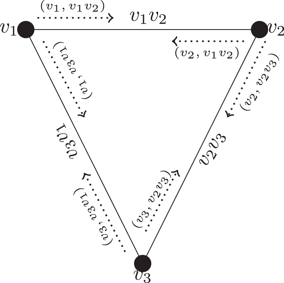
and , where κ1 (vi, vivj) and κ2 (vi, vivj) represent the MS and NMS value of the pair (vi, vivj) respectively such that ; κ1 (vi, vivj) ≤ ⊖ {η1 (vi) , ϑ1 (vivj)} , κ2 (vi, vivj)≤ ⊕ {η2 (vi) , ϑ2 (vivj)} and 0 ≤ κ1 (vi, vivj) + κ2 (vi, vivj) ≤1.
Note: In this work for the convenience we use instead of .
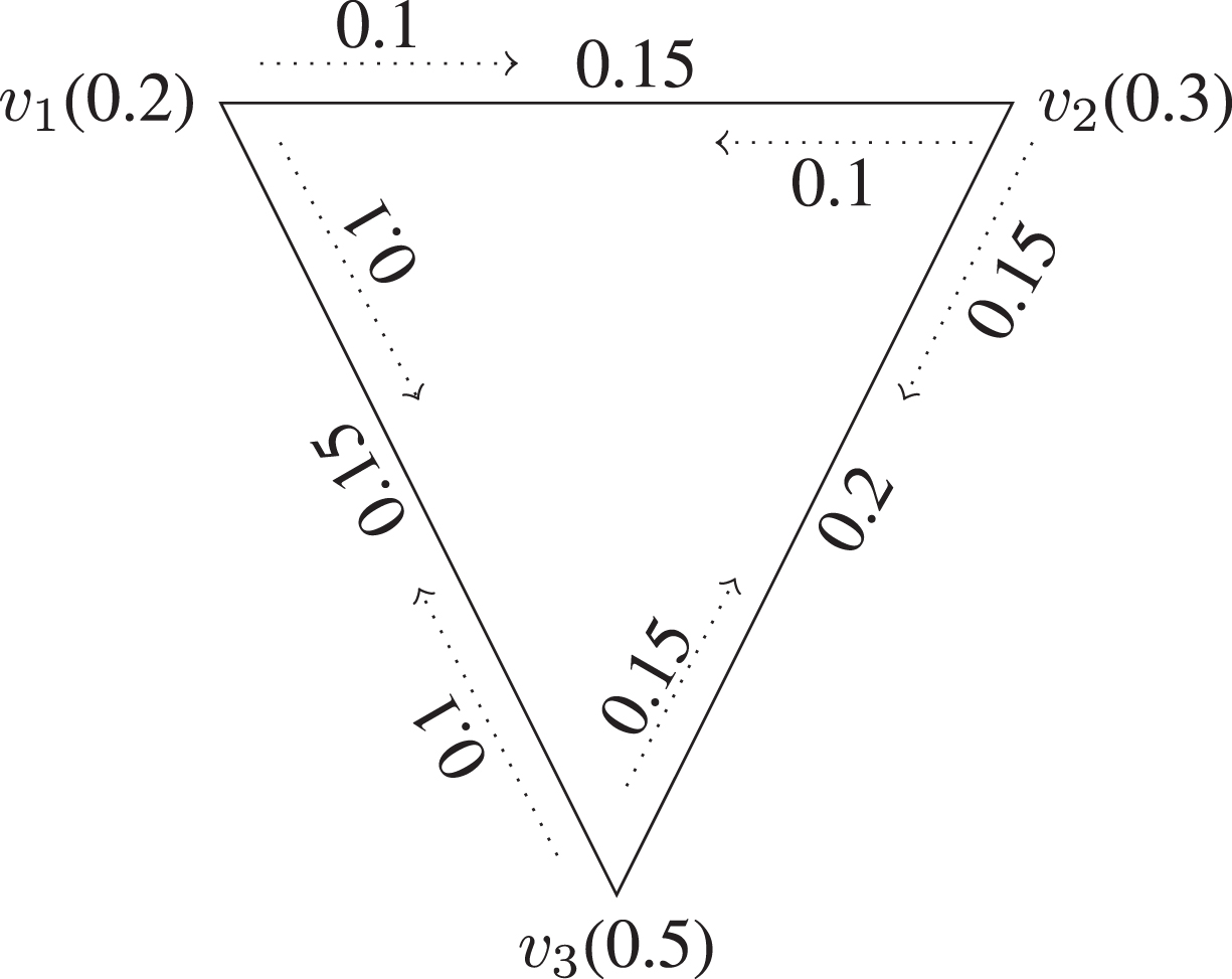
Example 2.7. Here, we include a daily life example of three different branches of hospitals. As an explanatory case, assume a network (IFIG) of three vertices expressing the distinct branches of a hospital. The MS value of the vertices denotes the percentage of patients who visit the hospital for their treatment of different diseases and the NMS value of the vertices indicates the percentage of patients who do not want to come to these hospitals due to their bad reputation. The MS value of the edges represents the percentage of those patients which one hospital recommends to another hospital due to the unavailability of doctors of different diseases in that hospital and the NMS value of the edges expresses the percentage of those patients which one hospital does not recommend to another hospital. The MS value of the pairs demonstrates the percentage of the profit of the hospital and the NMS value of the pairs shows the percentage of loss of the hospital.
Let be an IFIG associated with expressing three different branches of hospitals, where η (v) = (η1 (v) , η2 (v)), ϑ (uv) = (ϑ1 (uv) , ϑ2 (uv)), κ (v, uv) = (κ1 (v, uv) , κ2 (v, uv)) Let vertex set be and η (v1) = (0.2, 0.8), η (v2) = (0.3, 0.6), η (v3) = (0.5, 0.4). Then ϑ (v1v2) = (0.15, 0.7), ϑ (v2v3) = (0.2, 0.5), ϑ (v3v1) = (0.15, 0.6) and κ (v1, v1v2) = (0.1, 0.75), κ (v2, v1v2) = (0.1, 0.65), κ (v2, v2v3) = (0.15, 0.55), κ (v3, v2v3) = (0.15, 0.45), κ (v3, v3v1) = (0.1, 0.55), κ (v1, v3v1) = (0.1, 0.7). The corresponding IFIG is shown in Fig 3.
IFIG indicating three different branches of hospital.
Notions of intuitionistic fuzzy incidence graphs
In this section, some notions concerning IFIG with examples are explored. This section contains some of the ideas which are taken from [14]. We have proposed the concept of connected vertices. Also, we defined intuitionistic fuzzy incidence path (IFIP), intuitionistic fuzzy incidence strength (IFIS), intuitionistic fuzzy cycle (IFC), and intuitionistic fuzzy incidence cycle (IFIC) along with their examples. The idea of an intuitionistic fuzzy incidence subgraph is also provided. Three different kinds of pairs, along with examples, are also elaborated. Complete IFIG is also defined in this section.
Definition 3.1. For a vertex , if η1 (v) >0 and η2 (v) <1, then v is in support of η. For an edge , if ϑ1 (uv) >0 and ϑ2 (uv) <1, then uv is in support of ϑ, and for pair , if κ1 (u, uv) >0 and κ2 (u, uv) <1 then (u, uv) is in the support of κ. The support of η, ϑ and κ are represented as η∗, ϑ∗ and κ∗ respectively.
Definition 3.2. Let uv ∈ ϑ∗. Then uv is an edge of the IFIG and if (u, uv) , (v, uv) ∈ κ∗ then (u, uv) and (v, uv) are known as pairs of the IFIG.
Definition 3.3. [14] Two vertices vi and vj joined by an IFIP vi, (vi, vivi+1) , vivi+1, (vi+1, vivi+1) , vi+1, . . . , vj in an IFIG are known as connected.
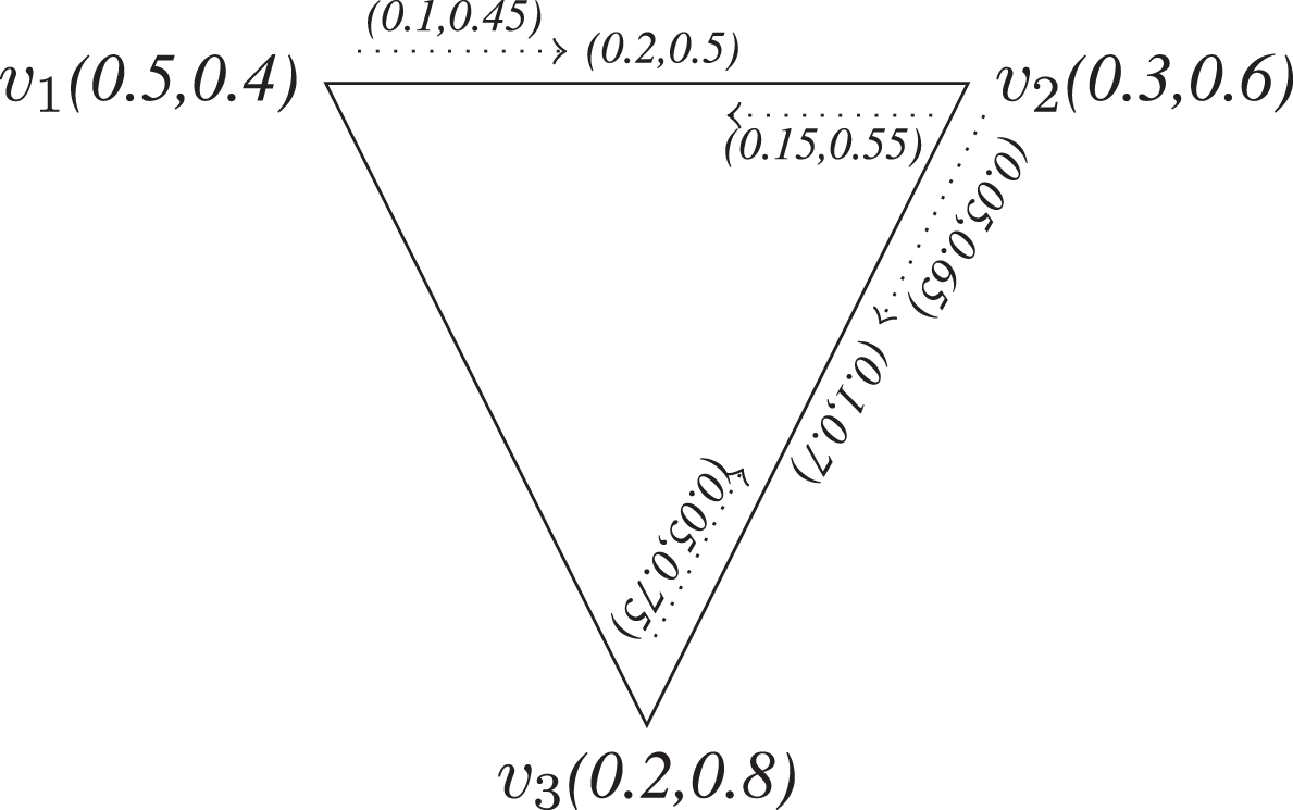
Example 3.4. Let be an IFIG associated with . Let vertex set be and η (v1) = (0.5, 0.4), η (v2) = (0.3, 0.6), η (v3) = (0.2, 0.8), ϑ (v1v2) = (0.2, 0.5), ϑ (v2v3) = (0.1, 0.7), and κ (v1, v1v2) = (0.1, 0.45), κ (v2, v1v2) = (0.15, 0.55), κ (v2, v2v3) = (0.05, 0.65), κ (v3, v2v3) = (0.05, 0.75).
It is clear from Fig. 4, v1, (v1, v1v2) , v1v2, (v2, v1v2) , v2 is an IFIP. Thus v1 and v2 are connected. Similarly, there are IFIPs between v2 to v3, i.e. v2, (v2, v2v3) , v2v3, (v3, v2v3) , v3 and v3 to v1, i.e.v1, (v1, v1v2) , v1v2, (v2, v1v2) , v2, (v2, v2v3) , v2v3, (v3, v2v3) , v3. Thus v2, v3 and v3, v1 are also connected.
Paths in IFIG.
Definition 3.5. An IFIS of an IFIG is defined as (⊖ κ1 (vi, vivj) , ⊕ κ2 (vi, vivj)); ∀ (vi, vivj) ∈ κ∗.
Definition 3.6. [14] The IFIG is a cycle, if (η∗, ϑ∗, κ∗) is a cycle and it is an IFC if (η∗, ϑ∗, κ∗) is a cycle and there exists no unique edge uv ∈ ϑ∗ s.t. ϑ (uv) = (⊖ ϑ1 (rs) , ⊕ ϑ2 (rs)); ∀rs ∈ ϑ∗.
Definition 3.7. [14] The IFIG is an IFIC if it is a fuzzy cycle and not exists a unique (u, uv) ∈ κ∗ s.t. κ (u, uv) = (⊖ κ1 (vi, vivj) , ⊕ κ2 (vi, vivj)); ∀ (vi, vivj) ∈ κ∗.
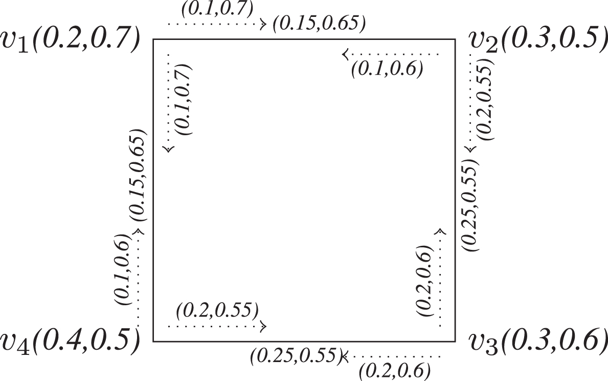
It is an IFC as there is no unique edge equal to the strength of the cycle. Since ϑ (v1v2) = ϑ (v1v4) = (0.15, 0.65). It is also an IFIC as there is no unique pair equal to the IFIS of . Since κ (v1, v1v2) = κ (v1, v1v4) = (0.1, 0.7).
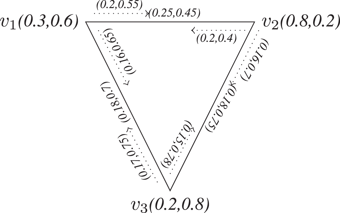
Example 3.9. Let be an IFIG as shown in Fig 6 with vertex set ϑ (v1v3) = (0.18, 0.7) , sϑ (v2v3) = (0.18, 0.75)and κ (v1, v1v2) = (0.2, 0.55) , κ (v2, v1v2) = (0.2, 0.4) , κ (v1, v1v3) = (0.16, 0.65) , κ (v3, v1v3) = (0.17, 0.75) , κ (v2, v2v3) = (0.16, 0.7) , κ (v3, v2v3)= (0.15, 0.78). It is not an IFIC because it has a unique pair (v3, v2v3) as κ (v3, v2v3) = (0.15, 0.78) = the IFIS of .
IFIG which is not a cycle.
Definition 3.10 [14] Let be an IFIG. Then is an intuitionistic fuzzy incidence subgraph of if υ ⊆ η, φ ⊆ ϑ and ω ⊆ κ such that υ1 (r) ≤ η1 (r), υ2 (r) ≥ η2 (r); , φ1 (rs) ≤ ϑ1 (rs), φ2 (rs) ≥ ϑ2 (rs); and ω1 (r, rs) ≤ κ1 (r, rs), ω2 (r, rs) ≥ κ2 (r, rs); .
An intuitionistic fuzzy incidence subgraph of is an intuitionistic fuzzy incidence spanning subgraph of if υ∗ = η∗.
Definition 3.11. Let be an IFIG. An IFIS of ρ is described as: κ (r, rs) = (⊖ κ1 (t, tu) , ⊕ κ2 (t, tu)); ∀ (t, tu) ∈ ρ .
where ρ is a IFIP between any two nodes, arcs and pairs belong to η∗, ϑ∗ and κ∗. The IFIS of the ρ from r to rs is denoted by .
Definition 3.12. Let be an IFIG. A pair (r, rs) is said to be a SP if κ1 (r, rs) ≥ ⊖ κ1 (t, tu) and κ2 (r, rs) ≤ ⊕ κ2 (t, tu); where represents the greatest IFIS of path r - rs.
Definition 3.13. A pair (r, rs) is called an α-SP if κ1 (r, rs) > ⊖ κ1 (t, tu) and κ2 (r, rs) < ⊕ κ2 (t, tu); .
Definition 3.14. A pair (r, rs) is called a β-SP if ; .
Definition 3.15. Let be an IFIG. A pair (r, rs) is called δ-pair if κ1 (r, rs) < ⊖ κ1 (t, tu) and κ2 (r, rs) > ⊕ κ2 (t, tu); .
Definition 3.16. [14] Let be an IFIG. An IFIP ρ in is called a strong if all of its pairs are strong.
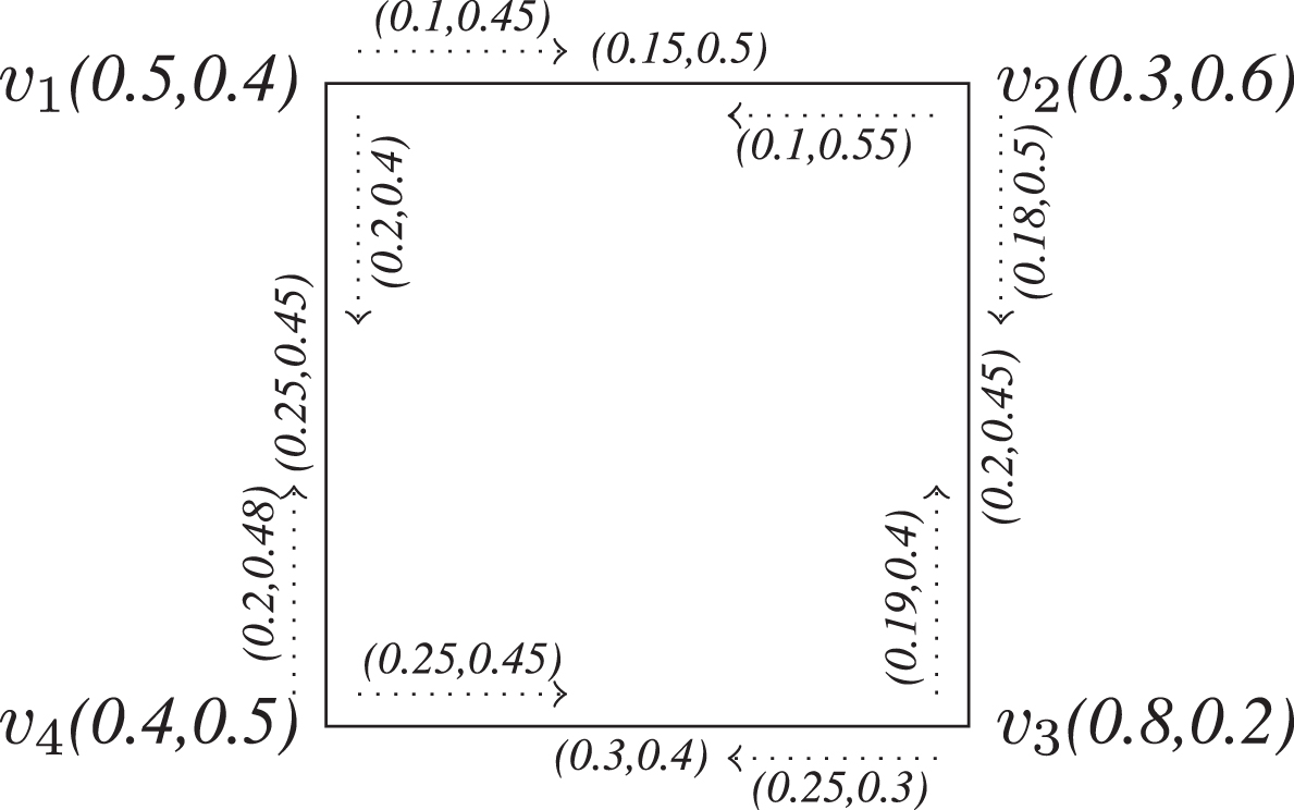
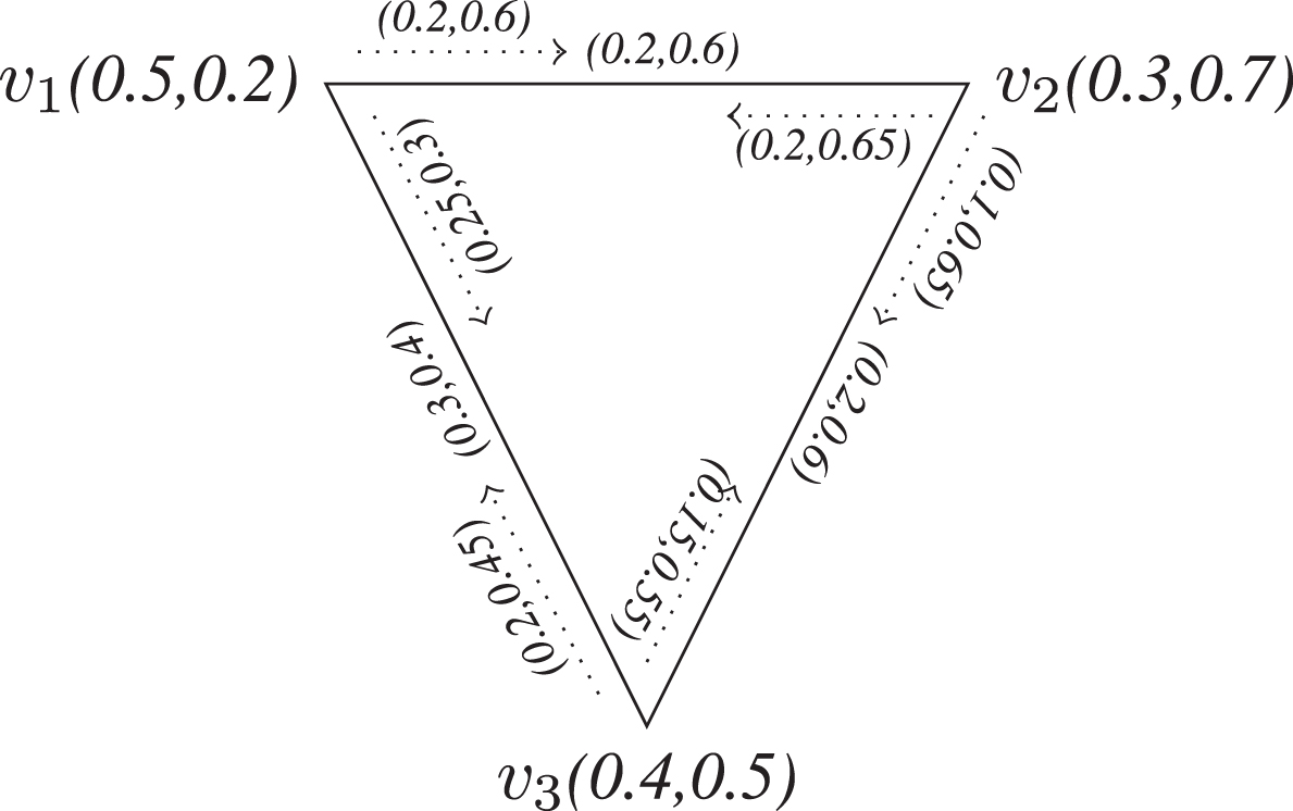
Example 3.17. Consider the IFIG as shown in Fig 7.
α-strong IFIP between (v2, v2v3) and v1.
All the vertices are α-strong except v2 as η1 (v2) =0.3 but ⊖η1 (vi) =0.4 > 0.3 and η2 (v2) =0.6 but ⊕η2 (vi) =0.5 < 0.6 . All the edges are α-strong except v1v2 as ϑ (v1v2) =0.15 but ⊖ϑ1 (vivj) =0.2 > 0.15 and ⊕ϑ2 (vivj) =0.45 < 0.5 . All the pairs are α-strong except (v1, v1v2) and (v2, v1v2) as ⊖κ1 (vi, vivj) =0.1 = κ1 (v1, v1v2) and ⊕κ2 (vi, vivj) =0.55 > 0.45 = κ2 (v1, v1v2); . Similarly we can see (v2, v1v2). Thus (v2, v2v3) , v2v3, (v3, v2v3) , v3, (v3, v3v4) , v3v4, (v4, v3v4) , v4, (v4, v1v4) , v1v4, (v1, v1v4) , v1 is an α-strong IFIP.
Definition 3.18. Let be an IFIG. An intuitionistic fuzzy incidence subgraph is called a subgraph of if υ1 (r) = η1 (r); ∀r ∈ υ∗, φ1 (rs) = ϑ1 (rs) , φ2 (rs) = ϑ2 (rs); ∀rs ∈ φ∗ and ω1 (r, rs) = κ1 (r, rs) , ω2 (r, rs) = κ2 (r, rs); ∀ (r, rs) ∈ ω∗.
Definition 3.19. Let be an IFIG. Then it is called an IFIT if there is a spanning subgraph of , that is a tree as for all pair (r, rs) ∈ κ∗ - ω∗, κ1 (r, rs) < ⊖ {κ1 (t, tu) | (t, tu) ∈ ω∗} and κ2 (r, rs) > ⊕ {κ2 (t, tu) | (t, tu) ∈ ω∗}. It can be stated as there is an IFIP in spanning subgraph from r to rs s.t. all of its pair has maximum κ1 MS value than κ1 (r, rs) and has minimum κ2 NMS value than κ2 (r, rs).
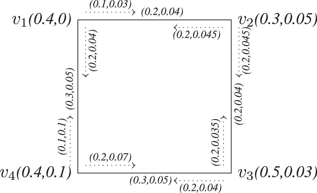
Example 3.20. Let be an IFIG given in Fig 8 with vertex set and η (v1) = (0.4, 0) , η (v2) = (0.3, 0.05) , η (v3) = (0.5, 0.03) , η (v4) = (0.4, 0.1) , ϑ (v1v2) = (0.2, 0.04) , ϑ (v1v4) = (0.3, 0.05) , ϑ (v2v3) = (0.2, 0.04) , ϑ (v3v4) = (0.3, 0.05) and κ (v1, v1v2) = (0.1, 0.03) , κ (v2, v1v2) = (0.2, 0.045) , κ (v1, v1v4) = (0.2, 0.04) , κ (v4, v1v4) = (0.1, 0.1) , κ (v2, v2v3) = (0.2, 0.045) , κ (v3, v2v3) = (0.2, 0.035) , κ (v3, v3v4) = (0.2, 0.04) , κ (v4, v3v4) = (0.2, 0.07).
IFIT.
The spanning subgraph of is the IFIG. It has the same MS and NMS value for all nodes, arcs and pairs, except for ω (d, da) = (0.18, 0.08) and ω (a, da) =0. Then (υ∗, φ∗, ω∗) is a tree. (a, da) ∈ κ∗ - ω∗. There is an IFIP: ϱ : da, (d, da) , d, (d, dc) , cd, (c, cd) , c, (c, cb) , bc, (b, bc) , b, (b, ba) , ab, (a, ab) , a with . But κ (a, da) = (0.1, 0.1) where 0.18 > 0.1 and 0.08 < 0.1. Hence, is an IFIT.
Definition 3.21. An IFIG is called complete if ϑ1 (vivj) = η1 (vi) ⊖ η1 (vj); ϑ2 (vivj) = η2 (vi) ⊕ η2 (vj) and κ1 (vi, vivj) = η1 (vi) ⊖ ϑ1 (vivj); κ2 (vi, vivj) = η2 (vi) ⊕ ϑ2 (vivj) for all (vi, vivj) ∈ κ∗.
Example 3.22. Let be an IFIG shown in Fig 9 with vertex set and η (v1) = (0.3, 0.6) , η (v2) = (0.4, 0.5) , η (v3) = (0.7, 0.3) , ϑ (v1v2) = (0.3, 0.6) , ϑ (v1v3) = (0.3, 0.6) ϑ (v2v3) = (0.4, 0.5) and κ (v1, v1v2) = (0.3, 0.6) κ (v2, v1v2) = (0.3, 0.6) , κ (v1, v1v3) = (0.3, 0.6) κ (v3, v1v3) = (0.3, 0.6) , κ (v2, v2v3) = (0.4, 0.5) κ (v3, v2v3) = (0.4, 0.5). It is a complete IFIG.
Complete IFIG.
Main results
In this section, we proved some important results on IFIGs. It is proved that every IFIC is always a strong cycle. Some novel results related to SPs are discussed. A very interesting result that every IFICP is a SP is also given in this section. The proof of an IFIT is always connected iff it does not contain any β-SP is also presented in this section. At the end of this section, a very fascinating result that a complete IFIG does not contain any δ-pair is provided.
Proposition 4.1.An IFIC is a strong cycle.
Proof. Consider an IFIC. Then by Definition 3.7, is a cycle so there does not exist the only rs ∈ ϑ∗ and pair (r, rs) ∈ κ∗ such that ϑ (rs) = (⊖ ϑ1 (tu) , ⊕ ϑ2 (tu)); ∀tu ∈ ϑ∗ and κ (r, rs) = (⊖ κ1 (t, tu) , ⊕ κ2 (t, tu)); ∀ (t, tu) ∈ κ∗.
Now we have to prove that each arc and pair in are strong. It is quite obvious that all arcs in a fuzzy cycle are strong. Let (r, rs) belongs to and assume that it is not strong. This implies (r, rs) is a δ-pair. Then by Definition 3.15, κ1 (r, rs) < ⊖ κ1 (t, tu) and κ2 (r, rs) > ⊕ κ2 (t, tu); where ; ∀ (t, tu) ∈ κ∗. As is a cycle so every pair in the incidence subgraph will have value κ1 (t′, t′u′) > ⊖ κ1 (t, tu) and κ2 (t′, t′u′) < ⊕ κ2 (t, tu); Which is a contradiction to our assumption that is an IFIC. Hence, (r, rs) is strong. ■
Proposition 4.2.Let be an IFIG and an intuitionistic fuzzy incidence subgraph of .Then ; ∀ (r, rs) ∈ ω∗
Proof. It is obvious because different r - rs IFIPs in may not be in or IFIPs have less IFIS in . ■
Proposition 4.3.Consider an IFIG. A pair (r, rs) ∈ κ∗ is a SP if κ (r, rs) = (⊖ κ1 (t, tu) , ⊕ κ2 (t, tu)); ∀ (t, tu) ∈ κ∗.
Proof. Since IFIS of r - rs IFIP in will has κ1 (r, rs) ≥ ⊖ κ1 (t, tu) and κ2 (r, rs) ≤ ⊕ κ2 (t, tu) where (t, tu) ∈ r - rs an IFIP.
If (r, rs) is the unique pair with κ1 (r, rs) = ⊖ κ1 (t, tu) and κ2 (r, rs) = ⊕ κ2 (t, tu) then all other IFIPs r - rs in will have IFIS: κ1 (r, rs) > ⊖ κ1 (t, tu) and κ2 (r, rs) < ⊕ κ2 (t, tu); . Hence, (r, rs) is an α-SP.
If pair (r, rs) is not the only pair then the possible greatest value for IFIS of an IFIP in will be κ (r, rs). ; . Thus, if there is an IFIP r - rs in with IFIS κ (r, rs). Then (r, rs) is β-strong. Otherwise (r, rs) is α-strong.
Therefore, from Case 1 and Case 2 it is clear that (r, rs) is a SP. ■
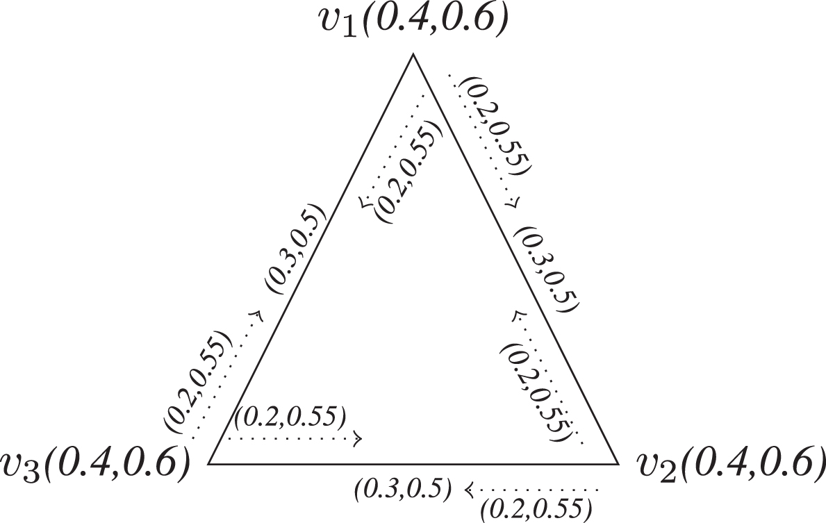
Example 4.4. Consider is an IFIG as given in the Fig 10 with vertex set and η (v1) = (0.4, 0.6) , η (v2) = (0.4, 0.6) , η (v3) = (0.4, 0.6) , ϑ (v1v2) = (0.3, 0.5) , ϑ (v1v3) = (0.3, 0.5) , ϑ (v2v3) = (0.3, 0.5) and κ (v1, v1v2) = (0.2, 0.55) , κ (v2, v1v2) = (0.2, 0.55) , κ (v1, v1v3) = (0.2, 0.55) , κ (v3, v1v3) = (0.2, 0.55) , κ (v2, v2v3) = (0.2, 0.55) , κ (v3, v2v3) = (0.2, 0.55).
Hence, is an IFIC which is strong because all the pairs in the Fig 10 are strong.
IFIG having all strong pairs.
Definition 4.5. Let be an IFIG. If the removal of a pair in an IFIG increases the number of connected components, then the pair is known as an IFICP.
Proposition 4.6.Let be an IFIG. A pair (r, rs) that is defined by κ (r, rs) = (⊖ {η1 (r) , ϑ1 (rs)} , ⊕ {η2 (r) , ϑ2 (rs)}) is strong.
Proof. Let be the intuitionistic fuzzy incidence subgraph of .
Suppose that is disconnected, then (r, rs) is an IFICP. But given κ (r, rs) = (κ1 (r, rs) , κ2 (r, rs)) = (⊖ {η1 (r) , ϑ1 (rs)} , ⊕ {η2 (r) , ϑ2 (rs)}). As is a subgraph of then κ1 (r, rs) = ⊖ {η1 (r) , ϑ1 (rs)} ≥ ⊖ {η1 (t) , ϑ1 (tu)} and
This shows that a pair (r, rs) is strong.
Now assume that is connected then there is a pair (r, rv) for some v ≠ r such that (r, rv) , (s, rs) ∈ ρ where ρ is an IFIP from r - rs in . Hence the IFIS of an IFIP ρ is: ⊖ {κ1 (r, rv) , κ1 (s, rs)} ≤ ⊖ {η1 (r) , ϑ1 (rv) , η1 (s) , ϑ1 (rs)} ≤ ⊖ {η1 (r) , ϑ1 (rs)} = κ1 (r, rs) ⇒κ1 (r, rs) ≥ ⊖ {κ1 (r, rv) , κ1 (s, rs)} and ⊕ {κ2 (r, rv) , κ2 (s, rs)} ≥ ⊕ {η2 (r) ϑ2 (rv) , η2 (s) , ϑ2 (rs)} ≥ ⊕ {η2 (r) , ϑ2 (rs)} = κ2 (r, rs) ⇒κ2 (r, rs) ≤ ⊕ {κ2 (r, rv) , κ2 (s, rs)}. Hence, (r, rs) is a SP.
The converse of the Proposition 4.6 is not true. In Fig 10 the pair (v1, v1v2) is strong. But κ1 (v1, v1v2) ≠ ⊖ {η1 (v1) , ϑ1 (v1v2)} and κ2 (v2, v1v2) ≠ ⊕ {η2 (v1) , ϑ2 (v1v2)}. ■
Example 4.7. Let be an IFIG. In Fig 11, only κ (v1, v1v2) = (⊖ {η1 (v1) , ϑ1 (v1v2)} ⊕ {η2 (v1) , ϑ2 (v1v2)})
Proof. Consider an IFIG and (r, rs) ∈ κ∗ be an IFICP. As is a subgraph of . Then ⊖ {η1 (r) , ϑ1 (rs)} ≥ ⊖ {η1 (r) , ϑ1 (rs)} and ⊕ {η2 (r) , ϑ2 (rs)} ≤ ⊕ {η2 (r) ϑ2 (rs)}; . Assume that (r, rs) is not a SP. Then κ1 (r, rs) < ⊖ {η1 (t) , ϑ1 (tu)} and κ2 (r, rs) > ⊕ {η2 (t) , ϑ2 (tu)}; . Let a strongest IFIP ϱ from r - rs in . Then ϱ with pair form an incidence cycle where (r, rs) is the weakest pair. But it is contradict our assumption, i.e. (r, rs) is an IFICP. Hence, (r, rs) is a SP. ■
Theorem 4.9.Let be a connected IFIG. Then there is a strong IFIP from any node r ∈ η∗ to any arc st ∈ ϑ∗.
Proof. As is connected, so ∃ an IFIP ϱ from r ∈ η∗ to st ∈ ϑ∗ such that ;(rn can be taken t also). Since κ (rk, rkrk+1) >0 ∀ k = 0, 1, 2, 3, . . . , n - 1 and κ (s, st) , κ (t, st) >0. Suppose that (rj-1, rj-1rj) is not a SP. Then (rj-1, rj-1rj) is δ-pair and it implies such that κ1 (rj-1, rj-1rj) < ⊖ {κ1 (rl-1, rl-1rl) | (rl-1, rl-1rl) ∈ κ∗} and κ2 (rj-1, rj-1uj) > ⊕ {κ2 (rl-1, rl-1rl) | (rl-1, rl-1rl) ∈ κ∗} Let ϱ be an IFIP from r to st in with IFIS . We observe that every pair in ϱ will have κ1 value greater than κ1 (rj-1, rj-1rj) and κ2 value smaller than κ2 (rj-1, rj-1rj). If ϱ is strong, then proof is completed. In other case, find out δ-pairs in ϱ and supersede these by IFIPs having strength more than κ1 and less than κ2 values. We will continue this procedure ultimately we will have an IFIP ς from r to st contain only SPs. ■
Theorem 4.10.Let be an IFIG. (r, rs) ∈ κ∗ is an IFICP iff it is α-strong.
Proof. As is an IFIG. Let (r, rs) ∈ κ∗ be an IFICP of . Then by Proposition 4.6, (r, rs) is an α-strong. i.e. κ1 (r, rs) > ⊖ {κ1 (t, tu) | (t, tu) ∈ κ∗} and κ2 (r, rs) < ⊕ {κ2 (t, tu) | (t, tu) ∈ κ∗} . Conversely, let (r, rs) be an α-strong. Then r, (r, rs) , rs is the unique strongest IFIP from r to rs. If a pair (r, rs) is removed from this IFIP then it will be reduced the IFIS between r and rs. Thus (r, rs) is an IFICP. ■
Theorem 4.11.Let be an IFIT. Any pair in κ∗ is strong iff it belongs to tree .
Proof. As is an IFIT. Let be the tree and (r, rs) be a strong pair in κ∗. Suppose that then
Since (r, rs) is strong,
. Since , as is a subgraph of . So above inequality(4.2) implies κ1 (r, rs) ≥ ⊖ {κ1 (t, tu) | (t, tu) ∈ κ∗}; ≥ ⊖ {κ1 (t, tu) | (t, tu) ∈ ω∗}; and κ2 (r, rs) ≤ ⊕ {κ2 (t, tu) | (t, tu) ∈ κ∗}; ≤ ⊕ {κ2 (t, tu) | (t, tu) ∈ ω∗}; a contradiction of inequality(4.1). Hence, . Conversely, let (r, rs) ∈ ω∗ then by Theorem 3.4 of [8], (r, rs) is an IFICP. This implies (r, rs) is strong. ■
Note:
The pairs of are the SPs of .
A pair (x, xy)∈ IFIT is strong iff (x, xy) is an IFICP.
The spanning tree can be gotten by eliminating all δ-pairs which are in cycles of .
The sum of κ MS values of the SPs of will be greater than the sum of ω MS values of and the sum of κ NMS values of the SPs of will be lesser than the sum of ω NMS values of , among all other spanning trees associated with .
Proposition 4.12.A connected IFIG is an IFIT iff it has no β-SPs.
Proof. Suppose is an IFIT. Then there is the only such that all pairs belong to are IFICPs so these pairs are α-strong. Thus, all pairs of , not belong to are δ-pairs (By Definition of an IFIT). Hence, there is no β-SP in . Conversely, assume that there is no β-SP in . Now we have to prove that is an IFIT.
If has no cycle, then is an IFIT.
If has cycle ξ. Then ξ has α-strong and δ-pairs only. But by Definition, all pairs of ξ cannot be α-strong. So there is a unique δ-pair in every cycle of .
Theorem 4.13.A connected IFIG is an IFIT iff there is a strong IFIP between any node arc pair. Particularly, this is an α-strong IFIP.
Proof. Let be an IFIT then there is a strong IFIP ξ between a node x ∈ η∗ and arc yz ∈ ϑ∗. By Theorem 4.8, ξ belongs to the corresponding maximum spanning tree of . As is a tree, so ξ is the only IFIP in . By Theorem 4.9 has no β-strong pairs. Thus, ξ is an α-strong IFIP. Conversely, suppose that is an IFIG and there is the only one α-strong IFIP between any node arc pair. Now assume that is not an IFIT then there is a cycle so for (r, rs) ∈ ϑ; κ1 (r, rs) ≥ ⊖ {κ1 (t, tu) | (t, tu) ∈ κ∗} and κ2 (r, rs) ≤ ⊕ {κ2 (t, tu) | (t, tu) ∈ κ∗} for all which shows that (r, rs) ∈ ϑ is a SP, which contradict the assumption that there is the only one strong IFIP between a node arc pair. Hence is an IFIT. ■
Proposition 4.14.Let be an IFIG and ξ be a strong IFIP between any node r and arc rs. Then ξ is a strongest r - rs path in the following cases.
ξ has only α-SPs.
ξ is the only one strong r - rs IFIP in .
All IFIPs r - rs in are of equal strength.
Proposition 4.15.A complete IFIG has no δ-pairs.
Proof. Suppose that a complete IFIG contains (r, rs) as a δ-pair. Then By Definition 3.15, κ1 (r, rs) < ⊖ κ1 (t, tu) and κ2 (r, rs) > ⊕ κ2 (t, tu); . Thus there is a stronger IFIP ξ in from r to rs. Suppose that (m, n) is the IFIS of ξ. If κ (r, rs) = κ (s, rs) = (p, q). So p < m and q > n. Every pair belongs to ξ will have κ1 MS value more than p and κ2 NMS value less than q. Let z be the first node in ξ next to r. Then κ1 (r, rz) > p and κ2 (r, rz) < q. But this is not possible because κ (r, rz) = (⊖ {η1 (r) , ϑ1 (rz)} , ⊕ {η2 (r) , ϑ2 (rz)}) = (p, q). Hence, there is no δ-pair in . Thus, in a complete IFIG, every pair is strong. ■
Real-life application
Here we include a real-life application of SPs of IFIGs. As an explanatory case, consider the network (IFIG) of five different computers. The vertices in a network are indicating five different computers. The MS value of the vertices represents the percentage of stored data in a computer system and the NMS value of the vertices expresses the empty space in a computer system. The MS values of the edges are representing the percentage of the total capacity of transfer of data among different computers and the NMS value of the edges is expressing the percentage of the total capacity of untransferable data among these computers. The MS value of the pairs is indicating the percentage of sharing data from one computer to another computer and the NMS value of the pairs is expressing the percentage of data that is not shareable from one computer to another computer. To transfer maximum data from one computer to another computer, the pairs should be strong either α-strong or β-strong because through SPs we can easily transfer maximum data from one computer to another computer. But in the case of non-SP (δ-pair) it will be difficult to share the huge amount of data from one computer to another computer.
Let be an IFIG shown in Fig. 12 expressing a network of different computers. Let vertex set be and η (C1) = (0.3, 0.5), η (C2) = (0.3, 0.7), η (C3) = (0.4, 0.3), η (C4) = (0.5, 0.5), η (C5) = (0.3, 0.2); ϑ (C1C2) = (0.3, 0.7), ϑ (C1C3) = (0.2, 0.4), ϑ (C1C5) = (0.2, 0.5), ϑ (C2C3) = (0.2, 0.5), ϑ (C3C4) = (0.3, 0.4), ϑ (C3C5) = (0.2, 0.2), ϑ (C4C5) = (0.1, 0.4), and κ (C1, C1C2) = (0.3, 0.7), κ (C2, C1C2) = (0.2, 0.6), κ (C1, C1C3) = (0.2, 0.4), κ (C3, C1C3) = (0.1, 0.3), κ (C1, C1C5) = (0.03, 0.4), κ (C5, C1C5) = (0.2, 0.5), κ (C2, C2C3) = (0.2, 0.6), κ (C3, C2C3) = (0.1, 0.4), κ (C3, C3C4) = (0.3, 0.4), κ (C4, C3C4) = (0.3, 0.4), κ (C3, C3C5) = (0.2, 0.3), κ (C5, C3C5) = (0.2, 0.2), κ (C4, C4C5) = (0.07, 0.4), κ (C5, C4C5) = (0.05, 0.3).
(v1, v1v2) a SP.
A network of different computers.
Since, κ1 (C1, C1C2) =0.3 > ⊖ κ1 (t, tu) =0.03 and κ2 (C1, C1C2) =0.7 ≰ ⊕ κ2 (t, tu) =0.6; . Therefore, κ (C1, C1C2) is not a SP. Similarly, κ (C1, C1C5) is not a SP. Now, κ1 (C2, C1C2) =0.2 > ⊖ κ1 (t, tu) =0.03 and κ2 (C2, C1C2) =0.6 < ⊕ κ2 (t, tu) =0.7; . Therefore, κ (C2, C1C2) is an α-SP. In the same way, κ (C1, C1C3), κ (C3, C1C3), κ (C5, C1C5), κ (C2, C2C3), κ (C3, C2C3), κ (C3, C3C4), κ (C4, C3C4), κ (C3, C3C5), κ (C5, C3C5), κ (C4, C4C5) and κ (C5, C4C5) are all an α-SPs. So, we can share the huge amount of data from one computer to another computer through all α-SPs. In this way, we can save time and energy.
Conclusion
IFIGs are studied and introduced in this paper. Their fundamental notions and properties are being established to comprehend the IFIGs comprehensively. SPs and strong IFIPs are founded in an IFIG. In a complete IFIG, every pair is a strong pair is discussed. The IFIG is a more realistic approach than FIGs because of the non-availability of the NMS degree in FIG, which is present in IFIG. Classification of pairs in IFIGs such as an α-strong, β-strong, and δ-pair is also examined. IFIGs are helpful to form vital networking and software programming. A real-life application of a network of different computers is also provided. In the future, our main ambition is to extend our work for soft IFIGs, Hamiltonian IFIGs, competition IFIGs, interval-valued IFIGs, threshold IFIGs, and bipolar IFIGs. Further work on these ideas will be reported in upcoming papers. The readers can work on the concept of domination, accurate domination, strong and weak domination in IFIGs. They can work on Wiener index and Wiener absolute index to compute boiling point of some molecular structures.
Footnotes
Acknowledgment
Authors are very thankful to the reviewers for their comments and suggestions to improve the quality of the manuscript.
References
1.
AkramM. and AlshehriN., Intuitionistic fuzzy cycles andintuitionistic fuzzy trees, The Scientific World Journal2014 (2014), 1–11.
2.
AkramM. and DavvazB., Strong intuitionistic fuzzy graphs, Filomat26(1) (2012), 177–196.
3.
AkramM. and DudekW.A., Intuitionistic fuzzy hypergraphs withapplications, Information Sciences218 (2013), 182–193.
4.
AlshehriN. and AkramM., Intuitionistic fuzzy planar graphs, Discrete Dynamics in Nature and Society2014 (2014), 1–9.
FangJ., NazeerI., RashidT. and LiuJ.B., Connectivity and Wiener Index of Fuzzy Incidence Graphs, Mathematical Problems in Engineering Article ID 6682966, (2021), 1–7.
10.
GurevichB., On classes of infinite loaded graphs with randomlydeleted edges, Applied Mathematics and Nonlinear Sciences5(2) (2020), 257–260.
11.
JiangL., ZhangT. and FengY., Identifying the critical factors ofsustainable manufacturing using the fuzzy DEMATEL method, Applied Mathematics and Nonlinear Sciences5(2) (2020), 391–404.
12.
MalikD.S., MathewS. and MordesonJ.N., Fuzzy incidence graphs:Applications to human trafficking, Information Sciences447 (2018), 244–255.
13.
MathewS., MordesonJ.N. and YangH.L., Incidence cuts andconnectivity in fuzzy incidence graphs, Iranian Journal ofFuzzy Systems16(2) (2019), 31–43.
14.
MathewS. and MordesonJ.N., Connectivity concepts in fuzzyincidence graphs, Information Sciences382 (2017), 326–333.
15.
MathewS. and SunithaM., Types of arcs in a fuzzy graph, Information Sciences179(11) (2009), 1760–1768.
16.
MordesonJ.N. and MathewS., Fuzzy end nodes in fuzzy incidencegraphs, New Mathematics and Natural Computation13(01) (2017), 13–20.
17.
MordesonJ.N., MathewS. and BorzooeieR.A., Vulnerability andgovernment response to human trafficking: vague fuzzy incidencegraphs, New Mathematics and Natural Computation14(02) (2018), 203–219.
18.
MordesonJ.N., MathewS. and MalikD.S., Fuzzy incidence graphs, Fuzzy Graph Theory with Applications to Human Trafficking, Springer (2018), 87–137.
19.
NazeerI., RashidT. and KeikhaA., An application of product of intuitionistic fuzzy incidence graphs in textile industry, Complexity Article ID 5541125, (2021), 1–16. DOI: https://doi.org/10.1155/2021/5541125
20.
NazeerI., RashidT. and GuiraoJ.L.G., Domination of fuzzy incidence graphs with the algorithm and application for the selection of a medical lab, Mathematical Problems in Engineering Article ID 6682502, (2021), 1–11. DOI: https://doi.org/10.1155/2021/6682502
21.
NazeerI., RashidT., HussainM.T. and GuiraoJ.L.G., Domination injoin of fuzzy incidence graphs using strong pairs with applicationin trading system of different countries, Symmetry13(7) (2021), 1–15.
22.
NazeerI. and RashidT., Picture fuzzy incidence graphs withapplication, Punjab University Journal of Mathematics53(7) (2021), 435–458.
23.
ParvathiR. and KarunambigaiM., Intuitionistic Fuzzy Graphs. In: Reusch B. (eds) Computational Intelligence, Theory and Applications. Springer, Berlin, Heidelberg. (2006) 139–150, DOI: https://doi.org/https://doi.org/10.1007/3-540-34783-6_15
24.
PoulikS. and GhoraiG., Detour g-interior nodes and detour gboundarynodes in bipolar fuzzy graph with applications, HacettepeJournal of Mathematics and Statistics49(1) (2020), 106–119.
25.
PoulikS. and GhoraiG., Certain indices of graphs under bipolarfuzzy environment with applications, Soft Computuing24(7) (2020), 5119–5131.
26.
PoulikS. and GhoraiG., Note on Bipolar fuzzy graphs withapplications, Knowledge-Based Systems192 (2020), 1–5.
27.
PoulikS., GhoraiG. and XinQ., Pragmatic results in Taiwaneducation system based IVFG and IVNG, Soft Computuing25(2020), 711–724.
28.
PoulikS. and GhoraiG., Determination of journeys order based ongraph’s Wiener absolute index with bipolar fuzzy information, Information Sciences545 (2021), 608–619.
29.
RashmanlouH., PalM., RautS., MofidnakhaeiF. and SarkarB., Novel concepts in intuitionistic fuzzy graphs with application, Journal of Intelligent and Fuzzy Systems37(3) (2019), 3743–3749.
30.
RosenfeldA., Fuzzy graphs, Fuzzy sets and their applications to cognitive and decision processes, Elsevier (1975), 77–95.
31.
SahooS. and PalM., Intuitionistic fuzzy competition graphs, Journal of Applied Mathematics and Computing52(1-2) (2016), 37–57.
32.
ShannonA. and AtanassovK.T., A first step to a theory of the intuitionistics fuzzy graphs, Proc. of the First Workshop on Fuzzy Based Expert Systems (D. Lakov, Ed.), Sofia, Sept. 28–30 (1994), 59–61.