Fuzzy TOPSIS based selection index in the planning of emergency service facilities locations and goods transportation

Abstract

The attributes influencing the decision-making process in planning transportation of goods from selected facilities locations in disaster zones are considered. Experts evaluate each candidate for humanitarian aid distribution centers (HADCs) (service centers) against each uncertainty factor in q-rung orthopair fuzzy sets (q-ROFS). For representation of experts’ knowledge in the input data for planning emergency service facilities locations a q-rung orthopair fuzzy TOPSIS (Technique for Order Preference by Similarity to Ideal Solution) approach is developed. Based on the offered fuzzy TOPSIS aggregation a new innovative objective function is introduced which maximizes a candidate HADC’s selection index and reduces HADCs opening risks in disaster zones. The HADCs location and goods transportation problem is reduced to the bi-criteria problem of partitioning the set of customers by the set of service centers: 1) Minimization of opened HADCs and goods transportation total costs; 2) Maximization of HADCs selection index. Partitioning type transportation constraints are also constructed. Our approach for solving the constructed bi-criteria partitioning problem consists of two phases. In the first phase, based on the covering’s matrix, we generate a new matrix with columns allowing to find all possible partitioning of the demand points with the opened HADCs. In the second phase, using the generated matrix and our exact algorithm we find the partitioning –allocations of the HADCs to the centers corresponded to the Pareto-optimal solutions. The constructed model is illustrated with a numerical example.

Keywords

q-rung orthopair fuzzy sets TOPSIS fuzzy multi-objective facility location-transportation problem partitioning problem Pareto-optimal solution

1 Introduction

Decision-making in the context of humanitarian aid distribution requires careful trade-offs between a number of conflicting objectives [5, 13]. Opening many HADCs would allow reducing transportation duration (which is composed of transportation time, docking, loading and unloading time of vehicles) of needed products from the distribution centers to the demand points. However, opening many HADCs would also require considerable human and material resources to operate them, which may be not appreciated and sometimes even impossible. In practice, nobody wants to bring more people (e.g., drivers, policemen, technicians) into the disaster zone than necessary because more people would require more food and water and would increase the need for coordination, as well as the potential risk to these people’s lives. On the other hand, opening a too small number of HADCs may result in insufficient capacities to meet people demand and thus leading to excessive non-covered (unsatisfied) demand.

Solution of location selection problem for HADCs is vital in minimizing of vehicle movement times and other traffic congestion arising from facility movement in extreme environment in disaster zones [1 , 17]. In recent years, transport activity has grown tremendously and this has undoubtedly affected the travel and living conditions in difficult and extreme zones. It is clear that the location selection planning for HADCs in extreme environment is a complex decision that involves consideration of multiple attributes like maximum customer coverage, minimum service costs, least impacts on geographical points’ residents and the environment, and conformance to freight regulations of these points and others.

Timely servicing from HADC to the points of demand (for example, critically important objects of infrastructure) in extreme situations is a key problem of the service management system. Scientific studies in this direction are concentrated on the problems of decision making by distribution networks, which are known as a Vehicle Routing Problem (VRP) and a Facility Location/Transportation Problem (FLTP) [1 , 13].

It should be noted that in the survey of literature the fuzzy approaches in VRP ([20 –22]) and in FLTP ([6 , 23–25]) for extreme situations practically do not exist, or they are practically on the beginning stage of development. The fuzzy multi-objective optimization problem [19 , 23–26] and in our case fuzzy FLTP (FFLTP) [12, 32] simulation is very urgent, since the objective data of the model parameters do not always exist in the process of emergency. Therefore, our approach must be more feasible and reliable in the investigation of emergency service management [1 , 19]. In our model, we mainly concentrate on a detailed realization of bi-objective emergency location and transportation problem under fuzzy (more exactly q-rung orthopair fuzzy [28]) information. We use q-rung orthopair fuzzy sets approach because this is much more convenient in describing and evaluations experts’ knowledge [27 –29]. We also use fuzzy TOPSIS approach for evaluation candidate HADCs selection indexes. In our optimization model, based on the selection indexes we create new type objective function which determines risks of HADCs’ opening in a disaster region [8]. The TOPSIS approach was chosen for one simple reason. From the heuristic approaches developed in recent years that identify alternatives in decision-making models, the TOPSIS approach is characterized by stable, sustainable results and a fairly simple execution scheme. Besides, it is a practical and useful technique for ranking and selection from a number of externally determined alternatives through distance measures.

In Section 2 we give some preliminary concepts on q-rung orthopair fuzzy set theory. Multi-criteria decision making TOPSIS approach [15] for determining the index of selection of candidate HADC under the q- rung orthopair fuzzy information is developed in Section 3. The objective/subjective input data of the constructed model are described in Section 4. In Section 5, on the basis of the constructed fuzzy TOPSIS aggregation we formulate a new criterion –maximization of service centers’ selection index. Based on this criterion and the second criterion –minimization of the total cost of opened service centers a multi-objective facility location-selection partitioning problem with transportation constraints is constructed in Section 5. In Section 6, an exact approach to the solution of a bi-objective partitioning type problem is developed. In Section 7, a numerical example for illustration of the created model is given. A comparative analysis with respect to other methods is presented in Section 8. The main conclusions are given in Section 9.

2 Preliminary concepts

Intuitionistic fuzzy sets (IFS) were introduced by Atanassov [3] as a generalization of Zadeh’s fuzzy sets (FS) [31]. Since to each element of IFS is assigned a membership degree ξ, a non-membership degree ζ and a hesitancy degree 1 - ξ - ζ, IFS is more powerful in handling uncertainty and imprecision than FS. IFS theory was widely studied and applied in many different directions of research. But an intuitionistic fuzzy number (IFN) (ξ, ζ) has a significant limitation - the sum of the degrees of membership and non-membership should be equal or less than 1. Sometimes, a decision maker (DM) may provide such data for an attribute that the sum of aforementioned degrees is greater than 1 (ξ + ζ > 1). Yager in [27] presented the concept of the Pythagorean fuzzy set (PFS) as an extension of IFS, where the pair of a Pythagorean fuzzy number (PFN) (ξ, ζ) has a less significant restriction - a square sum of the degrees of membership and non-membership is equal or less than 1 (ξ² + ζ² ⩽ 1). In general, for practical problems, the models with PFSs outperform those with IFSs. Therefore, PFSs are more flexible in dealing with uncertain information and solve complex decision-making problems. PFNs have much less, but significant restriction. When the evaluation psychology of a DM is too complicated and contradictory for complex decision making, the attribute’s corresponding information is still difficult to express with PFNs. Recently, again Yager found a solution to this issue in [28]. He proposed a concept of a q-rung orthopair fuzzy set (q-ROFS), where q ⩾ 1 and the sum of the qth power of the degrees of membership and non-membership cannot be greater than 1. For a q-rung orthopair fuzzy number (q-ROFN) we have ξ^q + ζ^q ⩽ 1. It is obvious that the q-ROFSs are more general than IFSs and PFSs. The IFSs and PFSs are the particular subcases of the q-ROFSs when q = 1 and q = 2, respectively. Therefore, q-ROFNs are much more convenient in describing DM’s evaluation information than IFNs and PFNs [29].

Definition 1 ([28]). Let X be a fixed ordinary set. q-rung orthopair fuzzy set A on X is defined as membership grades: $A = {〈 x, ξ_{A} (x), ζ_{A} (x) 〉 / x \in X},$ where the functions ξ_A (x) , ζ_A (x) indicate support for membership and non-membership of sin A, respectively, and where $\begin{matrix} q ⩾ 1, 0 ⩽ ξ_{A} (x) ⩽ 1, 0 ⩽ ζ_{A} (x) ⩽ 1, \\ 0 ⩽ (ξ_{A} (x))^{q} + (ζ_{A} (x))^{q} ⩽ 1 . \end{matrix}$

Hes_q (x) = (1 - ((ξ_A (x)) ^q + (ζ_A (x)) ^q) ^1/q is called a hesitancy associated with a q- rung orthopair membership grades and Str_q (x) = ((ξ_A (x)) ^q + (ζ_A (x)) ^q) ^1/q is called a strength of commitment viewed at rung q.

In [28] Yager showed that Attanassov’s intuitionistic fuzzy sets [10] are q = 1 -rung orthopair and Yager’s Pythagorean fuzzy sets ([27]) are q = 2 rung orthopair fuzzy sets. For convenience, the authors for every x ∈ X called α =〈 x, ξ_α (x) , ζ_α (x) 〉 a q-rung orthothair fuzzy number (q-ROFN) denoted by α = (ξ_α, ζ_α).

Let us denote by L the lattice of non-empty intervals L ={ [a ; b]/(a, b) ∈ [0, 1] ², a ⩽ b }. The partial order relation ⩽_L is defined as [a ; b] ⩽ _L [c ; d] ⇔a ⩽ c and b ⩽ d. The top and bottom elements are 1 _L = [1; 1] and 0 _L = [0; 0], respectively. For the lattice of all q-ROFNs the corresponding partial order relation ⩽_{L_q-ROFNs} is defined as: $(ξ_{1}, ζ_{1}) ⩽_{L_{q - ROFNs}} (ξ_{2}, ζ_{2}) \Leftrightarrow ξ_{1} ⩽ ξ_{2} and ζ_{1} ⩾ ζ_{2}$

The top and bottom elements are 1_{L_q-ROFNs} = (1 ; 0) and 0_{L_q-ROFNs} = (0 ; 1), respectively.

Definition 2 ([28]). Let α = (ξ_α, ζ_α) be a q-ROFN.

a) A score function Sc of α is defined as $Score (α) = ξ_{α}^{q} - ζ_{α}^{q};$

b) An accuracy function Acof α is defined as follows: $Accuracy (α) = ξ_{α}^{q} + ζ_{α}^{q} .$

Based on these definitions a comparison method of q-ROFNs (total order relation ⩽_t on the lattice L_q-ROFNs) is defined:

Definition 3 ([28]). Let α = (ξ_α, ζ_α) and β = (ξ_β, ζ_β) be any two q-ROFNs and Score (α) , Score (β) be the score functions and Accuracy (α) , Accuracy (β) be the accuracy functions of α and β, respectively, then

If Score (α) > Score (β), then β < _tα;

If Score (α) = Score (β), then

If Accuracy (α) > Accuracy (β), then β < _tα;

If Accuracy (α) = Accuracy (β), then β = _tα.

On the lattice L_q-ROFNs the following basic operations can be defined:

Definition 4 ([28]). Suppose for α = (ξ_α, ζ_α), α₁, α₂ ∈ L_q-ROFNs we have:

α^c = (ζ_α, ξ_α);

$α_{1} \oplus_{q} α_{2} = ((ξ_{α_{1}}^{q} + ξ_{α_{2}}^{q} - ξ_{α_{1}}^{q} \cdot ξ_{α_{2}}^{q})^{1 / q}, ζ_{α_{1}} \cdot ζ_{α_{2}});$

$α_{1} \otimes_{q} α_{2} = (ξ_{α_{1}} \cdot ξ_{α_{2}}, (ζ_{α_{1}}^{q} + ζ_{α_{2}}^{q} - ζ_{α_{1}}^{q} \cdot ζ_{α_{2}}^{q})^{1 / q});$

Min (α₁, α₂) = (max(ξ_α
₁, ξ_α
₂) , min(ξ_α
₁, ξ_α
₂)) ;

Max (α₁, α₂) = (min(ξ_α
₁, ξ_α
₂) , max(ξ_α
₁, ξ_α
₂)) ;

$λ \cdot α = ((1 - (1 - ξ_{α}^{q})^{λ})^{1 / q}, ζ_{α}^{λ})$ , λ > 0;

$α^{λ} = (ξ_{α}^{λ}, (1 - (1 - ζ_{α}^{q})^{λ})^{1 / q})$ , λ > 0.

We define the distance between q-rung orthopair fuzzy numbers α₁, α₂ ∈ L_q-ROFNs as follows:

$d_{q} (α_{1}, α_{2}) = 1 / 2 \cdot (| (ξ_{α_{1}})^{q} - (ξ_{α_{2}})^{q} | + | (ζ_{α_{1}})^{q} - (ζ_{α_{2}})^{q} |) .$

It is not difficult to prove that this measure satisfies all properties of a distance function.

3 TOPSIS approach for determination of a candidate HADC’s selection index under q- rung orthopair fuzzy information

Multi-attribute decision making (MADM) aims at finding an optimal alternative that has the highest degree of satisfaction from a set of feasible alternatives characterized with multiple criteria, and these kinds of MADM problems arise in many real-world situations [14 , 32]. Technique for the TOPSIS developed by Hwang and Yoon [15] is one of the most useful distance measures based classical approaches to multi-criteria/multi-attribute decision making (MCDM/MADM) problems. It is a practical and useful technique for ranking and selection from a number of externally determined alternatives through distance measures. The basic principle used in the TOPSIS is that the chosen alternative should have the shortest distance from positive-ideal solution (PIS) and farthest from the negative-ideal solution (NIS).

Fuzzy TOPSIS approaches for facility location selection problem for different fuzzy environments are developed in [6 , 30] and others. In this work we consider a new model of FFLTP based on the q-rung orthopair fuzzy TOPSIS approach for the optimal selection of facility location centers. This Section first introduces the MADM problem under q-rung orthopair fuzzy environment. Then, an effective decision-making approach is proposed for dealing with such MADM problems. At length, an algorithm of the proposed method is presented.

We focus on a multi-attribute decision making approach for location planning of service centers under uncertain and extreme environment. We develop a fuzzy multi-attribute decision making approach for the service center location selection problem for which a fuzzy TOPSIS approach is used.

The formation of expert’s input data for the centers’ selection problem is an important task. To decide on the location of service centers, it is assumed that a set of candidate centers (sites) (CCs) already exists. This set is denoted by CC = {cc₁, cc₂, . . . , cc_m}, where we can locate service centers, and let X = {x₁, x₂, . . . , x_n} be a set of all attributes (transformed in benefit attributes) which define CC’s selection. For example: ”access by public and special transport modes to the candidate site”, “security of the candidate site from accidents, theft and vandalism”, ” connectivity of the location with other modes of transport (highways, railways, seaports, airports, etc.)”, ”costs of vehicle resources, required products and etc. for the location of a candidate site”, “impact of the candidate site location on the environment, such as important objects of Critical Infrastructure, air pollution and others”, ” proximity of the candidate site location from the central locations”, ” proximity of the candidate site location from customers”, “availability of raw materials and labor resources in the candidate site”, ”ability to conform to sustainable freight regulations imposed by managers for e.g. restricted delivery hours, special delivery zones”, ”ability to increase size to accommodate growing customers” and others. Let W = {w₁, w₂, . . . , w_n} be the weights of attributes. For each expert ex_k from invited group of experts (service dispatchers and so on) Ex = {ex₁, ex₂, . . . , ex_t}, let $α_{ij}^{k}$ be a fuzzy rating of his/her evaluation in q-ROFNs for each candidate site cc_i , (i = 1, . . . , m), with respect to each attribute x_j, (j = 1, . . . , n). For the expert ex_k we construct binary fuzzy relation $A_{k} = {α_{ij}^{k}, i = 1, . . ., m; j = 1, . . ., n}$ decision making matrix, elements of which are represented in q-ROFNs. If some attribute x_j is cost type then we transform experts’ evaluations and $α_{ij}^{k}$ is changed by $(α_{ij}^{k})^{c}$ . Experts’ data must be aggregated in etalon decision making matrix - A = {α_ij, i = 1, . . . , m ; j = 1, . . . , n}. Our task is to build fuzzy TOPSIS approach, which for each candidate site cc_i , (i = 1, . . . , m), aggregates presented objective and subjective data into scalar values –site’s selection index. This aggregation can be formally represented as a TOPSIS relative closeness of the alternative defined on α_ij, j = 1, . . . , n: $\begin{matrix} γ_{i} = relative closeness of the {alternative (cc}_{i}) \\ \equiv TOPSIS aggregation (α_{i 1}, . . ., α_{in}), i = 1, . . ., m . \end{matrix}$

The proposed framework of location planning for candidate sites comprises the following steps:

Step 1: Selection of location attributes. Involves the selection of location attributes for evaluating potential locations for candidate sites. These attributes are obtained from discussion with experts and members of the city transportation group. In our case: 1. ” post disaster access by public and special transport modes to the candidate site”; 2. ” post disaster security of the candidate site from accidents, theft and vandalism”; 3. ” post disaster connectivity of the location with other modes of transport (highways, railways, seaport, airport etc.)”; 4. ” costs in vehicle resources, required products and etc. for the location of CCs in candidate site”; 5. “impact of the candidate site on the environment, such as important objects of Critical Infrastructure and others. The fourth attribute is cost type and the others are benefit types. As mentioned above, cost type evaluation data must be transformed in the benefit forms.

Step 2: Selection of candidate location sites. Involves selection of potential locations for implementing service centers. The decision makers use their knowledge, prior experience in transportation or other aspects of the geographical area of extreme events and the presence of sustainable freight regulations to identify candidate locations for implementing service centers. For example, if certain areas are restricted for delivery by municipal administration, then these areas are barred from being considered as potential locations for implementing urban service centers. Ideally, the potential locations are those that cater for the interest of all city stakeholders, which are city residents, logistics operators, municipal administrations, etc.

Step 3: Assignment of ratings to the attributes with respect to the candidate sites. Let $A_{k} = {α_{ij}^{k} \in q - ROFNs, i = 1, . . ., m; j = 1, . . ., n}$ be the performance ratings of each expert ex_k (k = 1, 2 , . . , t) for each candidate site cc_i (i = 1, 2 , . . , m) with respect to attributes x_j (j = 1, 2 , . . , n).

Step 4: Establishing an overall q- rung for all expert evaluations: $\begin{matrix} q_{0} = min_{q \in Z_{0}^{+}} {q / (ξ_{α_{ij}^{k}})^{q} + (ζ_{α_{ij}^{k}})^{q} ⩽ 1; \\ k \in Ex, i = 1, . . ., m; j = 1, . . ., n} . \end{matrix}$

Step 5: Computation of the q-ROF decision matrix for the attributes and the candidate sites. Let the ratings of all experts be described by positive numbers ω_k, ω_k > 0, k = 1, . . . , t. If ratings of the attributes evaluated by the k-th expert are $α_{ij}^{k}$ then the aggregated fuzzy ratings (α_ij) of candidate sites with respect to each attribute are given by q = q₀ -ROF weighted sum $α_{i j} = \sum_{k = 1}^{t}^{\oplus_{q_{0}}} α_{i j}^{k} (ω_{k} / \sum_{l = 1}^{t} ω_{l}),$ (1) where the sum and product are calculated by the Definition 4 with respect to q = q₀ rung. The fuzzy decision matrix {α_ij} for the candidate sites CC and the attributes X is constructed as follows: $\begin{matrix} \begin{matrix} x_{1} & x_{2} & x_{n} \end{matrix} \\ \begin{matrix} {cc}_{1} \\ {cc}_{2} \\ {cc}_{m} \end{matrix} [\begin{matrix} α_{11} & α_{12} & . . . & α_{1 n} \\ α_{21} & α_{22} & . . . & α_{2 n} \\ . . . & . . . & . . . & . . . \\ α_{m 1} & α_{m 2} & . . . & α_{mn} \end{matrix}] \end{matrix} .$

Construct the q = q₀- rung fuzzy decision matrix {α_ij} and calculate Score and Accuracy functions values (Definition 2) of elements α_ij.

Step 6: Identification of q-rung orthopair fuzzy positive ideal solution (PIS) and negative ideal solution (NIS). TOPSIS approach starts with the definition of the q-rung orthopair fuzzy PIS and the q-rung orthopair fuzzy NIS. Using formulas 4-5 of the Definition 4 the PIS is defined as a q = q₀-rung orthopair fuzzy set on attributes $X : {cc}^{+} = {(x_{j}, α_{j}^{+}), α_{j}^{+} \equiv \underset{i}{Max} [(α_{ij})] | j = 1, 2, . . ., n}$ and the NIS is defined as a q = q₀-rung orthopair fuzzy set on attributes $X : {cc}^{-} = {(x_{j}, α_{j}^{-}), α_{j}^{-} \equiv \underset{i}{Min} [(α_{ij})] | j = 1, 2, . . ., n} .$ Usually, in the real MCDM models PIS and NIS are not feasible alternatives. They are extreme alternatives.

Step 7. Calculation of distances between the alternative candidate location sites and the q-rung orthopair fuzzy PIS, as well as q-rung orthopair fuzzy NIS, respectively.

Then, we proceed to calculate the distances between each alternative and q-rung orthopair fuzzy PIS and NIS. Using the equation of distance defined in Section 2, we define distances between the alternative cc_i and the q = q₀-rung orthopair fuzzy PIS and NIS, as a weighted sum of distances between extreme and evaluated q-ROFNs: $\begin{matrix} D ({cc}_{i}, {cc}^{+}) = \sum_{j = 1}^{n} w_{j} d_{q} (α_{ij}, α_{j}^{+}) = 1 / 2 \cdot \\ \sum_{j = 1}^{n} w_{j} (| (ξ_{α_{ij}})^{q_{0}} - (ξ_{α_{j}^{+}})^{q_{0}} | + | (ζ_{α_{ij}})^{q_{0}} - (ζ_{α_{j}^{+}})^{q_{0}} |), \end{matrix}$ $\begin{matrix} D ({cc}_{i}, {cc}^{-}) = \sum_{j = 1}^{n} w_{j} d_{q} (α_{ij}, α_{j}^{-}) = 1 / 2 \cdot \\ \sum_{j = 1}^{n} w_{j} (| (ξ_{α_{ij}})^{q_{0}} - (ξ_{α_{j}^{-}})^{q_{0}} | + | (ξ_{α_{ij}})^{q_{0}} - (ζ_{α_{j}^{+}})^{q_{0}} |) . \end{matrix}$

Step 8. Calculation o f the revised closeness or TOPSIS aggregation as a site’s selection index for every alternative. In general, the bigger D (cc_i, cc^-) and the smaller D (cc_i, cc⁺) the better the alternative cs_i for the selection (opening of HADC). In the classical TOPSIS method, authors usually need to calculate the relative closeness (RC) of the alternative cc_i. We define candidate site’s selection index as RC with respect to q = q₀-rung orthopair PIS cc^-as bellow: $\begin{matrix} γ_{i} \equiv RC ({cc}_{i}) = \\ \frac{D ({cc}_{i}, {cc}^{-})}{D ({cc}_{i}, {cc}^{+}) + D ({cc}_{i}, {cc}^{-})}, i = 1, . . ., m . \end{matrix}$ (2)

4 Model’s objective and subjective data

Expert cannot always provide evaluations in the form of exact numbers. Often, it is convenient for them to provide evaluations in linguistic variables using natural language. They often use terms such as “very high”, “high”, “medium”, etc. The model we have built can take similar evaluation as an input and translate them into fuzzy concepts (e.g., in triangular fuzzy numbers).

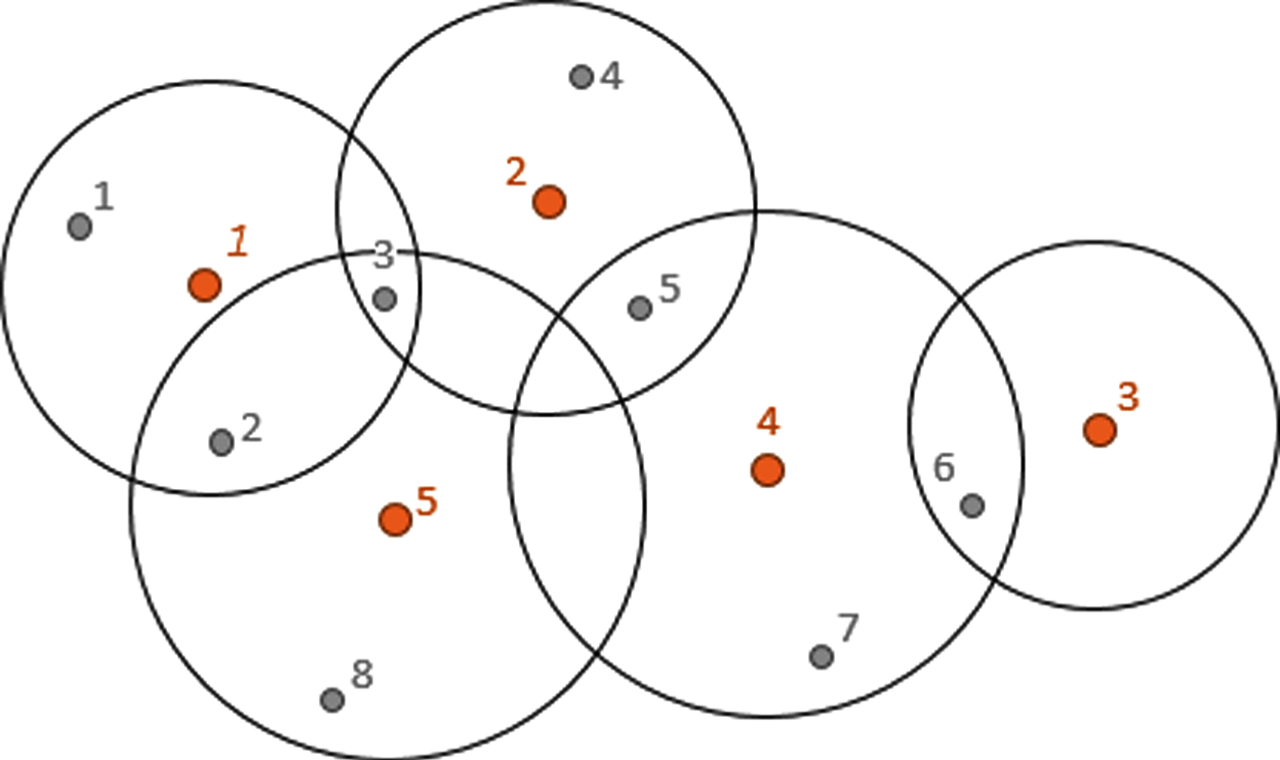
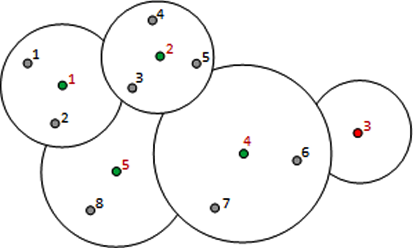
As we have noted, imprecision and uncertainty arise from the extreme situations while moving from centers to customers (see Fig. 1). Imprecision is mainly reflected in growth of inaccuracies of travel times –deviations from the average times required to deliver goods to customers in normal situations. For example, if in a normal situation it takes 20-minute to move between certain points, the expert can evaluate the movement time between the same points in the extreme situation as “about 25 minutes, ± 10 minutes”, which can be written as triangular fuzzy number (15, 25, 35) [9]. As regards the uncertainty, in extreme and uncertain environment, the possibility of movement between specific points is questioned because of lack of complete information about road conditions or because of having information about some damages on the roads. We use a possibility measure [9] to describe the feasibility of movement between points. However, due to the specifics of our problem, we consider not only the possibility of movement, but the possibility of movement in τtime. Let us assume that DP = {dp₁, dp₂, . . . , dp_p} is the set of all demand points (customers). Therefore, for each candidate center CC_j (j-th HADC), we will define DP^j–a set of the customers, for which the goods can be supplied in time τ:

Fig. 1

Facility location network.

$\begin{matrix} {DP}^{j} = {{dp}_{i} \in DP | Possibility ({\tilde{t}}_{ij} ⩽ τ) ⩾ λ}, \\ 0 ⩽ λ ⩽ 1, j = \bar{1, m}, \end{matrix}$ where ${\tilde{t}}_{ij}$ is a fuzzy movement time between demand point i = 1, …, p and candidate center j = 1, …, m ; λ is the minimal possibility level, which is defined by the emergency situation managers and by which the condition of on-time goods delivery ( ${\tilde{t}}_{ij} ⩽ τ$ ) must be satisfied (Fig. 2).

Fig. 2

Map of coverings.

The formation of expert’s input data for attributes is an important task of the centers’ selection problem. The expert e_k has to construct a binary fuzzy relation $A_{k} = {α_{ij}^{k}, i = 1, . . ., m; j = 1, . . ., n}$ - decision making matrix, elements of which are represented in q-ROFNs. Experts’ data must be aggregated in etalon decision making matrix – $A = {α_{ij}, i = 1, . . ., m; j = 1, . . ., n} .$

5 Bi-criteria model for FFLTP in extreme and uncertain environment

First, let us clarify what is a solution of our model. The solution must allocate (assign) each customer to a single candidate center, that means that this candidate center has to be opened, and the goods will be delivered from this center to the customers allocated to it. The distribution of customers to the centers should be done in such a way that the costs would be minimal and the reliability of goods delivery would be high.

In our model we make some assumptions, namely, we suppose that the model deals with distribution of uniform goods, and each customer is serviced only by one center. For the example of delivering humanitarian aid, we can assume that this aid (e.g., food or various items) is packed in homogeneous boxes - in humanitarian packages and is delivered to customers in this form. For example, one customer may need 31 boxes, another 53. We also assume that all customers must be fully serviced and, at the same time, each customer must be serviced only from one center, because in emergency situations often there is no time for coordination between the centers to plan customers’ service from multiple centers.

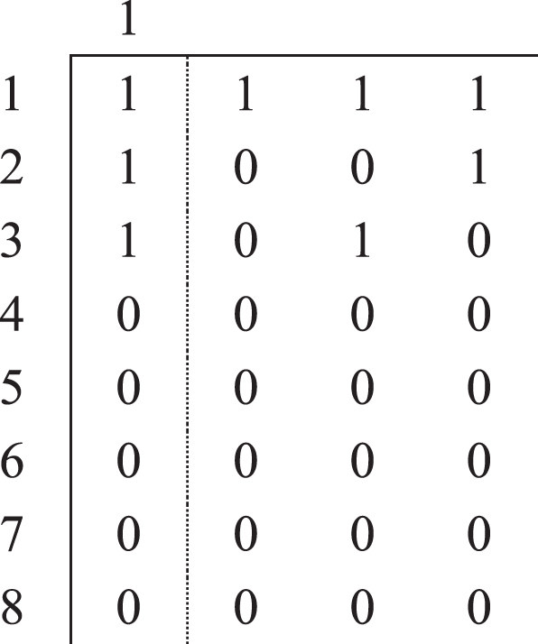
Obviously, to find optimal solutions is not a trivial task, since it requires considering a very large number of combinations –different allocations of customers to the centers. For analysis of the number of such combinations, one may look at the map of coverings, which can easily be described by so called coverings matrix A–rows of which correspond to the customers and columns of which correspond to the candidate centers (see Fig. 2’):

Fig. 2’

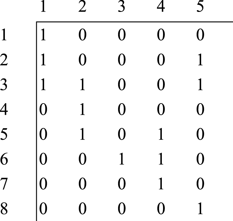
Coverings matrix A.

Fig. 3

Generated matrix A’.

Based on the map of coverings (and on the corresponding matrix), we can easily determine the number of partitionings (of customers by centers) –the number of different allocations. Our goal is to select the optimal one(s) out of these allocations. By the well-known principle of multiplication of combinatorics for the computation of variants’ numbers, the number of allocations is equal to the product of numbers of 1 s in each row (not considering customers’ demands and candidate centers capacities). In our example, the number of allocations will be 1 x 2 x 3 x 1 x 2 x 2 x 1 x 1 = 24.

Let us denote the matrix of coverings by $A = a_{ij}, a_{ij} \in {0, 1}; i = \bar{1, p}; j = \bar{1, m}$ . Then the number of partitionings elementarily can be calculated by the expression: $\prod_{i = 1}^{p} \sum_{j = 1}^{m} a_{ij} .$

In order to avoid generating all partitionings, calculating the values of objective functions and selecting Pareto optimal solutions out of them, we propose an approach, which allows us to find Pareto optimal solutions without performing exhaustive search.

Now we present the model in more formal way. The objective data for the model is:

p –Number of demand points (customers);

DP = {dp_i}–Set of demand points, $i = \bar{1, p};$

d_i–Demand of i-th demand point, $i = \bar{1, p};$

m–Number of candidate centers (HADCs);

CC = {cc_j} –Set of candidates (potential) centers, $j = \bar{1, m};$

C_j–Capacity of j-th center, $j = \bar{1, m};$

P_j –Cost of opening j-th center;

μ_ij –Cost of transporting (d_igoods) from j-th center to i-th demand point;

τ –Maximum allowed time to deliver goods to demand points;

The subjective (expert) data for the model is:

${DP}^{j} = {{dp}_{i} \in DP | Possibility ({\tilde{t}}_{ij} ⩽ τ) ⩾ λ}$ –Map of coverings, which is based on expert evaluations and satisfies the condition ${\tilde{t}}_{ij} ⩽ τ$ , with λ minimal possibility level, $j = \bar{1, m};$

γ = {γ_j} , γ_j ∈ [0, 1]–Centers’ selection indexes, $j = \bar{1, m}$ , defined in Section III.

Variables:

r_j ∈ {0 ; 1} :1- if j-th HADC is opened, else 0;

x_ij ∈ {0 ; 1} :1- if i-th customer’s d_i demand is fully satisfied by j-th HADC, else 0 (when i-th customer is not serviced from j-th HADC);

It is obvious, that $r_{j} = \lor_{i = 1}^{p} x_{ij} (= max_{i = 1, p} x_{ij})$ .

Based on above judgment we create the following bi-criteria problem of partitioning, where the first objective function is of transportation type and the second objective function is of facility location type.

Objective functions: $f_{1} = \sum_{j = 1}^{m} P_{j} r_{j} + \sum_{i = 1}^{p} \sum_{j = 1}^{m} μ_{ij} x_{ij} \to min,$ (3) $f_{2} = \lor_{j = 1}^{m} (1 - γ_{j}) r_{j} \to min,$ (4)

Constraints:

For the capacities of the HADCs (a constraint of transportation type): $\sum_{i = 1}^{m} d_{i} x_{ij} ⩽ C_{j}, j = \bar{1, n}$

For the selection indexes of the HADCs (a constraint of facility location type): $γ_{j} \in [0, 1] .$ (5)

Here $x_{ij} \in {0; 1}; r_{j} \in {0; 1} .$ (6)

For single customer being fully satisfied from single HADC: $\sum_{i = 1}^{m} x_{ij} = 1, i = \bar{1, p},$ (7) where ∧ and ∨ represent min and max operators, respectively; criterion (3) is a minimization of goods transportation and HADCs opening total costs and criterion (4) is a minimization of HADCs’ “not selecting” index, which can be changed by the criterion maximization of HADCs’ selection index: $f_{2}^{*} = \land_{l j = 1 r_{j} \neq 0}^{m} γ_{j} r_{j} \to max .$

Finally, for the HADCs location and goods transportation problem a bi-criteria Boolean problem (3)-(7) is constructed.

6 Solution of the bi-criteria partitioning problem

Our approach for solving the constructed bi-criteria Boolean problem (3)-(7) consists of two stages. In the first stage, based on the covering’s matrix A, we generate a new matrix A′, columns of which allow us to find all possible partitionings of the customers relative the centers. Some constraints are also taken into consideration while generating the matrix A′. In the second stage, using the matrixA′ and the exact algorithm constructed by the authors of this work we find the partitionings –allocations of the demand points to the potential centers - which correspond to the Pareto-optimal solutions ([10]). Let us discuss each of the stages in details:

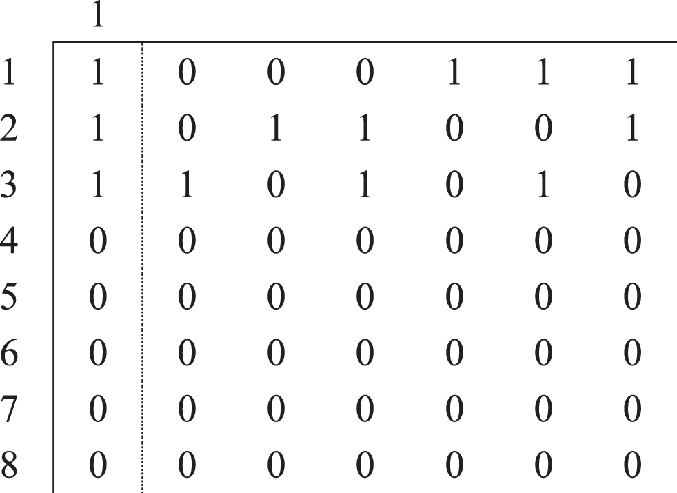
Stage I: Based on matrix A of covering, we generate a new matrix $A^{'} = a_{ij}^{'}, a_{ij}^{'} \in {0, 1}, i = \bar{1, m}; l = \bar{1, s}$ , columns of which allow us to find all partitionings of customers (demand points). This means that each and every customer must be covered by a single center, so the matrix Amust contain exactly one 1 in each row. Therefore, each customer is allocated to the single center despite the fact that the same customer could be covered by other centers in the τtime.

The principle of generating the columns of the matrix A′is as follows: based on the matrix A, we generate all possible columns, which can serve as a column for partitioning matrix. This means that any of 1s in the column of the matrix A can become 0, maybe several of 1 s, but not all of them together (having this kind of columns in the matrix doesn’t make any sense). In the case of the example which was presented above, the first column will generate following columns:

As we can see in generated columns zeros are unchanged in the rows 4 - 8, which is logical since the service center (HADC) corresponding to the first column can’t cover these customers (in τ time).

While generating the columns of matrix A′ we can additionally take into consideration the following factor: if the matrix A had single 1 in some row, it can’t become 0. Therefore, in generated columns 1 s must be unchanged in the corresponding row. To say the same in simpler words, if a specific customer is covered only by one HADC, this customer will be covered by this single HADC in every partition. In the example given above, we have single 1 in the first row (in the first column), thus the first column of the matrix A will not generate the columns which were listed above, but only following three columns (not including itself):

Finally, the matrix Agives us the following A′matrix:

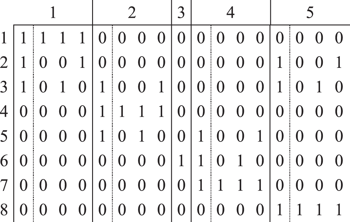
The columns of the matrix A′are grouped by the columns of the matrix A.

While generating the columns of the matrix A′ we can also take into consideration C_j ( $j = \bar{1, n}$ ) capacities of the HADCs. If for any specific column q, sum of the d_i demands of the customers corresponding to the 1 s in this column, exceeds the C_j capacity of the HADC ( $\sum_{i = 1}^{m} a_{ij}^{'} d_{i} > C_{j}$ ), which is the “parent” for the q-th column, we must remove this column from the matrix A′, since this column can’t exist in any solution.

Let s be the number of columns (after filtration) of the matrix A′ and s_j be the number of columns in j-th column of the matrix A′. Obviously, $s = \sum_{j = 1}^{n} s_{j}$ .

Stage II: We perform conversion of the variables, constraints and objective functions of the initial problem to the terms of the matrix A′ and execute our exact algorithm of bicriteria partitioning. As a result, we find the partitionings –allocations of the customers to the HADCs –which will be the Pareto optimal solutions.

Our algorithm of bi-criteria partitioning is based on the extended algorithm [20] of Dancing Links technique and DLX algorithm proposed by D. Knuth [16]. Also, the algorithm implements the epsilon-constraint method for multi-criteria optimization problems [4 , 10]. Due to dynamic programming techniques the algorithm effectively uses RAM and, therefore, is characterized with high performance, it can also run-in parallel mode and handle problems of large dimensions. The most important point is that the algorithm finds exact Pareto front –all Pareto optimal solutions. The algorithm can solve in several seconds the problems having approximately 100×1000 dimensions. These dimensions are sufficient for dealing with absolutely most real-life problems, presented in this work.

Let us formulate the bi-criteria partitioning problem in terms of the matrix A′. Let’s introduce a Boolean variable z_l ∈ {0 ; 1} , z = (z₁, z₁, . . . , z_s) z_l = 1–if the l-th column of the matrix A′is included in the solution, else 0, $l = \bar{1, s}$ .

Objective functions will have the form: $f_{1}^{'} = \sum_{l = 1}^{s} (P_{l}^{'} + μ_{l}^{'}) z_{l} \to min,$ (8) $f_{2}^{'} = \lor_{l = 1}^{s} (1 - γ_{l}^{'} {) z}_{l} \to min,$ (9)

With partitioning constraints: $A^{'} z^{T} = (1, 1, . . ., 1),$ (10) where: $\begin{matrix} P_{l}^{'} = P_{k}, μ_{l}^{'} = \sum_{i = 1}^{m} μ_{ik} a_{il}^{'}, γ_{l}^{'} = γ_{k}; \\ l = 1 + \sum_{j = 0}^{k - 1} s_{j}, . . ., \sum_{j = 0}^{k} s_{j}; s_{0} \equiv 0; k = 1, . . ., n . \end{matrix}$

Indeed, l takes values from 1 to s ( $s = \sum_{j = 1}^{n} s_{j}$ ), therefore, ltakes the values from the following intervals (corresponding to the column groups of the matrix A′): $\begin{matrix} [1, s_{1}], [1 + s_{1}, s_{1} + s_{2}], [1 + s_{1} + s_{2}, s_{1} + s_{2} \\ + s_{3}], . . ., [1 + \sum_{j = 1}^{n - 1} s_{j}, \sum_{j = 1}^{n} s_{j} = s] . \end{matrix}$

In the k-th group $P_{l}^{'} = P_{k}$ is fixed. The same is true for $γ_{l}^{'}$ ( $γ_{l}^{'} = γ_{k}$ ). As regards the second addend of the objective function (8) –transportation costs –it depends on the 1 s, which will stay in the column of k-th group of the matrix A′from the k-th column of the initial matrix A.

As for the constraints, the HADCs capacity constraints are already taken into consideration during the generating process of the matrix A′and solving the partitioning problem for the rows and columns of the matrix A′ automatically means satisfying the second constraint –any customer must be fully satisfied from the single HADC.

If we execute our exact algorithm on the matrix A′to solve the problem (8) - (10), we find the partitionings, which correspond to the Pareto optimal solutions. Each of them will have the form of a matrix, rows of which corresponds to the customers and columns represent the subset of the columns of the matrix A′.

If we analyze the matrixA′, we can notice, that the following proposition is true (without proof):

Proposition 1. Each solution (Pareto optimal partitioning) can contain no more than one column from each column group of the matrix A′.

Indeed, in each column group contains all possible coverings of customers by specific HADC (we mean the customers, which can be covered by the HADC in τ time). While searching the minimal partitioning, if we find out that the specific HADC covers for example pnumber of customers, from the column group corresponding to this HADC, the algorithm will always choose the column which contains pnumber of 1 s and will not choose the separate columns (from the same column group), union of which is identical of the above mentioned column (containing pnumber of 1 s). Note: the columns with intersecting 1 s can’t be included in the partitioning solution.

As a summary, we can note that our approach for solving (8)-(10) bi-criteria problem is better than exhaustive search approach, because based on the matrix A′it generates only the admissible (satisfying the constraints) and interesting (not worse that already identified in previous steps of the algorithm) partitionings. Main results’ support software is designed, including authors’ algorithm [20] based on D. Knuth’s “DLX” algorithm.

7 Model illustration. Numerical example

To illustrate the model, we have described, and the approach to its solution, let us consider a small dimensional example. Suppose we have p = 8 demand points and m = 5 potential locations where humanitarian aid distribution centers can be opened (Fig. 2). The data of moving fuzzy times between demand points and candidate centers are omitted here, because Fig. 2 defines Map of coverings for some time τ. We use only five main attributes (n = 5) defined above by short names: x₁ =”Accessibility”, x₂ =”Security”, x₃ =“Connectivity to multimodal transport”, x₄ =”Costs”, x₅ =”Proximity to customers”. The fourth attribute is cost type and the others are benefit types. As mentioned above, cost type evaluation data must be transformed in the benefit forms.

Suppose the experts generated the attributes weights as values of overall importance based on the consensus: w₁ = 0.25 ; w₂ = 0.15 ; w₃ = 0.25 ; w₄ = 0.20 ; w₅ = 0.15. Let three experts have equal ratings {ω_j = 1/3}, and assume that each expert ex_k (k = 1, 2, 3) presented the q-rung orthopair fuzzy ratings $r_{ij}^{k}$ for each candidate center cc_i, (i = 1, . . . , 5), with respect to each attribute x_i, (i = 1, . . . , 5).

Using formula (1) experts’ evaluations are aggregated in decision making matrix {α_ij} (Table 4).

Table 1
Appraisal matrix by expert-1

x ₁ x ₂ x ₃ x ₄ x ₅

cc ₁ (0.7, 0.5) (0.8, 0.3) (0.7, 0.4) (0.7, 0.4) (0.8, 0.4)

cc ₂ (0.6, 0.5) (0.7, 0.4) (0.4, 0.6) (0.8, 0.4) (0.7, 0.4)

cc ₃ (0.7, 0.5) (0.9, 0.5) (0.9, 0.7) (0.7, 0.4) (0.8, 0.5)

cc ₄ (0.6, 0.5) (0.8, 0.4) (0.8, 0.5) (0.9, 0.5) (0.8, 0.5)

cc ₅ (0.8, 0.6) (0.7, 0.4) (0.9, 0.5) (0.7, 0.4) (0.8, 0.6)

	x ₁	x ₂	x ₃	x ₄	x ₅
cc ₁	(0.7, 0.5)	(0.8, 0.3)	(0.7, 0.4)	(0.7, 0.4)	(0.8, 0.4)
cc ₂	(0.6, 0.5)	(0.7, 0.4)	(0.4, 0.6)	(0.8, 0.4)	(0.7, 0.4)
cc ₃	(0.7, 0.5)	(0.9, 0.5)	(0.9, 0.7)	(0.7, 0.4)	(0.8, 0.5)
cc ₄	(0.6, 0.5)	(0.8, 0.4)	(0.8, 0.5)	(0.9, 0.5)	(0.8, 0.5)
cc ₅	(0.8, 0.6)	(0.7, 0.4)	(0.9, 0.5)	(0.7, 0.4)	(0.8, 0.6)

Table 2

Appraisal matrix by expert-2

	x ₁	x ₂	x ₃	x ₄	x ₅
cc ₁	(0.7, 0.5)	(0.8, 0.4)	(0.6, 0.3)	(0.6, 0.3)	(0.7, 0.4)
cc ₂	(0.6, 0.5)	(0.7, 0.3)	(0.7, 0.4)	(0.9, 0.4)	(0.8, 0.4)
cc ₃	(0.8, 0.5)	(0.9, 0.5)	(0.6, 0.4)	(0.8, 0.4)	(0.6, 0.2)
cc ₄	(0.6, 0.4)	(0.8, 0.3)	(0.9, 0.6)	(0.7, 0.3)	(0.6, 0.2)
cc ₅	(0.9, 0.7)	(0.7, 0.4)	(0.9, 0.4)	(0.7, 0.3)	(0.9, 0.6)

Table 3

Appraisal matrix by expert-3

	x ₁	x ₂	x ₃	x ₄	x ₅
cc ₁	(0.7, 0.4)	(0.8, 0.3)	(0.7, 0.5)	(0.7, 0.4)	(0.9, 0.5)
cc ₂	(0.6, 0.5)	(0.7, 0.4)	(0.5, 0.3)	(0.7, 0.2)	(0.6, 0.3)
cc ₃	(0.6, 0.2)	(0.9, 0.6)	(0.7, 0.5)	(0.7, 0.3)	(0.6, 0.3)
cc ₄	(0.8, 0.4)	(0.9, 0.4)	(0.8, 0.5)	(0.8, 0.5)	(0.8, 0.3)
cc ₅	(0.9, 0.7)	(0.6, 0.3)	(0.9, 0.5)	(0.9, 0.6)	(0.7, 0.4)

Table 4

Accumulated q = q₀ = 4-rung orthopair fuzzy decision matrix {α_ij}

	x ₁	x ₂	x ₃	x ₄	x ₅
cc ₁	(0.70,0.46)	(0.80,0.33)	(0.67,0.39)	(0.67,0.36)	(0.83,0.43)
cc ₂	(0.60,0.50)	(0.70,0.36)	(0.58,0.42)	(0.83,0.32)	(0.72,0.36)
cc ₃	(0.72,0.37)	(0.90,0.53)	(0.79,0.52)	(0.74,0.36)	(0.70,0.31)
cc ₄	(0.70,0.43)	(0.84,0.36)	(0.84,0.53)	(0.83,0.42)	(0.76,0.31)
cc ₅	(0.88,0.66)	(0.67,0.36)	(0.90,0.46)	(0.80,0.42)	(0.83,0.52)

After application of the steps of Fuzzy TOPSIS algorithm for evaluation of candidate centers selection indexes the following estimation are obtained (calculating results of Section 3 are omitted because of large number of calculations): γ = {γ_j} = {0.28, 0.56, 0.14, 0.30, 0.33}.

Below is given the specific numerical data relevant to the optimization problem.

Demand points requirements vector: D = {d_i} = {120, 215, 145, 110, 181, 210, 172, 168}; Candidate centers capacities vector: C = {C_j} = {460, 450, 400, 470, 500};

Candidate centers opening costs vector: P = {P_j} = {1100, 1000, 800, 1200, 900} ;

Transportation costs matrix M = ||μ_ij||:

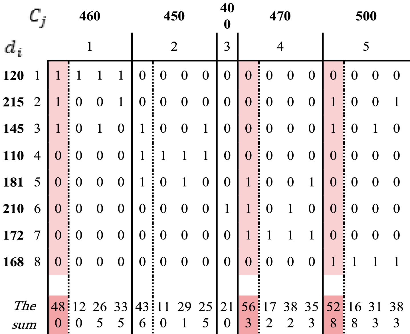
To solve the problem, in accordance with Phase I of the above considered methodology, let us generate the matrix A’ based on the matrix A of coverings and remove from it those columns that violate the capacity constraints of the centers (Fig. 3, columns to be removed are marked with a different color).

Finally, we obtain $A^{'} = | | a_{il}^{'} | |, a_{il}^{'} \in {0; 1},$ $i = \bar{1, 8}; l = \bar{1, 14};$ i.e., 8×14 dimensional matrix (the values of the objective functions are written in the last two lines, (Fig. 4):

Fig. 4

Generated matrix A’ with objectives.

According to the Stage II of our approach, let us apply on matrix A′ the exact bicriteria partitioning algorithm [20, 21] which is worked out by the authors of this paper. As a result, we obtain two partitionings which correspond to the optimal solutions:

Solution 1: CC₁₃, CC₂₁, CC₃₁, CC₄₁, CC₅₁

Total cost: 8575; Total selection ranking index: 0.36 (= 1 - 0.64);

Solution 2: CC₁₃, CC₂₁, CC₄₂, CC₅₁

Total cost: 8882; Total selection ranking index: 0.56 (= 1 –0.44);

Solution 2: A geometric interpretation see in Fig. 5.

Fig. 5

Geometric interpretation of partitioning.

As for interpreting solutions based on matrix A′ and translating into the initial problem terms, it is a simple task, since the columns (cc_ij) in the solution give information about which centers (cc_i) should be opened as well as which customer (demand point) should belong to which center (for this column in rows of such as demand points ‘1’ are inserted). For example, if we consider the second solution, it turns out that the third potential center should not open and the assignments should be as follows (see Fig. 4. The centers that should open are reddened).

Given the essence of Pareto-optimality, as we can see, the first solution has the better value of total cost than the second. However, the second solution has a higher reliability because the total selection ranking index of the centers is better.

8 Comparative analysis

The new model of FFLTP presented in this article is distinguished by the fact that by the new objective function we minimize the risks of opening of HADCs. The coefficients of the new objective function are the selection indices of HADCs. To evaluate the latter, we used the distinctive and popular heuristic method of ranking alternatives in decision-making models - TOPSIS. Of course, other methods (VIKOR (an acronym in Serbian for multicriteria optimization and compromise solution), AHP (Analytic Hierarchy Process), TODIM (an acronym in Portuguese for interactive multi-criteria decision making), etc.) or their combinations can also be used, and this represents the degree of freedom of approach we offer. It all depends on the preferences of the user. Why did we use TOPSIS and not another approach? The TOPSIS approach was chosen for one simple reason. From the heuristic approaches developed in recent years that identify alternatives in decision-making models, the TOPSIS approach is characterized by stable, sustainable results and a fairly simple execution scheme. Besides, it is a practical and useful technique for ranking and selection from a number of externally determined alternatives through distance measures.

When the optimization model is already built as a bi-criteria Boolean optimization problem, the next step is to look for optimal ways to solve it. Since due to the specifics of the problem we are not dealing with large dimensions of the problem, therefore exact methods of solving have no alternative. The main finding of this paper is that the constructed model can be reduced by simple transformations to the problem of bicriteria partitioning, for which we have developed an epsilon-constraint approach for the identification of Pareto solutions [20, 21]. As a result, there are several well-known algorithmic methods for solving each scaled problem [7, 11]. However, all these algorithms would give the same result overall - the Pareto solution front. We have chosen a method based on D. Knut algorithm [16], the parallelized variation of which has been developed in our early works [20, 21].

From the above reasoning, we see that the problem-solving scheme presented in this article is competitive with other methods since, on the one hand, due to the first paragraph of the current section, we are free in choosing a heuristic approach to the evaluation of selection indices and it depends on the user, and on the other hand, due to the second paragraph of this section, only exact approaches are expedient and we have chosen a well-proven fast algorithm for us. However, using another exact algorithm would give us the same Pareto solutions.

9 Conclusions

A q-rung orthopair fuzzy TOPSIS approach for formation and representation of expert’s knowledge on the parameters of emergency service facility location planning is developed. In this approach, we propose a score function-based comparison method to identify the q-rung orthopair fuzzy positive ideal solution and the q-rung orthopair fuzzy negative ideal solution. Based on the constructed fuzzy TOPSIS aggregation a new innovative objective function is formulated. Constructed criterion maximizes selected service centers’ index and reduces HADCs opening risks. Bi-objective facility location-selection/transportation partitioning problem is constructed. We constructed innovative two stage approach for solving the constructed bi-criteria partitioning problem. In the first stage we create algorithm, based on which the coverings matrix is transformed into a new matrix. Columns of transformed matrix allow us to find all possible partitionings of the HADCs with the service centers. In the second stage, using the transformed matrix and our exact algorithm [18, 19] we find the partitionings –allocations of the HADCs to the centers which correspond to the Pareto-optimal solutions. For illustration of constructed model, a numerical example is considered. From the practical point of view, more detailed and deep constraints will be considered in our future FFLTP’s models.

Footnotes

Acknowledgments

This work was supported by Shota Rustaveli National Science Foundation of Georgia (SRNSFG) [FR-18-466].

References

Abounacer

, Rekik

and Renaud

, An Exact Solution Approach for Multi-objective Location–transportation Problem for Disaster Response, Computers & Operations Research 41 (2014), 83–93.

Aikens

C.H.

, Facility location models for distribution planning, European Journal of Operational Research 22 (1985), 263–279.

Atanassov

, Intuitionistic fuzzy sets, Fuzzy Sets and Systems 20 (1986), 87–96.

Bérubé

J.F.

, Gendreau

and Potvin

J.Y.

, An Exact Epsilon-constraint Method for Bi-objective Combinatorial Optimization Problems: Application to the Traveling Salesman Problem with Profits, European Journal of Operational Research 194(1) (2009), 39–50.

Caunhye

A.M.

, Nie

and Pokharel

, Optimization model in emergency logistics: A literature review, Socio-Economic Planning Sciences 46 (2012), 4–13.

Chu

T.C.

, Facility location selection using fuzzy TOPSIS under group decisions, International Journal of Uncertainty Fuzziness and Knowledge-Based Systems 10(6) (2002), 687–701.

Christofides

, Graph theory, an algorithmic approach. Orlando, FL: Academic Press. (1975).

Daskin

M.S.

, Network and Discrete Location Models, Algorithms, and Applications, John Wiley & Sons 1-28 (2013), 362–479.

Dubois

and Prade

, Possibility Theory: An Approach to Computerized Processing of Uncertainty, New-York: Plenum Press, (1988), 1–72.

10.

Ehrgott

, Multicriteria optimization, Springer-Verlag Berlin, Heidelber, (2005), 1–20, 65-80, 78-111, 197-220.

11.

Fisher

M.L.

and Kedia

, Optimal solution of set covering/partitioning problems using dual heuristics, Management Science 36 (1990), 674–688.

12.

Guo

and Qi

, Modeling and Simulation of Emergency Service Facilities Location Problem Under Fuzzy Environment, The Open Mechanical Engineering Journal 8 (2014), 48–52.

13.

Haddow

G.D.

, Bullock

J.A.

and Coppola

D.P.

, Introduction to Emergency Management. USA: Butterworth-Heinemann. (2008).

14.

Zhang

, Dong

, Xiao

, Chiclana

and Herrera-Viedma

, Personalized individual semantics-based approach for linguistic failure modes and effects analysis with incomplete preference information, IISE Transactions 52(11) (2020), 1275–1296.

15.

Hwang

C.L.

and Yoon

, Multiple attribute decision making: methods and applications. Berlin, Heidelberg: Verlag, (1981), 58–191.

16.

Knuth

D.E.

, Dancing Links. Millennial Perspectives in Computer Science, Palgrave, Houndmills, Basingstoke, Hampshire, (2000), 187–214.

17.

, Liu

and Chen

, Selection of Logistics Center Location. Using Axiomatic Fuzzy Set and TOPSIS Methodology in Logistics Management, Expert Systems with Applications 38 (2011), 7901–7908.

18.

Liu

, Zhang

, Wu

and Dong

, Ranking range based approach to MADM under incomplete context and its application in venture investment evaluation, Technological and Economic Development of Economy 25(5) (2019), 877–899.

19.

Sirbiladze

, Fuzzy Identification Problems for Continuous Extremal Fuzzy Dynamic System, Fuzzy Optimization and Decision Making 9 (2011), 233–274.

20.

Sirbiladze

, Sikharulidze

, Ghvaberidze

and Matsaberidze

, Fuzzy-probabilistic Aggregations in the Discrete Covering Problem, International Journal of General Systems 40(2) (2011), 169–196.

21.

Sirbiladze

, Ghvaberidze

and Matsaberidze

, Bicriteria Fuzzy Vehicle Routing Problem for Extreme Environment, Bulletin of the Georgian National Academy of Sciences 8(2) (2014), 41–48.

22.

Sirbiladze

, Ghvaberidze

and Matsaberidze

, A New Fuzzy Model of the Vehicle Routing Problem for Extreme Conditions, Bulletin of the Georgian National Academy of Sciences 9(2) (2015), 46–53.

23.

Sirbiladze

, Ghvaberidze

, Matsaberidze

and Sikharulidze

, Multi-Objective Emergency Service Facility Location Problem Based on Fuzzy TOPSIS, Bulletin of the Georgian National Academy of Sciences 11(1) (2017), 23–30.

24.

Sirbiladze

, Ghvaberidze

and Matsaberidze

, Fuzzy Aggregation Operators Approach in Location/Transportation Problem, Bulletin of the Georgian National Academy of Sciences 12(3) (2018), 32–33.

25.

Sirbiladze

, Ghvaberidze

, Matsakberidze

and Midodashvili

, New fuzzy approach to facility location problem for extreme environment, Journal of Intelligent & Fuzzy Systems 37(6) (2019), 7883–7893.

26.

Verdegay

J.L.

, Progress on Fuzzy Mathematical Programming: A Personal Perspective, Fuzzy Sets and Systems 281 (2015), 219–226.

27.

Yager

R.R.

, Pythagorean membership grades in multi-criteria decision making, IEEE Transactions on Fuzzy Systems 22(4) (2014), 958–965.

28.

Yager

R.R.

, Generalized Orthopair Fuzzy Sets, IEEE Transactions on Fuzzy Systems 25(5) (2017), 1222–1230.

29.

Yager

R.R.

and Alajlan

, Approximate Reasoning with Generalized Orthopair Fuzzy Sets, Information Fusion 38 (2017), 65–73.

30.

Yong

, Plant location selection based on fuzzy TOPSIS, International Journal of Advanced Manufacturing Technology 28 (2006), 839–844.

31.

Zadeh

L.A.

, Fuzzy sets, Information and Control 8 (1965), 338–353.

32.

Zokaee

, Bozorgi-Amiri

and Sadjadi

S.J.

, A robust optimization model for humanitarian relief chain design under uncertainty, Applied Mathematical Modelling 40 (2016), 7996–8016.