Shadow detection of soil image based on density peak clustering and histogram fitting

Abstract

Shadow detection is a significant preprocessing work that soil type is classified with machine vision. Thus, Density peak clustering based on histogram fitting(DPCHF) is proposed to segment soil image shadows. First, its clustering centers are adaptively obtained by constructing a new parameterless density formula and decision value measure. Then the Fourier series are drawn into it to approximate the gray histogram and a part of gray-levels are allocated by valley points of the histogram fitting curve. Finally, an optimization model is established to optimize the threshold of detecting the shadow in the soil image, and the remaining gray-levels are clustered by the threshold. The simulation results show that DPCHF is better than the contrast algorithm. The average brightness standard deviations of the shadow and non-shadow are respectively 20.9348 and 20.3081 with DPCHF. It can realize the adaptive shadow detection of soil images and there is not the “domino” error propagation in it.

Keywords

Shadow detection density peak clustering soil image machine vision

1 Introduction

Due to the influence of uneven soil surface, cavity and photography angle, there are shadows in the soil images that are collected by machine vision. For identifying soil species, usually the soil images are cut for some sub-images that their size is standard and a sub-image is full soil. If there are many dark shadows in some of soil sub-images, the learning machine that is trained by the soil sub-images maybe mistakenly identify soil species of soil image. The principal reason is that shadows hide the inherent characteristics of the soil and mislead the learning machine. And it will reduce the accuracy of soil species identification with machine vision. In order to highlight the soil characteristics of the sub-image, it is avoided that more shadow areas are cut into soil sub-image for identification of soil species by machine vision. Thus, Shadow detection is a necessary preprocessing work for eliminating its influence.

The shadow detection of soil images is a segmentation work. Density peaks clustering (DPC) [1] is an efficient clustering algorithm, which is widely used in image segmentation. Predecessors have made many effective improvements on DPC algorithm [2 –10] and it include two aspects. One is to solve the problem that DPC is strongly dependent on density kernel and empirical parameter cutoff distance d_c [11 –15]. For example, Zhen [11] introduced information entropy to improve the cutoff distance d_c, and Wang [12] used Gini impurity to find the best cut-off distance d_c, Hou [13] raised a new density kernel and normalized the density to reduce the dependence of DPC on the cutoff distance d_c, and Jiang [14] proposed a method to calculate d_c based on the Gini coefficient, and Chun [15] put forward an improved density peaks clustering algorithm based on the layered k-nearest neighbors and subcluster merging. The other is to solve the problem that DPC needs to select the cluster center manually, and a series of algorithms to obtain the cluster center automatically are proposed [16 –20]. For example, Liang [16] came up with an improved 3DC algorithm to obtain clustering center adaptively, and Liu [17] proposed adaptive clustering algorithm which introduced the idea of K-nearest neighbors (named as ADPC-KNN), and Zeng [18] constructed center decision metric CDM_i to obtain automatically cluster centers.

However, the above studies can not solved the problem of “domino” error propagation. That is a point allocation error leads to joint errors of other points and it is caused by the DPC algorithm because there is the same allocation strategy for all data in the DPC algorithm. Therefore, the DPC algorithm needs further research and improvement for the shadow detection of soil images.

The rest of this paper is organized as follows. Section 2 reviews the original DPC algorithm. The density peak clustering based on histogram fitting is introduced in Section 3. Experimental results are shown in section 4 and Section 5 is the conclusion of this paper.

2 Density peaks clustering(DPC)

The density peak clustering algorithm defines local density ρ_i and relative distance δ_i for each data point x_i in the dataset. The local density ρ_i is

ρ_{i} = \sum_{j = 1, j \neq i}^{N} χ (d_{ij} - d_{c})

(1)

Where d_ij expresses the Euclidean distance from x_i to x_j, d_c denotes the cutoff distance. If d_ij - d_c < 0, then χ (d_ij - d_c) = 1, otherwise χ (d_ij - d_c) = 0.

The relative distance δ_i is

δ_{i} = {\begin{matrix} min_{j} (d_{ij}) \begin{matrix}  \end{matrix} if \exists j ρ_{j} > ρ_{i} \\ max_{j \neq i} (δ_{j}) \begin{matrix}  \end{matrix} \begin{matrix}  \end{matrix} otherwise \end{matrix}

(2)

The original DPC algorithm manually selects the points with relatively large ρ and δ values as the clustering center. Then arrange the density of each remaining point in descending order to assign each point to the nearest neighbor whose density is larger than itself until all of the remaining points belong to their cluster centers.

3 Density peak clustering based on histogram fitting(DPCHF)

There are three steps in the density peak clustering algorithm based on histogram fitting(DPCHF). It includes constructing a new nonparametric density formula for an adaptive decision value measure. Then introducing the Fourier series to approximate automatically the gray histogram and allocate a part of the gray-level by valley points of the histogram fitting curve. Finally, establishing an optimization model to search for the shadow detection threshold of the soil image and assign the remaining gray-level to complete the shadow segmentation of soil images. The flowchart of the DPCHF algorithm is shown in Fig. 1.

Fig. 1

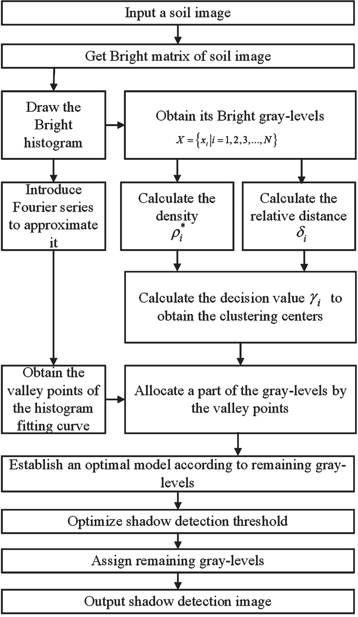
Flowchart of DPCHF algorithm.

3.1 Obtaining adaptively the clustering centers

3.1.1 Reconstructing density measure

The one-dimensional histogram of the Bright matrix of soil image is counted, and the gray-level (in ascending order) within [min(Bright) , max(Bright)] range from data set X = { x_i|i = 1, 2, 3, . . . , N }

Bright (i, j) = \frac{R (i, j) + G (i, j) + B (i, j)}{3}

(3)

where R (i, j), G (i, j) and B (i, j) represent the pixel gray values of the i-th row and j-th column of the three RGB channels of the image respectively.

The density $ρ_{i}^{*}$ of data point x_i is reconstructed as

ρ_{i}^{*} = \sqrt[3]{\sum_{j = 1, j \neq i}^{N} (\frac{π}{2} - arctan (d_{ij})) \cdot fre q_{j}}

(4)

Where d_ij denotes the Euclidean distance from point x_i to point x_j, freq_j is the number of gray values equal to x_j in the Bright matrix, expressed as the frequency of x_j points.

3.1.2 Obtaining adaptively the clustering centers

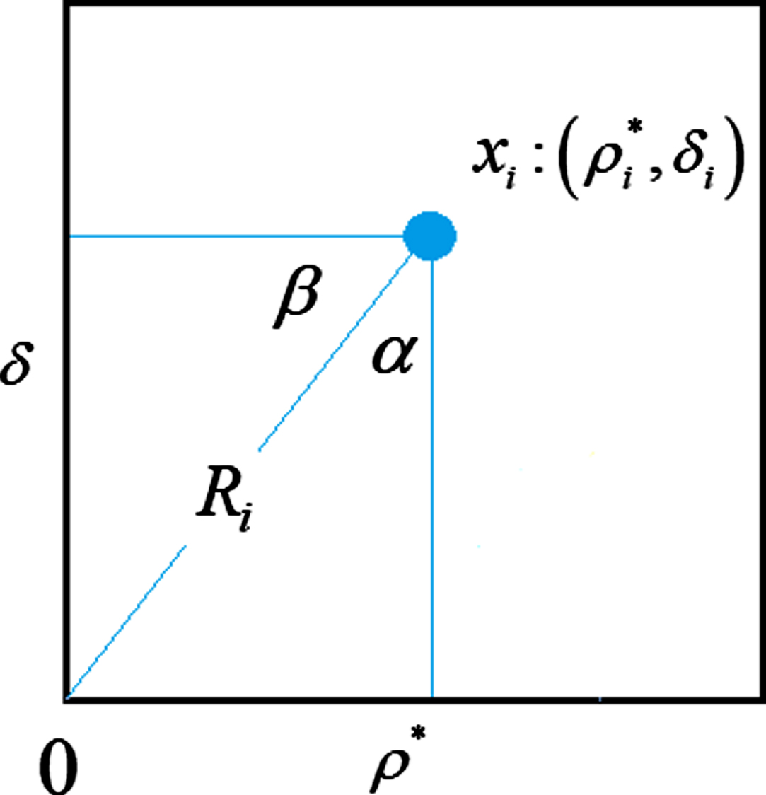
The clustering centers of DPC have the characteristics of high local density ρ_i and large relative distance δ_i. And it defined a decision value γ_i to describe the local density ρ_i and relative distance δ_i. That is, the greater ρ_i and δ_i, the greater the value of γ_i. Inspired by its idea, the decision value γ_i is reconstructed with the density $ρ_{i}^{*}$ . The x_i points with larger γ_i are selected as the clustering centers.

As shown in Fig. 2, the decision value γ_i should be redefined as

Fig. 2

$(ρ_{i}^{*}, δ_{i})$ diagram of gray-level x_i.

$γ_{i} = {\begin{matrix} φ (\cos α_{i}, cos β_{i}) \cdot ρ_{i}^{*} \cdot δ_{i}, & \cos α_{i} \neq cos β_{i} \\ ρ_{i}^{*} \cdot δ_{i}, & otherwise \end{matrix}$ (5) $φ (\cos α_{i}, cos β_{i}) = {\begin{matrix} ρ_{i}^{*} / - δ_{i}, & \cos α_{i} > cos β_{i} \\ δ_{i} / - ρ_{i}^{*}, & \cos α_{i} < cos β_{i} \end{matrix}$ (6)α denotes the angle between line R_i and the vertical line from point $(ρ_{i}^{*}, δ_{i})$ to axis ρ*, and β is the angle between line R_i and the horizontal line from point $(ρ_{i}^{*}, δ_{i})$ to axis δ.

γ_i is sorted in descending order. And the two x_i points with the two largest γ_i are chosen as the cluster centers of shadow and non-shadow because shadow detection is a typical binary classification problem. The smaller x_i in the two cluster centers is the peak point of the shadow region, which is expressed as P_left. The other matches the peak point of the non-shadow area, marked as P_right.

3.1.3 Obtaining adaptively the clustering center algorithm

Based on the above algorithm ideas, an algorithm of Obtaining adaptively the clustering centers is as Algorithm 1.

Algorithm 1 Obtaining adaptively clustering center

Require:

A soil image.

Ensure:

Shadow region peak P_left and non shadow region peak P_right.

1: The Bright of each pixel of the soil image is calculated with Eqs. (3) to form the Bright matrix A.

2: Count up a one-dimensional histogram of the Bright matrix A.

3: The Bright gray-level that frequencies are not equal to 0 are selected in the Bright histogram and are sorted in descending order to form gray-level $X = {x_{i} | i = 1, 2, 3, . . ., N}) . ∥ 4 : Calculatethedensity (ρ_{i}^{*}$ with Eqs. (4).

5: Calculate the δ_i with Eqs. (2).

6: The decision value γ_i is calculated with Eqs. (5).

7: Arrange γ_i in descending order, and the two x_i points with the two largest γ_i are selected. Set P_left equal to x_i with smaller value and P_right equal to the other.

3.2 Clustering based on histogram fitting curve

The original DPC algorithm assigned data point x_i to its nearest neighbor whose distance δ_i from x_i to the nearest neighbor is minimum, and the local density of the nearest neighbor is higher than the local density of data point x_i. It may cause the misclassification of data points to affect the segmentation effect. In order to avert the guise valley and find out the real valleys, the gray histogram fitting curve is constructed to allocate part of the data for solving the misclassification problems. An optimization model is established for the remaining gray-level in [x_g, x_q] to optimize the threshold of detecting shadow in soil images.

3.2.1 Fitting gray histogram with Fourier series [21]

Fourier series can fit the histogram’s discrete two-dimensional point set ${x_{i}, fre q_{i}}_{1}^{N}$ . The Fourier series formula is defined as

$S_{n} (x) = \frac{1}{2} a_{0} + \sum_{k = 1}^{n} (a_{k} cos kx + b_{k} sin kx)$ (7)

The x_i is mapped to the range [0, 2π], let $x_{i} = \frac{2 π i}{N}, i = 1, 2, . . ., N$ , then coefficients of the Fourier series are

{\begin{matrix} a_{k} = \frac{2}{N} \sum_{i = 1}^{N} f_{i} cos \frac{2 π ik}{N}, k = 0, 1, . . ., n \\ b_{k} = \frac{2}{N} \sum_{i = 1}^{N} f_{i} sin \frac{2 π ik}{N}, k = 1, 2, . . ., n \end{matrix}

(8)

where f_i = f (x_i) = freq_i.

The expression of fitting error about S_n (x) is

$RMSE = \sqrt{\frac{1}{N} \sum_{i = 1}^{N} {(f_{i} - S_{n} (x_{i}))}^{2}}$ (9)

The RMSE is smaller means the approximation of S_n (x) to histogram is better. The histogram fitting curve is shown in Fig. 3.

Fig. 3

Fourier series fitting curves of different histogram shapes.

3.2.2 Searching the valley of histogram

The first derivative of histogram approximation curve S_n (x) is , i = 1, 2, . . . , N. In the interval [P_left, P_right] of data set X, the data points x_j are found out, when or. The data points searched are valleys, and their count is stored in num.

(1) If num = 0, as shown in Fig. 2(a), the whole field of soil image is shadow or non-shadow. Here, its shadow detection and segmentation have been completed, and the subsequent work of the algorithm does not need to continue.

(2) As shown in Fig. 2(b), if num = 1, let g = i - r, q = i + r, where i is the index of valley and r = int (2 % · N).

(3) As shown in Fig. 2(c), if num ≥ 2, let g = min(i), q = max(i), where i is the index of valley.

Dividing the [x₁, x_N] _ th gray-level into [x₁, x_g], [x_g, x_q] and [x_q, x_N]. The gray-level are classified into shadow domain in [x₁, x_g], and belong to non-shadow areas in [x_q, x_N], and aren’t assigned in [x_g, x_q].

3.2.3 Optimizing shadow detection threshold

Through steps 3.2.1 and 3.2.2, the shadow detection threshold is reduced to the range [x_g, x_q] gray-level. In order to obtain the optimal shadow detection threshold in the [x_g, x_q] gray-level, the shadow detection threshold search optimization model is established.

$\begin{matrix} \underset{T}{argmin} (\frac{m_{left}^{*}}{m_{left}} \cdot v_{left} + \frac{m_{right}}{m_{right}^{*}} \cdot v_{right}) \\ s . t . T \in [g + 1, q - 1] \end{matrix}$ (10) where $m_{left}^{*} = (\sum_{k = 1}^{T} x_{k} \cdot fre q_{k}) / \sum_{k = 1}^{T} fre q_{k}$ (11) $v_{left} = \sqrt{\sum_{k = 1}^{T} [fre q_{k} {(x_{k} - m_{left}^{*})}^{2}]}$ (12) $m_{right}^{*} = (\sum_{k = T + 1}^{N} x_{k} \cdot fre q_{k}) / \sum_{k = T + 1}^{N} fre q_{k}$ (13) $v_{right} = \sqrt{\sum_{k = T + 1}^{N} [fre q_{k} {(x_{k} - m_{right}^{*})}^{2}]}$ (14) $m_{left} = (\sum_{k = 1}^{g} x_{k} \cdot fre q_{k}) / \sum_{k = 1}^{g} fre q_{k}$ (15) $m_{right} = (\sum_{k = q}^{N} x_{k} \cdot fre q_{k}) / \sum_{k = q}^{N} fre q_{k}$ (16)

The threshold x_T is searched out from [x_g+1, x_q-1] according to the step size of 1. The data points in [x_g+1, x_T] are classified into [x₁, x_g], and in [x_T+1, x_q-1] are attributed to [x_q, x_N] by threshold x_T. So far, all gray-level in the histogram are divided into shadow and non-shadow by threshold x_T.

3.2.4 Clustering algorithm based on histogram fitting curve

A clustering algorithm based on histogram fitting curve is obtained, and see algorithm 2 for details.

Algorithm 2 Clustering algorithm based on histogram fitting curve.

Require: 1: Histogram of Bright discrete two dimensional point set ${x_{i}, fre q_{i}}_{1}^{N}$ .

2: Shadow region peak P_left and non-shadow region peak P_right.

Ensure: Shadow region and non-shadow region.

1: Obtain the S_n (x) by fitting ${x_{i}, fre q_{i}}_{1}^{N}$ with Eqs. (7) - (9).

2: Get the first derivative of S_n (x).

3: repeat

4: Get a data point x_i from interval [P_left, P_right] of data set X.

5: if ||)

then

6: Write i into the index set valley of valley points.

7: end if

8: until (i ∉ [P_left, P_right])

9: num = valley . lenth ().

10: if (num = 0) then

11: Algorithm is ended.

12: end if

13: if (num = 1) then

14: r = int (2 % · N).

15: Get i from valley.

16: g = i - r, q = i + r.

17: else {(num ≥ 2)1}

18: g = min(valley), q = max(valley).

19: end if

20: Divide the [x₁, x_N] gray-level into [x₁, x_g], [x_g, x_q] and [x_q, x_N].

21: Assign the gray-level in [x₁, x_g] into shadow domain, and in [x_q, x_N] into non shadow areas. And the points aren’t assigned in [x_g, x_q].

22: Solve optimization model Eqs. (10) to obtain the best segmenting threshold x_T.

23: Segment all data points with threshold x_T into shadow and non-shadow.

4 Experiment and analysis

4.1 Getting the experimental samples

According to classification and code for Chongqing soil [DB50 / T 796-2017] [22], there are four soil genera and 34 soil species of Purple Soil at Chongqing, China. A spade obtains the natural fault of soil (core soil) in 0-20cm tillage soil, and it keeps the original features of the soil. Then, the natural fracture of the soil (core soil) was photographed, and core soil accounted for more than 50% of the total image area.

Randomly, 60 soil color images with partial shadow in the soil region are selected from 1442 soil images. The core soil region images of 60 soil color images are segmented out to form the experimental samples with adaptive density peaks clustering [18] and the 60 core soil region images are randomly divided into 15 sample groups for experiment.

Experimental samples of full shadow or non-shadow are mainly composed of shadow or non-shadow sub-blocks cut out from the core soil images. It also includes some artificial composite sub-graphs replaced by non-shadow parts instead of shadow part pixels. The sample-set is named a robust sample set, and the size is 60 * 45 pixels. There are 20 images in the robust sample set, and the process of obtaining robust samples images is as shown in Fig. 4.

Fig. 4

The process of obtaining full shadow and non shadow images.

4.2 Experimental environment

This experiment is based on Intel (R) Xeon (R) silver 4114 CPU @ 2.20GHz (2 processor), 64GB memory, NVIDIA Titan V graphics card, windows 10 professional workstation 64 bit, and Matlab R2018a.

4.3 Experimental design

To verify the effectiveness of the algorithm, simulation experiments are designed as follows.

Experiment 1: Verifying the shadow detection accuracy of DPCHF. DPCHF and four comparison algorithms, such as Ref. [23] algorithm, DPC [1], EDPC [13] (local density is calculated by DPC Gaussian density kernel) and ACCDPC [18], are used to test shadow detection accuracy with the 15 sample groups.

Experiment 2: Comparing the time cost of DPCHF. The algorithms of Experiment 1 are also cited to test the shadow detection efficiency with the 15 sample groups.

Experiment 3: It is a robust experiment for the detection of full shadow or non-shadow images with DPCHF.

4.4 Experimental results and analysis

4.4.1 Image results of shadow detection

Experiment 1 is done with the 15 sample groups. The shadow detection image results of No.4 and No.13 sample groups, which are randomly selected, are shown in Figs. 5 and 6.

Fig. 5

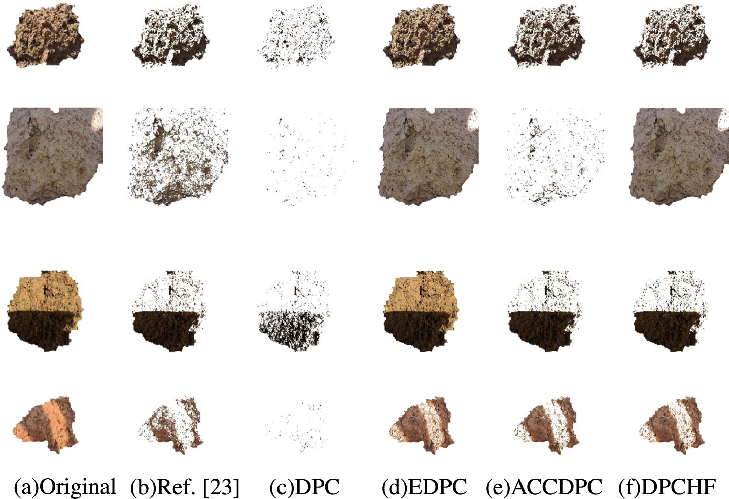
Image results of Experiment 1 with No.4 sample group.

Fig. 6

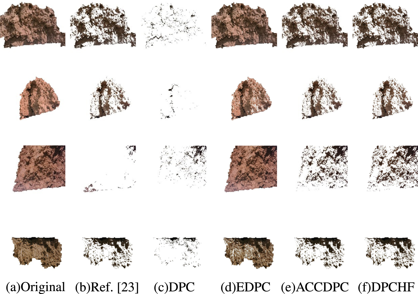
Image results of Experiment 1 with No.13 sample group.

4.4.2 Data results of shadow detection experiment

The accuracy results of shadow detection of Experiment 1, which are described by brightness standard deviation, are written into Table 1.

Table 1
Segmenting accuracy of experiment 1

Sample group Detecting target Ref. [23] DPC EDPC ACCDPC DPCHF

1 shadow 19.7670 7.3320 39.2835 25.2134 17.3651

non-shadow 23.7973 37.0645 12.8311 16.2817 22.6514

2 shadow 20.4383 7.5124 42.3490 24.9416 17.6270

non-shadow 27.9193 40.9858 12.7779 19.8242 25.4602

3 shadow 19.7255 6.1759 48.1615 19.9196 20.1510

non-shadow 32.5296 44.6972 10.5131 22.4307 18.5645

4 shadow 14.9758 6.7777 54.6038 19.7860 19.2684

non-shadow 49.2346 47.9430 11.1330 28.8679 29.2881

5 shadow 19.1365 7.2854 52.1195 20.7878 20.1570

non-shadow 32.4588 48.4304 11.6091 26.2275 26.6957

6 shadow 20.4277 7.4917 42.9366 22.7191 18.9523

non-shadow 29.9495 39.3969 12.2439 22.7790 24.8550

7 shadow 16.8284 7.0073 49.7011 16.9986 15.7356

non-shadow 20.9456 37.8268 16.8904 34.2391 21.4620

8 shadow 19.7538 6.6777 40.7236 22.5447 23.6186

non-shadow 23.6495 39.4011 6.9015 19.9483 18.7728

9 shadow 24.2772 6.4873 35.7311 21.0509 24.6930

non-shadow 26.0649 34.6633 6.9784 19.2186 14.3086

10 shadow 19.9684 6.1347 41.6183 22.1200 22.7985

non-shadow 27.7196 41.2520 10.6964 17.2335 16.3607

11 shadow 24.3484 6.3590 38.5540 22.2750 26.3642

non-shadow 36.1016 38.8839 9.6390 20.6703 15.8876

12 shadow 20.3447 6.6157 40.0290 23.0501 24.0382

non-shadow 24.1755 40.8219 9.5787 18.8676 17.7928

13 shadow 19.0971 5.5470 37.8518 21.1598 21.4568

non-shadow 26.6191 37.1828 8.2332 18.0776 17.4037

14 shadow 18.9068 6.3008 39.0193 20.1011 20.7039

non-shadow 20.5627 38.4048 10.2360 19.2052 18.4632

15 shadow 21.3266 5.1932 40.9771 20.6308 21.0930

non-shadow 32.8910 40.7309 9.4718 17.1656 16.6550

average shadow 19.9548 6.5932 42.9106 21.5532 20.9348

non-shadow 28.9746 40.5124 10.6489 21.4025 20.3081

Sample group	Detecting target	Ref. [23]	DPC	EDPC	ACCDPC	DPCHF
1	shadow	19.7670	7.3320	39.2835	25.2134	17.3651
	non-shadow	23.7973	37.0645	12.8311	16.2817	22.6514
2	shadow	20.4383	7.5124	42.3490	24.9416	17.6270
	non-shadow	27.9193	40.9858	12.7779	19.8242	25.4602
3	shadow	19.7255	6.1759	48.1615	19.9196	20.1510
	non-shadow	32.5296	44.6972	10.5131	22.4307	18.5645
4	shadow	14.9758	6.7777	54.6038	19.7860	19.2684
	non-shadow	49.2346	47.9430	11.1330	28.8679	29.2881
5	shadow	19.1365	7.2854	52.1195	20.7878	20.1570
	non-shadow	32.4588	48.4304	11.6091	26.2275	26.6957
6	shadow	20.4277	7.4917	42.9366	22.7191	18.9523
	non-shadow	29.9495	39.3969	12.2439	22.7790	24.8550
7	shadow	16.8284	7.0073	49.7011	16.9986	15.7356
	non-shadow	20.9456	37.8268	16.8904	34.2391	21.4620
8	shadow	19.7538	6.6777	40.7236	22.5447	23.6186
	non-shadow	23.6495	39.4011	6.9015	19.9483	18.7728
9	shadow	24.2772	6.4873	35.7311	21.0509	24.6930
	non-shadow	26.0649	34.6633	6.9784	19.2186	14.3086
10	shadow	19.9684	6.1347	41.6183	22.1200	22.7985
	non-shadow	27.7196	41.2520	10.6964	17.2335	16.3607
11	shadow	24.3484	6.3590	38.5540	22.2750	26.3642
	non-shadow	36.1016	38.8839	9.6390	20.6703	15.8876
12	shadow	20.3447	6.6157	40.0290	23.0501	24.0382
	non-shadow	24.1755	40.8219	9.5787	18.8676	17.7928
13	shadow	19.0971	5.5470	37.8518	21.1598	21.4568
	non-shadow	26.6191	37.1828	8.2332	18.0776	17.4037
14	shadow	18.9068	6.3008	39.0193	20.1011	20.7039
	non-shadow	20.5627	38.4048	10.2360	19.2052	18.4632
15	shadow	21.3266	5.1932	40.9771	20.6308	21.0930
	non-shadow	32.8910	40.7309	9.4718	17.1656	16.6550
average	shadow	19.9548	6.5932	42.9106	21.5532	20.9348
	non-shadow	28.9746	40.5124	10.6489	21.4025	20.3081

Experiment 2 is that DPCHF executed 10 times. Their average and standard deviation of time cost exhibited in Table 2.

Table 2

Time cost of Experiment 2

Sample group	Ref. [23](s)	DPC(s)	EDPC(s)	ACCDPC(s)	DPCHF(s)
1	0.1533±0.020	0.2690±0.080	0.3183±0.090	0.3785±0.090	0.4898±0.070
2	0.1810±0.040	0.2643±0.030	0.2903±0.060	0.4010±0.080	0.4820±0.070
3	0.1483±0.020	0.2298±0.050	0.2538±0.090	0.3355±0.050	0.4965±0.090
4	0.1325±0.030	0.2490±0.030	0.1993±0.030	0.3545±0.050	0.4718±0.090
5	0.1208±0.010	0.2435±0.050	0.2635±0.060	0.3895±0.060	0.4645±0.080
6	0.1570±0.040	0.2610±0.040	0.2533±0.050	0.3585±0.070	0.4683±0.080
7	0.1130±0.030	0.2130±0.020	0.2100±0.040	0.3130±0.070	0.4880±0.070
8	0.1593±0.010	0.2388±0.020	0.2340±0.050	0.3870±0.060	0.4830±0.080
9	0.1738±0.020	0.2425±0.030	0.2410±0.060	0.3830±0.070	0.4933±0.080
10	0.1445±0.050	0.2238±0.050	0.2818±0.070	0.3393±0.060	0.5335±0.070
11	0.1195±0.030	0.2518±0.030	0.2923±0.080	0.3778±0.070	0.5140±0.090
12	0.1410±0.020	0.2765±0.050	0.2808±0.080	0.3663±0.080	0.5258±0.090
13	0.1360±0.040	0.2543±0.040	0.2880±0.090	0.3040±0.050	0.5228±0.090
14	0.1525±0.040	0.2638±0.040	0.2638±0.070	0.4118±0.090	0.5648±0.090
15	0.1725±0.030	0.2355±0.030	0.2575±0.060	0.3008±0.070	0.4900±0.070
average	0.1470±0.029	0.2478±0.039	0.2619±0.065	0.3600±0.068	0.4992±0.081

4.4.3 Accuracy analysis of shadow detection

Figures 5 and 6 declare that DPCHF algorithm has better segmentation effect than Ref. [23], DPC, EDPC and ACCDPC algorithm.

Table 1 exhibits that the mean of brightness standard deviation of shadow and non-shadow segmented by DPCHF are 20.9348 and 20.3081, and the mean values of brightness standard deviations of shadow and non-shadow segmented by the comparison algorithm (Ref. [23], DPC, EDPC and ACCDPC algorithm) are 19.9548 and 28.9746, 6.5932 and 40.5124, 42.9106 and 10.6489, 21.5532 and 21.4025 respectively. It is seen in Table 1 that the sum of the standard deviation mean of shadow and non-shadow segmented by DPCHF is far less than the result segmented by Ref. [23], DPC, EDPC and DPCHF. It bears out that the accuracy of the DPCHF algorithm is higher.

At the same time, it appears in Table 1 that the standard deviation of shadow cut out by DPC is very small and the standard deviation of non-shadow is very large. It illustrates that partial shadows are carried into non-shadow. Similarly, Ref. [23] is the same as DPC, EDPC is opposite to Ref. [23] and DPC, and partial non-shadows are cut into shadow by it. It has fully emerged in Table 1 that shadows and non-shadow may be misclassified by ACCDPC because the standard deviations of shadow and non-shadow are not nearly equal.

4.4.4 Analysing the time cost and algorithm efficiency

Table 2 appears that the average time cost of 15 groups experimental samples based on DPCHF is 0.4992±0.0806, and the average time cost of 15 groups experimental samples based on comparison algorithm(Ref. [23], DPC, EDPC and ACCDPC algorithm) are 0.1470±0.0287, 0.2478±0.0393, 0.2619±\\ 0.0653, 0.3600±0.068 respectively.

The data of time cost demonstrate that the DPCHF algorithm has the largest average time cost. After research and analysis, it is found that the algorithm in Ref. [23] is a self-defined Otsu algorithm with a single measure, which takes less time. However, this method is mainly effective for regular shadow detection of buildings shadow, and its adaptability of soil shadow detection is very poor, which can not meet the accuracy requirements of soil images shadow detection. DPCHF algorithm in this paper is more time-consuming than DPC, EDPC and ACCDPC, because these three algorithms all use the allocation rule from the original DPC algorithm. DPCHF algorithm uses Fourier series to search for valley points and establish an optimization model to obtain shadow and non-shadow optimal segmenting threshold points. These two steps increase the time cost of the algorithm, but it improves the accuracy of shadow detection in soil image and solves the problem of “domino” error propagation caused by the original DPC algorithm.

The above analyses present that DPCHF algorithm increases the second level time cost solves the “domino” error propagation problem. Hence, it’s worth improving the accuracy of soil image shadow detection.

4.4.5 The detection of full shadow or non-shadow image

The DPCHF algorithm detects full shadow or non-shadow images with the robust samples, and finds the unimodal characteristics of all samples. The unimodal characteristics of the robust sample are Fig. 7.

Fig. 7

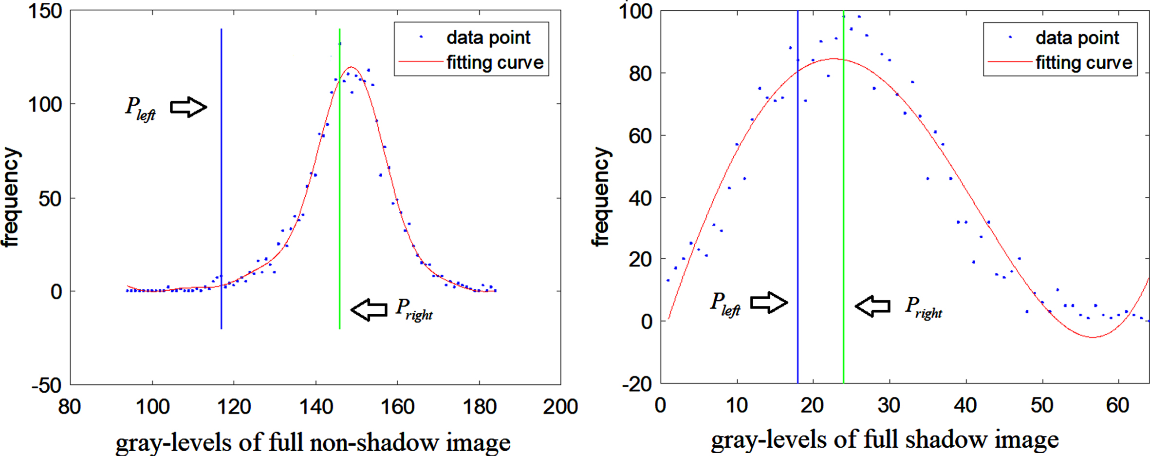
The unimodal characteristics that is detected by DPCHF in Experiment 3.

5 Conclusion

Shadow detection of soil image is a typical binary classifying problem, and its brightness histogram has bimodal characteristics. Thus, a curve of its brightness histogram is fitted, and its two peak points obtain as the clustering centers, and a valley point between its two peak points is optimized as the segmenting threshold for shadow detection. The conclusion of this work is as follows.

(1) Reconstruct the nonparametric density formula and decision value measure for obtaining the clustering center adaptively.

(2) Fourier series are drawn into approximating the brightness histogram, and a part of brightness points are allocated by valley points of the histogram fitting curve.

(3) Establishing an optimizing model to optimize the shadow detection threshold, and the optimized threshold classifies the remaining data. So, the problem of “domino” error propagation caused by the allocating strategy of clustering data based on the original density peak clustering algorithm is effectively solved by the DPCHF algorithm because it is a threshold segmentation.

(4) Simulation results manifest that the DPCHF algorithm has higher detection accuracy for soil image shadow detection than the contrast algorithm and solves the problem of “domino” error propagation. Although it increases the cost of time, this is valuable for the shadow detection of soil images.

Although the effectiveness of the proposed algorithms is promising, some open issues remain to be solved in the future. The time cost of the shadow detection algorithm of soil images can be further improved.

Footnotes

Acknowledgments

This work supported by the Key Science and Technology Research Program (No. KJZD-K201900505) and Chongqing University Innovation Research Group funding (No. CXQT20015) of Chongqing Municipal Education Commission, China.

References

Rodriguez

and Laio

, Clustering by fast search and find of density peaks, Science 6191 (2014), 1492–1496.

Liu

, Wu

, Peng

, et al., Local Peaks-Based Clustering Algorithm in Symmetric Neighborhood Graph, IEEE Access 99 (2019), 1–1.

Zhang

, Lu

Y.H.

and Huang

D.C.

, Weighted hesitant fuzzy clustering based on density peaks, Computer Science 01 (2021), 145–151.

Ding

S.Y.

and Tian

Q.Y.

, Density Peak Clustering Algorithm Based on Ball-Tree, Computer Engineering and Applications 01 (2021), 1–9.

Wang

F.Y.

, Zhang

D.S.

and Zhang

, Adaptive Density Peaks Clustering Algorithm Combining with Whale Optimization Algorithm, Computer Engineering and Applications 03 (2021), 94–102.

Sun

, Tao

, Zheng

, et al., Combining density peaks clustering and gravitational search method to enhance data clustering, Engineering Applications of Artificial Intelligence 85 (2019), 865–873.

, Ding

, Wang

, et al., A fast density peaks clustering algorithm with sparse search, Information Sciences 3 (2020), 554.

Liu

, Huang

, Fei

, et al., Constraint-based clustering by fast search and find of density peaks, Neurocomputing 22 (2019), 223–237.

Zhang

, Dua

, Qu

S.N.

, et al., Adaptive density-based clustering algorithm with shared KNN conflict game, Information Sciences 565 (2021), 344–369.

10.

Wang

Y.Z.

, Wang

, Pang

, et al., A systematic density-based clustering method using anchor points, Neurocomputing 400 (2020), 352–370.

11.

Zhen

, Wang

and Yu

, A Clustering Algorithm with Adaptive Cut-off Distance and Cluster Centers, Data Analysis and Knowledge Discovery 03 (2018), 39–48.

12.

Wang

and Zhang

, Automatically determine density of cluster center of peak algorithm, Computer Engineering and Applications 08 (2018), 137–142.

13.

Hou

and Zhang

, Enhancing Density Peak Clustering via Density Normalization, IEEE Transactions on Industrial Informatics 99 (2019), 1–1.

14.

Jiang

, Zang

, Sun

, et al., Adaptive density peaks clustering based on K-nearest neighbor and Gini coefficient, IEEE Access 99 (2020), 1–1.

15.

Chun

, Li

, Yu

, et al., Effective Density Peaks Clustering Algorithm Based On the Layered K-Nearest Neighbors And Subcluster Merging, IEEE Access 99 (2020), 1–1.

16.

Liang

and Chen

, Delta-density based clustering with a divide-and-conquer strategy: 3DC clustering, Pattern Recognition Letters 1 (2016), 52–59.

17.

Liu

Y.H.

, Ma

Z.M.

and Yu

, Adaptive density peak clustering based on K nearest neighbors with aggregating strategy, Knowledge-Based Systems 1 (2017), 208–220.

18.

Zeng

S.H.

, Tang

W.M.

, Zhan

L.Q.

, et al., Color image segmentation of field purple soil based on adaptive density peaks clustering, Transactions of the Chinese Society of Agricultural Engineering 19 (2019), 200–208.

19.

Flores

K.G.

and Garza

S.E.

, Density peaks clustering with gap-based automatic center detection, Knowledge-Based Systems 206 (2020).

20.

Fang

, Qiu

and Yuan

, Adaptive core fusion-based density peak clustering for complex data with arbitrary shapes and densities, Pattern Recognition 2020(107).

21.

Q.Y.

, Wang

N.C.

and Yi

D.Q.

, Numerical analysis, Issued by Tsinghua University Press, 2008.

22.

Wang

, et al., DB50\/T 796-2017 Classfication and codes for Chongqing soil, Issued by Chongqing Bureau of Technical Supervision, 2017, (in Chinese).

23.

Tsai

V.J.D.

, A comparative study on shadow compensation of color aerial images in invariant color models, IEEE Transactions on Geoscience & Remote Sensing 6 (2006), 1661–1671.