Automatic prediction of coronary artery disease using differential evolution-based support vector machine

Abstract

Coronary artery disease (CAD) is a common heart disease that causes the blockage of coronary arteries. To reduce fatality, an accurate diagnosis of this disease is very important. Angiography is one of the most trustworthy and conventional methods for CAD diagnosis however, it is risky, expensive, and time-consuming. Therefore in this study, we proposed a differential evolution-based support vector machine (SVM) for early and accurate detection of CAD. To improve the accuracy, different data preprocessing techniques such as one-hot encoding and normalization are also used with differential evolution for feature selection before performing classification. The proposed approach is benchmarked with the Z-Alizadeh Sani and Cleveland datasets against four state-of-the-art machine learning algorithms, and a highly cited genetic algorithm-based SVM (N2GC-nuSVM). The experimental results show that our proposed differential evolution-based SVM outperforms all the compared algorithms. The proposed method provides accuracies of 95±1% and 86.22% for predicting CAD on the benchmark datasets.

Keywords

Coronary Artery Disease (CAD)Machine Learning (ML)Differential Evolution (DE)Genetic Algorithm (GA)Support Vector Machine (SVM)Naïve Bayes (NB)Multilayer perceptron (MLP)Classification True positive rate (TRP)False positive rate (FPR)

1 Introduction

Coronary artery disease is the most common fatal heart disease that causes millions of deaths every year. According to the world health organization, 31% of fatality is caused by heart disease [1]. Therefore, a timely and accurate diagnosis of CAD is necessary to reduce this fatality rate. The aim of this research is to combine machine learning and evolutionary computation techniques effectively for diagnosing CAD.

Machine learning is the process that focuses to improve an algorithm’s performance automatically through experience [2]. There is a large variety of machine learning algorithms such as neural networks, support vector machines, logistic regression, decision trees, and many more. The choice of these algorithms depends on the data and research (for which they are going to be used).

The use of machine learning algorithms in healthcare applications is becoming popular day by day. Due to the large amount of data involved in these applications, it is necessary to extract information from them. Recently, Abdar et al. [2] applied 10 traditional machine learning algorithms for CAD diagnosis. In most cases Support Vector Machine (SVM) performed better, and the results of SVM were further improved by using a Genetic Algorithm (GA). The GA with SVM outperformed all other compared methods. Though the results of the GA-based SVM are quite promising; however, there is always room for improvement. Optimal feature selection can help to improve the performance of different classifiers.

To select an optimal set of features, metaheuristics have been widely and successfully used. In order to find the optimal solution, there is a need to have an appropriate balance between exploration and exploitation of the search space.

The main objective of this paper is to build an effective CAD diagnosis system by using machine learning and an effective evolutionary computation-based method. In this study, we proposed a differential evolution-based support vector machine (SVM) for the early and accurate detection of CAD.

Differential evolution (DE) is used to find the optimal set of features by exploring the promising regions of the search space during initial iterations of the algorithm, and then exploiting those regions in the later iterations. Balanced explorative and exploitative capabilities of DE help to escape the local optima and converge to the near-global optimum. Moreover, to improve the accuracy, different data preprocessing techniques such as one-hot encoding and normalization proposed in [2] are also used with differential evolution for feature selection before performing classification.

The proposed method is benchmarked with the Z-Alizadeh Sani and Cleveland datasets against state-of-the-art machine learning methods including multilayer perceptron algorithm, naïve Bayes, random forest, SVM, and a highly-cited genetic algorithm-based SVM (N2GC-nuSVM). The experimental results show that our proposed differential evolution-based SVM classifier outperforms all the compared algorithms for predicting CAD on the benchmark datasets.

The main contributions of this paper are as follows:

In this study, we proposed a differential evolution-based support vector machine (SVM) for the early and accurate diagnosis of coronary artery disease.

The proposed methodology combines effective evolutionary-based and machine learning approaches exploiting the benefits of each method to develop a CAD diagnosis system with improved performance. The differential evolution is used for the optimal selection of features, and SVM classifies those features to detect the CAD effectively.

The proposed differential evolution-based SVM is evaluated on two benchmark datasets against five state-of-the-art classification methods. The experimental results show that the proposed method outperforms all the compared algorithms. The excellent performance against all compared algorithms shows that the proposed differential evolution-based SVM classifier is an effective method for the diagnosis of CAD.

The rest of the paper is organized as follows: literature review and description of the data are presented in section 2. In this section, we reviewed the studies that use machine learning techniques for the detection of heart diseases. In section 3, the proposed methodology is presented. Experimental results obtained from this methodology are presented in section 4. In section 5, conclusions and future work are presented.

2 Literature review

The use of machine learning techniques in the medical field is becoming popular. For the detection of different diseases, machine learning algorithms have been applied to medical datasets. There are some conventional methods available for the detection of heart diseases, i.e., angiography, electrocardiogram, and computerized tomography which are expensive and rely more on medical doctors [3].

Ghandiri et al. [4] proposed a medical expert system that ensembles a particle swarm optimization (PSO) based approach to extract rules for the diagnosis of CAD. They presented boosting mechanism that cooperates between generated fuzzy if-then rules using the PSO metaheuristic. They evaluated their classification technique on the Cleveland data set and obtained 92.5% accuracy [4]. Different data mining and machine learning techniques for CAD detection are presented by Alizadeh Sani et al. in previous years. In all these studies, the best accuracy obtained is 94% by using the sequential minimal optimization (SMO) algorithm [2]. They also achieved competitive accuracy by using different techniques on an extended dataset that contains 500 instances.

Verma et al. presented a hybrid data mining model, where they used PSO with correlation-based feature selection (CFS) on data that is collected from Indira Gandhi medical college, India. They implemented different classification algorithms on selected features. With selected features, multi-layer perceptron (MLP) gives 84.17% accuracy; fuzzy unordered rule induction algorithm (FURIA) gives 80.29% accuracy, and C4.5 gives 77.9% accuracy [5].

Abdar et al. used a genetic algorithm and PSO with 10-fold cross-validation, for two purposes: for classifier’s parameters optimization and for feature selection. They implemented this technique on the Z-Alizadeh Sani dataset and obtained 93.08% accuracy on the training samples by using their proposed method called N2Genetic [2]. Pławiak [6] investigated cardiac disorder by using electrocardiogram (ECG) analysis and an evolutionary neural model. After normalization and feature extraction, he proposed a methodology for a heart disease dataset by using four classifiers: K-nearest neighbor (KNN), SVM, radial basis function neural network (RBFNN), and perturbative neural network (PNN). The evolutionary neural model with SVM gives 90% accuracy for the ECG dataset with 17 classes [6].

A study by Arabasadi et al. presented a hybrid method for accurate detection of cardiovascular disease (CAD). Their methodology increased the performance of the neural network by ten percent. Because they used a genetic algorithm for enhancing the weight, the genetic algorithm suggests better parameters i.e., weights for the neural network. They obtained 93.8% accuracy by using this method [7].

For the prediction of heart disease, Hamdaoui et al. proposed a clinical support system [8]. They applied different machine learning algorithms i.e., K-Nearest Neighbor, Random Forest, Support Vector Machine, Decision Tree, and Naïve Bayes for heart disease prediction, on the data retrieved from medical files. They performed various experiments for prediction on UCI data, and the results show that Naïve Bayes provides the best outcome with both cross-validation and train-test split techniques. It provides an accuracy of 82.17%, and 84.28%, respectively. Rabbi et al. [9] applied different algorithms i.e., K-Nearest Neighbor, SVM, Artificial neural network, and multi-Layer perceptron on Cleveland data, which is split into two equal parts one for training and the second for testing. Compared with other methods, SVM outperformed and obtained results with 85% classification accuracy. Chen and Hengjinda [28] proposed a machine learning technique, which identifies knowledge by constructing pooled area curve for accurate prediction. The experimental results show that the SVM outperforms other methods. Velusamy and Ramasamy [29] developed a novel ensemble approach for the effective diagnosis of CAD. The proposed method combined 3 widely used machine learning classifiers, which are Support Vector Machine, Random Forest, and K-Nearest Neighbor. The performance was benchmarked against state-of-the-art algorithms on the Z-Alizadeh Sani dataset. The suggested ensembled approach outperformed the compared algorithms.

2.1 Dataset description

Dataset used in this study is obtained from Iranian patients. It has 303 records with 54 features and two classes: normal patients and CAD patients [10]. The main features of the dataset are divided into four categories: Demographic, Electrocardiogram, symptom and examination, and laboratory and echo features. The following feature names are shown with their type:

Demographic: Weight, Age, Diabetes Mellitus, EX-Smoker, Current Smoker, Hyper-tension, Family history, Body Mass Index, Dyslipidemia, Airway Disease, Chronic Renal Failure, Cerebrovascular Accident, Congestive Heart Failure, Obesity, Thyroid disease.

Laboratory and Echo: Edema, Systolic Murmur, Typical Chest Pain, Atypical, Weak peripheral Pulse, Exertional Chest pain, Nonagonal CP, Dyspnea, Lung Rales, Diastolic Murmur, Low threshold angina, Blood Pressure, Functional Class, Pulse Rate.

ECG: ST Elevation, Poor R Progression, T Inversion, Q Wave, LVH (Left Ventricular Hypertrophy), ST Depression, Lymph, Rhythm. Symptom and Examination: Lymphocyte, Potassium, Valvular Heart Disease, Blood Urea Nitrogen, Creatine, Low-Density Lipoprotein, Triglyceride, Erythrocyte Sedimentation rate, Neutrophil, High-Density Lipoprotein, Hemoglobin, Platelet, Fasting Blood Sugar, Sodium, Regional Wall Motion Abnormality, Ejection Fraction, Fasting Blood Sugar, White Blood Cell. Twenty-one features are numeric and the rest are binary or categorical; this data is open source and easily available.

3 Methodology

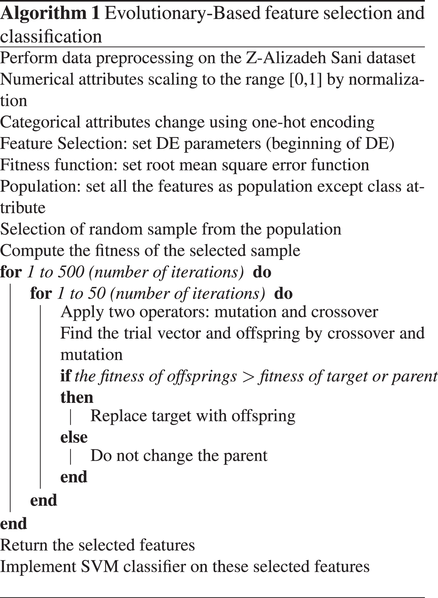
In the present communication, an innovative approach to detect CAD is presented. The overall algorithmic steps are given in Algorithm 1. In this section, the following proposed methodology is described in detail.

3.1 Preprocessing

Missing values: no missing values are found in the data.

One hot encoding: is performed on categorical features to convert them into binary vectors. For each category, there is a column that is filled with binary values. For example, if a categorical feature has four categories: normal, mild, severe, and moderate, there are four columns with each category having binary values.

Normalization: is performed on numerical features to standardize them from 0 to 1.

Feature selection: 22 out of 54 features are selected from data by using differential evolution.

3.2 Different machine learning techniques on dataset:

We have implemented different machine learning algorithms on data after preprocessing, i.e., genetic algorithm SVM, Naïve Bayes, random forest, linear regression, logistic regression, and multilayer perceptron. From all implemented algorithms, the genetic algorithm with SVM provides good results with 93% accuracy. An explanation of all tested algorithms is given below.

3.2.1 Genetic algorithm

It is the search algorithm, inspired by ‘Darwin’s theory [11]. This algorithm selects the fittest individuals for producing offspring in the new generation. The steps of the genetic algorithm are as follows:

Initialization of population.

Calculate the fitness of individuals.

Selection of individuals.

Crossover: select two individuals and perform a swap gene between them.

Mutation: select one individual and mutate a gene in it.

The parameters used for differential evolution are as follows:

Population size: 300 individuals;

Number of generations: 100;

Crossover probability: 0.8;

Mutation probability: 0.2;

Fitness function: accuracy and F-score.

3.2.2 SVM

SVM is the supervised machine learning classification model; use to classify two-class problems [12]. It takes the data points and finds a hyperplane that best separates these data points. This hyperplane is called a decision boundary. Everything on one side of this decision boundary represents one class and the other side of the boundary represents the other class.

Support vectors are the data points that affect the location and orientation of the hyperplane. These points are closest to the hyperplane; where the margin shows that there should be a maximum distance of the hyperplane from the support vectors of both classes.

3.2.3 Naïve bayes

Naïve Bayes is not a single algorithm; it is the combination of algorithms that depends on Bayes theorem. Bayes theorem finds the probability of an event by using the probability of the previous event that has occurred. Its principle is that all the features are independent of each other, and all the features contain the same weight.

3.2.4 Random forest

Random forest is the most flexible supervised learning algorithm [13], which consists of a forest of randomly comprised trees. It can be used for both the classification as well as regression problems. A greater number of trees can cause overfitting. We have used fifty estimators for CAD prediction. The working of random forest is described below:

First of all, select the random samples.

Create a decision tree corresponding to each random sample.

Get prediction accuracy from each decision tree.

Perform voting for each result.

Select the result with more votes.

3.2.5 Multi-layer perceptron

Multi-layer perceptron is an artificial neural network that contains three types of layers: input layer, hidden layers, and output layer. There is only one input and an output layer but hidden layers can be more than one. The input layer has neurons that feed input to the model. Hidden layers may have more than one neuron that most of the time uses a non-linear function called ‘activation function’. Multi-layer perceptron is a supervised learning algorithm and for training it uses backpropagation. For the prediction of CAD, we used a multi-layer perceptron with three hidden layers. Each of these hidden layers has thirteen neurons with ReLU (rectified linear unit) as activation function and calculates RMSE in the output layer. The above Figure 1, shows the process of multi-layer perceptron:

Fig. 1

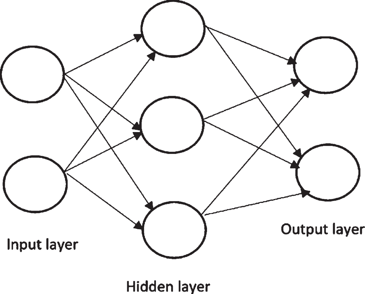
Graphical representation of Multi-layer perceptron.

3.3 Differential evolution for feature selection

There can be redundant and dependent features in large datasets that can affect the performance of machine learning algorithms [16]. A lot of algorithms are available for feature selection such as the wrapper method, genetic algorithm, and particle swarm optimization. Here we are using a low-cost and efficient evolutionary computation algorithm, differential evolution for feature selection.

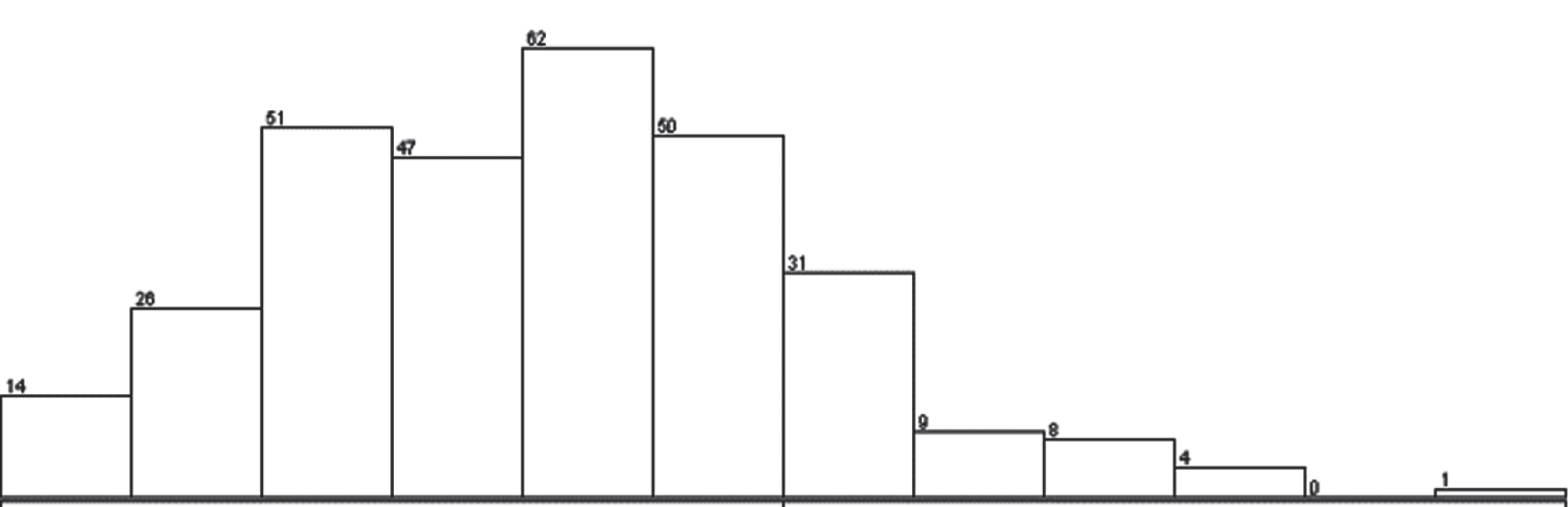
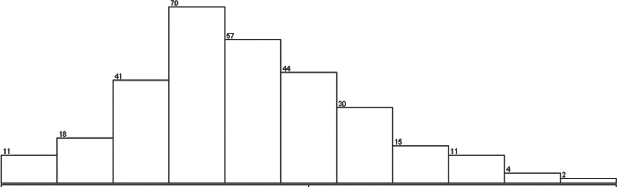
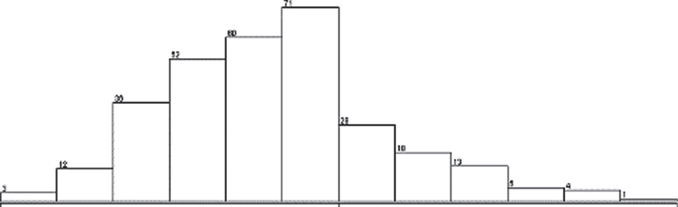
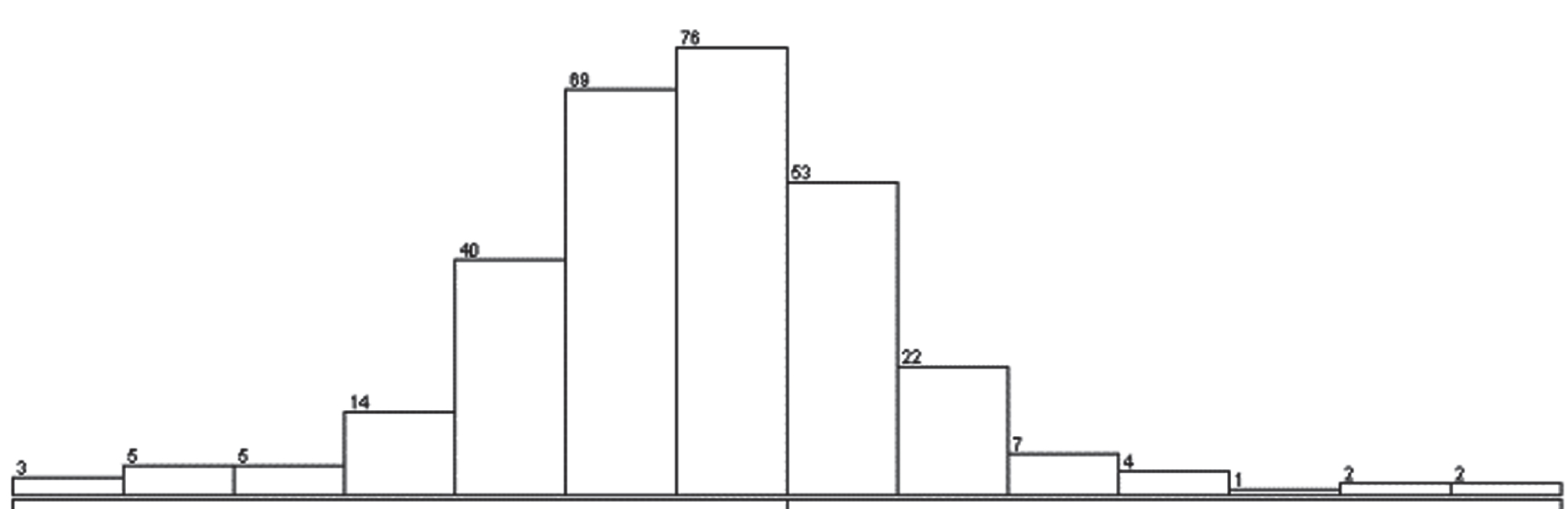
Differential evolution is a population-based search strategy developed by Storn and Price in 1995. It is a novel approach to get a multitude of advantages when applied to a dataset. It optimizes the objective function and provides the array global optima. The distribution of selected attributes is shown from Figs. 10–19.

The differential evolution algorithm framework consists of four steps:

Initialization: The first step of DE is to find the global optimum solution in D-dimensional space. The initial solutions for the problem consist of real-valued parameter vectors of population size. In the d-th iteration, every i-th individual solution of differential evolution can be represented as D-dimensional vector as: $X_{i}^{d} = X_{i, 1}, X_{i, 2}, . . . ., X_{i, D} .$ The initial population condition starts at d = 0. The initial candidate solutions generated on the basis of the lower and upper limit boundaries of the solution search space as follows: $X_{\min} = X_{\min, 1}, X_{\min, 2}, \dots, X_{\min, D};$ $X_{\max} = X_{\max, 1}, X_{\max, 2}, \dots, X_{\max, D};$ For d-th solution, the e-th dimensional component can be initialized by randomly generating a value in between the Xmax,e and Xmin,e as: $X_{d, e}^{(0)} = X_{\min, e} + {rand}_{d, e} [0, 1] (X_{\max, e -} X_{\min, e});$ where rand [0, 1] generate any real value between 0 and 1.

Mutation: It is the perturbation process that is performed on selected variables. From different mutation strategies, we used DE/best/1: $Y_{i}^{t} = X_{best}^{t} + F (X_{r 1}^{t} - X_{r 2}^{t});$ where X_r1 is the base vector and X_r2 is is the randomly selected vector to construct the mutant vector. F is the probability of mutation.

Crossover: In this step the target and the mutant vector cross their components to construct the trial vector. In this work we are using uniform crossover scheme to find trial vector as: $T_{i}^{t} = {\begin{matrix} Y_{i}^{t}, if r {and}_{i, j} [0, 1] \leq cr or j = k \\ X_{i}^{t}, otherwise \end{matrix}$ where cr is the cross rate that have value in [0, 1].

Selection:

This process determine which solution will survive in the next iteration, either trial solution or target solution. The selection process of differential evolution is described as: $X_{i}^{t + 1} = {\begin{matrix} T_{i}^{t}, if f (T_{i}^{T}) \leq f (X_{i}^{t}) \\ X_{i}^{t}, otherwise \end{matrix}$

The parameters used for differential evolution are as follows:

Bounds: Bounds are the coordinate values for an achievable solution. They have an upper limit and a lower limit; the selected bound limit is (-5, 5) for all features.

Population size: population size is 50.

Iterations: 500 iterations.

Fitness function: root mean square error (RMSE) is optimized for feature selection: $RMSE = \sqrt{\frac{1}{N} \sum_{i = 1}^{N} (\hat{x_{i}} - x^{s} {quo}_{i})^{2}}$ where x_i is the actual value, x^squo_i is the predicted value, and N is total number of instances.

Weight vector: used to calculate predicted values and it contains a 0.01 weight value for every feature.

Mutation: 0.2 probability of mutation.

Crossover probability: 0.8.

The complexity of differential evolution in terms of notation is:

The complexity of DE = O (G_max * D * NP).

Here G _max is the maximum number of generations, D is the dimension of the decision variable and NP is the population size. In our case, the complexity of DE would be O(500*57*50). Figure 2 presents all the steps performed in this technique to achieve better results.

Fig. 2

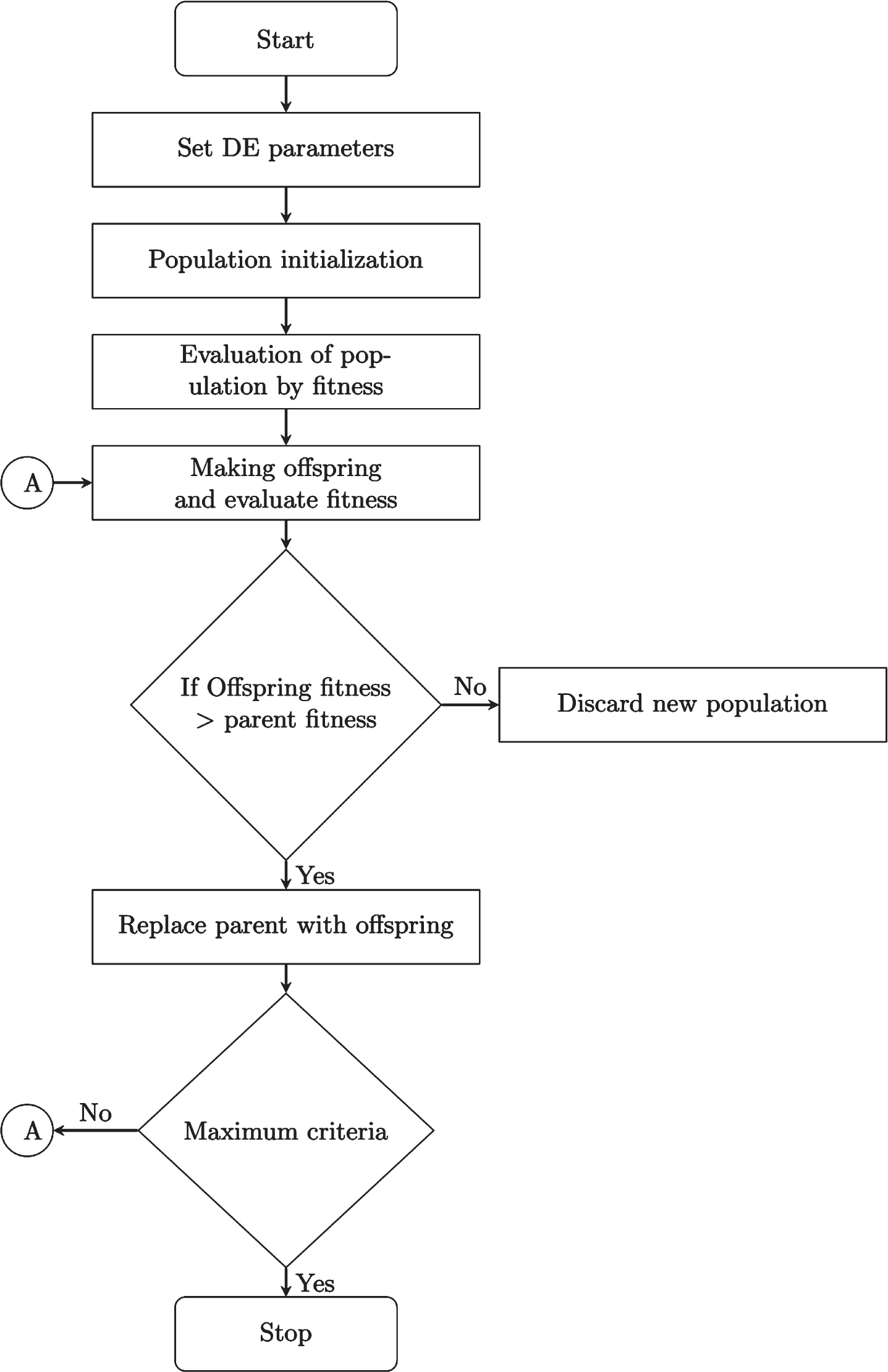
Workflow of differential evolution.

3.4 Splitting of data

We split data into two parts: training, and testing. The training data is used to train the classifier while testing data is used to analyze the performance of the classifier on unseen data.

Training data: 80% randomly selected instances from the data.

Test data: 20% randomly selected instances from the whole dataset.

3.5 Classification

SVM classifier is trained on the training dataset for the classification of CAD and normal patients.

The trained SVM classifier is evaluated on the test data.

The parameters used for SVM are as follows:

Kernel: linear;

Probability: True;

Degree: 4;

Penalty parameter: 0.3.

3.6 Evaluation

The evaluation results are based on the accuracy calculated as follows:

Accuracy= (TP+TN)/(TP+FP+TN+FN);

where TP stands for true positive, CAD patients that are predicted to have CAD disease. TN stands for true negative, normal people that are predicted as normal. FP is for false positive, CAD patients that are predicted normal. FN stands for false negative, normal people that are predicted as CAD patients.

4 Results and discussion

In this section, an experimental evaluation of the results is presented. The Proposed algorithm is coded in Anaconda with python (language) and is run on a Core i5-4300U with 8 GB RAM. As described earlier, from all the tested algorithms, the genetic algorithm provides the best results with SVM; as shown in Table 1, where the fitness function is the accuracy. Moreover, we have compared the proposed method with other machine learning algorithms using Accuracy, F-score, and Area Under Curve (AUC) in Table 3.

Table 1
The accuracy obtained by using a genetic algorithm with SVM on training and testing data

Accuracy for training data Accuracy for testing data

93% 90%

Accuracy for training data	Accuracy for testing data
93%	90%

Differential evolution is an excellent evolutionary algorithm that is mostly used for optimization. In this work, differential evolution is used to select the features by optimizing an error function, i.e. Root Mean Square error, where twenty-two (22) features are selected by using this technique.

In DE, each of the individuals is coded with a vector of n binary numbers, where n is the total number of features of the problem to be solved. If the value of a particular feature is 1, it means that feature is selected and 0 otherwise. The objective of each algorithm is to select the optimal subset of features in such a way that the cost function of the classifier (RMSE) should be minimized. The optimal subset of features will give the minimum RMSE, which is the average of the squared deviation of the predicted values from the actual values of the given dataset. If we compare the feature selection process in DE and GA, the operators in DE help to maintain an appropriate balance between exploration and exploitation to solve the problem effectively. DE used the concept of differential vectors, and in each iteration, the solutions are updated using the difference of vectors (solutions). During the early stages of the evolution, the difference between two vectors (solution) is large, which aids in exploring a range of distant areas of the solution space. However, with the passing iterations, the difference between the two solutions keeps on decreasing, and this assists in exploiting the already discovered potential areas of the solution space. This suitable balance between exploitation and exploration helps DE to find the optimal subset of features in a reasonable time.

DE output for features:. SVM classifier provides the best accuracy results when implemented on these selected features. Table 2 shows the results obtained by SVM.

Table 2

The accuracy obtained by using DE algorithm with SVM on training and testing data

Accuracy for training data	Accuracy for testing data
93±1%	90±1%

One of the Z-Alizadeh Sani research reported 96.40% accuracy but this is for an extended dataset [17]. In this paper, we are using a normal dataset, which has 303 instances while the extended dataset has 500 instances.

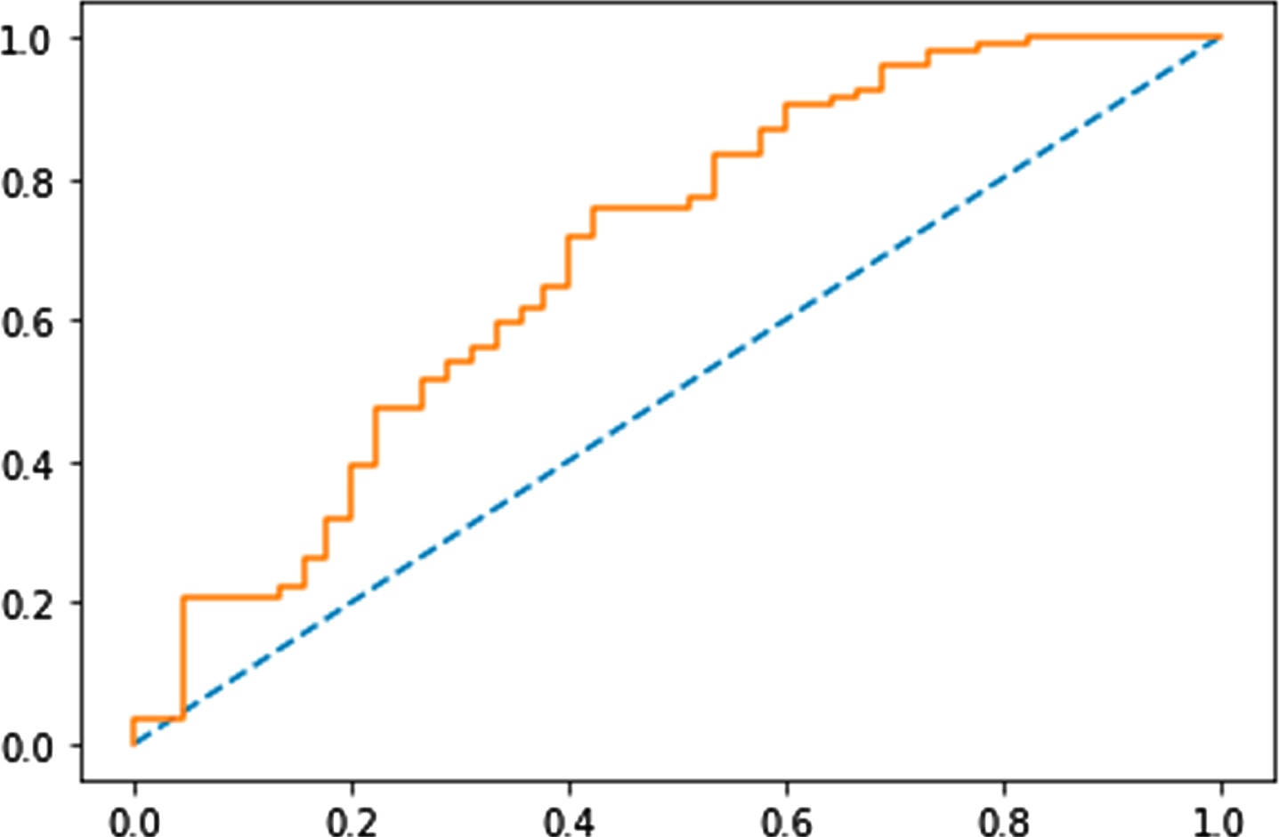
Figures 3–6 show the Receiver Operating Characteristics (ROC) curves of multi-layer perceptron, random forest, Naïve Bayes, and SVM classifiers, respectively. Figures 7 and 8 show the graphical representation of two models: using GA with SVM, and DE-based SVM through the ROC curves, respectively. ROC curve uses to show the trade-off of usefulness between true-positive rate (TPR) and false-positive rate (FPR). The area under the curve represents the correctness of the model on the dataset. Figure 4 shows the ROC curve for the multi-layer perceptron which has 0.701 Area Under Curve (AUC) for the Sani Dataset. In Fig. 4, with n-estimators=25, the AUC for the random forest is 0.851. Similarly, in Figs. 5, 6, we can see AUC scores of 0.873, and 0.894 for Naïve Bayes, and SVM classifiers, respectively. The ROC curve for GA with SVM is presented in Fig. 9 with an AUC score of 0.931. Moreover, we can see that the proposed method (DE with SVM) outperforms all other compared algorithms with an AUC score of 0.950 (almost 2.2% improvement over the existing GA with SVM method). Furthermore, Table 3 represents the accuracy and F-score comparison of all the compared algorithms on two datasets. We can see that the proposed method outperforms all the compared algorithms with accuracy and F-score of 95±1 %, and 92.13 % for the Sani dataset, whereas 86.22 %, and 82.53 % for the Cleveland dataset. The proposed differential evolution based SVM classifier is robust, it can handle a large number of features and training instances. The differential evolution (DE) is used to select the optimal subset of features from a pool of features, and the SVM classifier provides accurate detection of CAD. The suggested DE maintains an appropriate balance between exploration and exploitation effectively

Fig. 3

ROC curve for multi-layer perceptron.

Fig. 4

ROC curve for random forest.

Fig. 5

ROC curve for Naïve Bayes.ROC curve for SVM.

Fig. 6

ROC curve for SVM.

Fig. 7

ROC curve of GA with SVM.

Fig. 8

ROC curve for DE with SVM.

Fig. 9

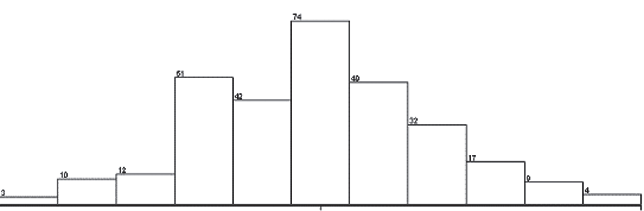
Variation WEIGHT attribute.

Table 3

The performance of the algorithms is evaluated using accuracy, F-score, and AUC. The -, ≈ and + signs depict that the results of DE with SVM are significantly worse, similar, or better than the current results, respectively (using a 95% confidence level in the T-test)

Algorithms	Models	MLP	Random Forest	NB	SVM	GA with SVM	DE with SVM
Sani Dataset	Accuracy%	70+	85+	87+	89.4+	93+	95±1
	F-Score%	63.1+	79.23+	84.5+	85.03+	90.61+	92.134
	AUC	0.701+	0.851+	0.873+	0.894+	0.931+	0.950
Execution time	Training	5.326510	4.835292	6.67783	3.895739	9.631887	9.052478
Cleveland Dataset	Accuracy%	65.23+	84.12+	83.60+	85.72+	85.72+	86.22
	F-Score%	62.01+	80.94+	79.34+	81.20+	81.20+	82.53
Execution time	Training	3.175293	2.627187	3.445025	3.335700	7.684005	7.57373
+: DE with SVM performs better than the compared algorithm (with 95% confidence level)
-: DE with SVM performs worse than the compared algorithm (with 95% confidence level).
≈: DE with SVM performs equally in the comparison.

In order to see the statistical significance of the results, a statistical comparison of the compared algorithms with the proposed technique (DE with SVM) at the confidence level of 95% has been shown in Table 3. The performance of the algorithms is compared using the one-tail t-test. We find the p-values corresponding to each algorithm. All the p-values in Table 4 are less than 0.05 (significant level). The t-test results show that the proposed algorithm performs significantly better than all the compared algorithms on all problem instances. The statistical significance test shows that the proposed technique, which is a hybrid of DE and SVM, has a significant impact on improving the quality of the solutions obtained.

Table 4

P-values corresponding to each algorithm (one tail t-test)

Algorithm	p-value
Proposed algorithm with MLP	0.00001
Proposed algorithm with random forest	0.0001
Proposed algorithm with NB	0.0001
Proposed algorithm with SVM	0.0002
Proposed algorithm with GA	0.0004

4.1 Advantage of the proposed model:

The model presented in this paper provides us with greater accuracy as well as a low cost of time. Other methods are more time-consuming for example GA for the feature selection and classifier’s parameter optimization [2].

4.2 Limitations:

The proposed model should be tested on a large dataset. As our data have 303 instances so there can be a chance of overfitting when trying to train it on more complex deep and machine learning (algorithms).

4.3 Distribution of all variables selected by de:

The distribution of a feature shows the possible values of that feature and how often those values occur. Most of the features that are selected through differential evolution look like bell-shaped as shown in Figs. 9–11, 13–17. Several models and statistical methods assume that the underlying data should be normally distributed.

Fig. 10

Variation of BMI attribute.

Fig. 11

Variation OBESITY attribute.

Fig. 12

Variation of BP.

Fig. 13

Variation of LDL attributVariation of K attribute.

Fig. 14

Variation of K attribute.

Fig. 15

Variation of NA attribute.

Fig. 16

Variation of LYMPHVariation of NEUT attribute attribute.

Fig. 17

Variation of NEUT attribute.

Fig. 18

Variation of VHD-N attribute.

5 Conclusion and Future Work

Coronary artery disease (CAD) is the most common heart disease. In this work, we presented a methodology for the earlier detection of CAD by using a combination of evolutionary and machine learning algorithms. Firstly, we preprocessed our data with one hot encoding (for categorical features) and normalization (for numerical features). On preprocessed data, we implemented different classification techniques to compare their results and obtained 93% maximum test accuracy for the Z-Alizadeh Sani dataset and 85.72% for the Cleveland dataset. In this work, we also presented a new approach that uses differential evolution for feature selection and SVM for classification. We performed all the work on the Z-Alizadeh Sani and Cleveland heart disease datasets. After feature selection, we split data into two parts: one for training and the other for testing. We found that our methodology provides 93±1%, and 86% accuracy on the test data samples of Z-Alizadeh Sani and Cleveland respectively. Our results show that the proposed methodology can be successfully applied to the healthcare datasets for the accurate detection of coronary artery disease. In the future, we plan to test the proposed method with a large dataset to overcome the chances of overfitting. To make data more suitable for classification algorithms, other preprocessing techniques can be applied. We plan to use the presented method with other machine learning and deep learning algorithms to improve the accuracy of CAD prediction.

Footnotes

Acknowledgment

We would like to thank Ms. Rida Mahmood for her help in paper formatting.

References

“WHO,” WHO.int, [Online]. Available: https://www.who.int/healthtopics/cardiovascular-diseases#tab=tab-1 [Accessed 10 1 2021].

Abdar

, ksiazek

, Acharya

U.R.

, Tan

, Makerenkov

and Plawiak

, A new machine learning technique for an accurate diagnosis of coronary artery disease, Computer Methods and Programs in Biomedicine 162 (2019), 104992.

Qin

, Guan

and Wang

, Application of ensemble algorithm integrating multiple criteria feature selection in coronary heart disease detection, Biomedical Engineerin: Applications, Basis and Communications 29(6) (2017), 11.

Hedeshi

N.G.

and Abadeh

M.S.

, An expert system working upon an ensemble pso-based approach for diagnosis of coronary artery disease, 18th Iranian Conference Biomedical Engineering (2011), 14–16.

Verma

, Srivastava

and Negi

P.C.

, A hybrid data mining model to predict coronary artery disease cases using non-invasive clinical data, Journal of Medical System 40(7) (2016).

Pławiak

, Novel methodology of cardiac health recognition based on ecg signals and evolutionary-neural system, Expert Systems with Applications 99 (2018), 334–349.

Arabasadi

, Alizadehsani

, Roshanzamir

, Moosaei

and Yarifard

A.A.

, Computer aided decision making for heart disease detection using hybrid neural network-genetic algorithm, Computer Methods and Programs in Biomedicine 141 (2017), 19–26.

Hamdaoui

H.E.

, Boujraf

, Chaoui

N.E.H.

, Maaroufi

, A clinical support system for prediction of heart disease using machine learning techniques, 5th International Conference on Advanced Technologies, 2020.

Rabbi

M.F.

, Uddin

M.P.

, Ali

, Kibria

, Afjal

M.I.

, Islam

M.S.

and Nitu

A.M.

, Performance evaluation of data mining classification techniques for heart disease prediction, American Journal of Engineering Research 7(2) (2018), 278–283.

10.

Alizadehsani, UCI machine learning repository,Center for machine Learning and Intelligent systems, Archive.ics.uci.edu, [Online]. Available: https://archive.ics.uci.edu/ml/datasets/Z-Alizadeh+Sani. [Accessed 5 2 2020].

11.

“Introduction to Genetic Algorithm”; Towards Data Science, [Online]. Available: https://towardsdatascience.com/introduction-to-genetic-algorithmsincluding-example-code-e396e98d8bf3. [Accessed 15 5 2020].

12.

“Support Vector Machin”; Analytics Vidhya, 9,[Online]. Available: https://www.analyticsvi-dhya.com/blog/2017/09/understaing-support-vector-machine-example-code/. [Accessed 10 5 2020].

13.

Understanding of Random Forest, Towards Data Science, [Online]. Available: https://towardsdatascience.c-om/understanding-random-forest-58381e0602d2. [Accessed 10 5 2020].

14.

“Linear Regression,” Stat Yale Education, [Online]. Available: www.stat.yale.edu/Courses/199798/101/linreg.htm. [Accessed 23 10 2020].

15.

Logistic regression for machine learning, Machine Learning Mastery, [Online]. Available: https://machinelearningmastery.com/logistic-regression-for-machine-learning/. [Accessed 25 9 2020].

16.

Palmer, Wang, Backman, Winblad, Fratiglioni, Differential evolution of cognitive impairment in nondemented older persons: results from the kungsholmen project, Experts Systems with Applications 99 (2018), 334–349.

17.

Alizadehsani

, Hosseini, Khosravi, Khozeimeh, Roshanzamir and Sarrafzadegan, Nahavandi, Non-invasive detection of coronary artery disease in high-risk patients based on the stenosis prediction of separate coronary arteries, Journal of Biomedicine 162 (2018), 119–127.

18.

Alizadehsani

, Habibi, Sani, Mashayekhi, Boghrati and Ghandeharioum, Bahadorian, Diagnosis of coronary artery disease using data mining based on lab data and echo features, Journal of Medical and Bioengineering 2(3) (2012), 133.

19.

Alizadehsani

, Habibi, Zahar, Mashayekhi, Boghrati and Ghandeharioum, Khozeimeh, Fariba, Diagnosis of coronary artery disease via data mining algorithms by considering laboratory and echocardiography features, Official Journal of Rajaie Cardiovascular Medical and Research Center 2(3) (2013), 133–139.

20.

Mastoi, Wah, Raj, Iqbal, Automated diagnosis of coronary artery disease: a review and workflow, Hindawi Cardiology Research and Practice (2018), 9.

21.

As, A comparison of multiple classification methods for the diagnosis of parkinson disease, Expert Systems with Applications 37(2) (2009), 1568–1572.

22.

Alizadehsani

, Hosseini, Boghrati, Ghandeharioum and Khozeimeh, Z. Sani, Exerting cost-sensitive and feature creation algorithms for coronary artery disease diagnosis, International Journal of Knowledge Discovery in Bioinformatics 3(1) (2012), 59–79.

23.

Alizadehsani

, Zangooei, Hosseini, Habibi, Khosravi and Roshanzamir, Khozeimeh, Sarrafzadegan, Nahavandi, Coronary artery disease detection using computational intelligence methods, Journal of Biomedicine 109 (2016), 187–197.

24.

Chattopadhyay, Mishra, Goswami, Feature selection using differential evolution with binary mutation scheme, International Conference of Microelectronics; Computing and Communicatio (2016), 6.

25.

Detrano, Steinbrunn, Pfisetrer, Scmid, Sandhu, Guppy and Lee, Froelicher, International application of a new probability algorithm for the diagnosis of coronary artery disease, The American Journal of Cardiology 64(5) (1989), 304–310.

26.

Luukka, Lampinen, A classification method based on principal component analysis and differential evolution algorithm applied for prediction diagnosis from clinical EMR heart data sets, Computaional Intelligce in Optimization (2010), 21.

27.

Nandalur

, Dwamena, Choudhri and M. Nandalur, Carlos, Diagnostic performance of stress cardiac magnetic resonance imaging in the detection of coronary artery disease: A meta-analysis, Journal of American College of Cardiology 50(14) (2007), 1343–1353.

28.

Chen

J.I.Z.

and Hengjinda

, Early prediction of coronary artery disease (cad) by machine learning method-a comparative study, Journal of Artificial Intelligence 3(01) (2021), 17–33.

29.

Velusamy

and Ramasamy

, Ensemble of heterogeneous classifiers for diagnosis and prediction of coronary artery disease with reduced feature subset, Computer Methods and Programs in Biomedicine 198 (2021), 105770.

Automatic prediction of coronary artery disease using differential evolution-based support vector machine

Abstract

Keywords

1 Introduction

2 Literature review

2.1 Dataset description

3 Methodology

3.1 Preprocessing

3.2 Different machine learning techniques on dataset:

3.2.1 Genetic algorithm

3.2.2 SVM

3.2.3 Naïve bayes

3.2.4 Random forest

3.2.5 Multi-layer perceptron

3.5 Classification

3.6 Evaluation

4 Results and discussion

Table 1 The accuracy obtained by using a genetic algorithm with SVM on training and testing data Accuracy for training data Accuracy for testing data 93% 90%

4.2 Limitations:

4.3 Distribution of all variables selected by de:

Footnotes

Acknowledgment

References

Table 1
The accuracy obtained by using a genetic algorithm with SVM on training and testing data

Accuracy for training data Accuracy for testing data

93% 90%