A fault diagnosis method of rolling element bearing based on improved PSO and BP neural network

Abstract

Aiming at the inherent defects of BP neural network in the field of rolling bearing fault diagnosis, based on the optimization of particle swarm optimization algorithm, this paper uses a variety of optimization strategies to optimize the particle swarm optimization algorithm, and then uses the optimized particle swarm optimization algorithm to optimize the BP neural network. Therefore, a new fault diagnosis method (Dual Strategy Particle Swarm Optimization BP neural network, DSPSOBP) is proposed. DSPSOBP fault diagnosis method is mainly divided into two steps. The first step is EMD decomposition of vibration signal, and the second step is to classify rolling bearing faults by using BP neural network optimized by Double Strategy Particle Swarm Optimization algorithm. Experiments show that DSPSOBP has stronger advantages than BP neural network basic fault diagnosis model.

Keywords

Bearing fault diagnosis BP neural network optimization algorithm particle swarm optimization

1 Introduction

The intelligent diagnosis method based on neural network refers to the use of neural network as the fault diagnosis method of equipment, using the fault tolerance and nonlinear mapping of neural network to learn the nonlinear relationship of equipment faults, establish a diagnosis model for equipment failure, and realize accurate diagnosis of equipment failure. Most of its research results are about pattern recognition, but a small number of them are biased towards failure prediction. The more basic neural networks mainly include BP (Back Propagation) neural network, RBF (Radical Basis Function) network, etc. Among them, BP neural network is a network that can perform “feedforward”. In addition to using the basic network structure for forward propagation, the most The outstanding feature is the ability to propagate errors backwards. Because of this feature, the BP neural network can be unique in the neural network family. The BP neural network has a strong ability to learn simple patterns and has a low storage cost. Due to the existence of these two characteristics, BP neural network can have a place in the field of fault diagnosis.It is proposed to use BP neural network for fault diagnosis of crusher. Lian Cheng et al. proposed to use BP neural network for fault diagnosis of crusher [1]. But in the field of fault diagnosis, it is more applied in the field of bearing fault diagnosis. Li Jet al. proposed a BP neural network method when solving the problem of rolling bearing fault diagnosis [2]. Y Sun et al. proposed a method of combining principal component analysis with BP neural network for bearing fault diagnosis [3]. Lin Shuiquan et al. proposed a time-domain fault diagnosis method. And then the result of rolling bearing fault classification is obtained through BP neural network [4]. N Zhang et al. proposed using BP neural network as fault classifier [5].

With the improvement of accuracy requirements for fault diagnosis, the basic BP neural network fault diagnosis model can no longer fully meet the requirements of equipment fault diagnosis due to the shortcomings of BP neural network such as being easily trapped in local minimums and relatively slow convergence speed. In order to solve the problems existing in the BP neural network and improve the accuracy of the algorithm to solve the fault diagnosis problem, the research direction has begun to change, and it is developing in the direction of seeking to integrate with other algorithms. Qian Zhiyuan proposed to optimize the fault diagnosis method based on BP neural network through genetic algorithm, which provides a new method and idea for solving the problem of fault diagnosis [6]. Wen Zhou et al. proposed a sliding bearing fault diagnosis method using the Mind Evolutionary Algorithm (MEA) to optimize the BP neural network [9]. M Xiao et al. Proposed to optimize BP neural network with beetle algorithm [10].

When the combination of a single algorithm can not produce good results, someone proposed to further improve the optimization algorithm and apply it to the field of bearing fault diagnosis, so as to further improve the performance of BP neural network in the field of bearing fault diagnosis. Guo Wenqiang et al. proposed a neural network diagnosis method combining PSO and GSA [10]. Feng Yufang et al. constructed a rolling bearing fault diagnosis model (IQABC-BP) that combines improved quantum bee colony algorithm and BP neural network [11]. Wang Yuwei et al. proposed a fault identification method using wavelet packet and improved genetic algorithm to jointly optimize neural network [12]. Ma Chao et al. proposed a combination of resampling method and CSBP neural network method to diagnose faults in rolling bearings [13]. Cui Pengyu et al. proposed a method to improve parameters using an improved bat algorithm, and constructed a new fault diagnosis system [14]. Zhang Ning et al. proposed a fault diagnosis method (ADAFSA-BP) using an improved fish school algorithm to optimize neural networks [15]. Y Zhang et al. Proposed a bearing fault diagnosis method based on BP-MLL [17]. Liu Junfeng et al. Proposed the method of combining FSC-MPE with BP neural network [18]. Xu Zifei et al. Proposed the diagnosis method of WOA-IVMD combined with neural network [19].

However, the above research lacks the combination of bearing fault feature extraction and optimized algorithm. Therefore, this paper proposes a new bearing fault diagnosis method (Dual Strategy Particle Swarm Optimization BP neural network, DSPSOBP).

2 The basic principles of BP neural network and PSO algorithm

2.1 EMD

In the late 1990s, Huang proposed empirical mode decomposition (EMD). This algorithm can decompose the characteristics of the signal itself, adaptively decompose the frequency components of different scales in the non-stationary signal in turn, and decompose them into several intrinsic mode functions (IMF), The decomposition order of these IMF functions is from high frequency to low frequency. These IMF components can reflect the inherent properties of the original signal.

The decomposition formula of EMD algorithm is as follows: $x (t) = \sum_{i = 1}^{n} c_{i} + r_{n}$ (1)

Where x (t) is the signal, c_i is the IMF component and r_n is the residual component.

This paper also uses the correlation principle to screen the IMF components. The calculation formula of the correlation coefficient is as follows: $ρ (x, y) = \sum_{i = 0}^{n} x (i) y (i) / \sum_{i = 0}^{n} x (i) \sum_{i = 0}^{n} y (i)$ (2)

Where x (i) and y (i) are two time series, i is the sequence length, and the value range is (0, n).

2.2 BP neural network

BP neural network is the most basic neural network, usually three-layer structure, namely input layer, hidden layer, output layer. The basic network structure is shown in Fig. 1. In the forward training application, the samples will be conducted layer by layer in order, the order is: input layer ->hidden layer ->output layer. If there is a big gap between the output result and the expected value, the second learning process-error back propagation will begin. That is, the weight and threshold of the neural network are adjusted repeatedly through the error function until a satisfactory result is obtained.

The main idea of the BP algorithm is to divide learning into four processes: the mode propagation process, the input mode propagating from the input layer through the hidden layer to the output layer; the process of error back propagation, the expected output of the network and the network reality The error signal of the output difference, if the error signal is relatively large, the back propagation process of the connection weight error will be corrected layer by layer from the output layer through the hidden layer to the input layer; the memory training process, from the mode forward propagation and the error backward propagation The memory training process is repeated alternately and the weights are continuously adjusted; in the state of learning convergence, the network will tend to converge, that is, the global error of the network tends to the minimum value, or the process of ending at the preset learning times.

Due to space reasons, only two important formulas are listed. The first formula belongs to the forward propagation process, and the second formula belongs to the back propagation process.

Fig. 1

BP neural network structure diagram.

The forward transmission output layer formula of BP neural network is as follows: $I_{j} = \sum_{i = 1} w_{ij} O_{j} {+ θ}_{j}$ (3) $O_{j} = f (I_{j}) = \frac{1}{{1 + e}^{I_{j}}}$ (4) where I_j is input, O_j is output, w_ij is weight, θ_j is offset.

The reverse transmission output layer formula of BP neural network is as follows: $E_{j} = O_{j} ({1 - O}_{j}) (T_{j} {- O}_{j})$ (5)

Where E_j is the error value of the jth node, O_j is the output value of the jth node, and T_j records the output value.

Because of its universality, BP neural network can be applied to many fields, but it has some disadvantages to directly use BP neural network to establish rolling bearing fault diagnosis model, so it needs to be optimized.

2.3 Particle swarm optimization

Particle Swarm Optimization (PSO) was originally proposed by American scholars Dr. Kennedy and Dr. Eberhart. PSO can intelligently evolve the group, and realizes the search for the optimal solution in the complex space through the cooperation and competition between each particle in the swarm. The difference from ordinary algorithms, PSO adopts an easy-to-operate speed-displacement model, and inherits the global search strategy based on the group. Its memory function can save the search situation of each particle and improve the optimization ability.

PSO initialization is a very important process in the particle swarm algorithm. A group of random particles are continuously updated through continuous iteration. The key to each update lies in two extreme values. One extreme value is the optimal solution of the particle itself, namely pbest, and the other One is the optimal solution of the entire population, namely gbest.

The formula for particle update speed is as follows: $\begin{matrix} {v [] = v [] + c}_{1} * rand () * (pbest [] - present []) \\ {+ c}_{2} * rand () * (gbest [] - gbest []) \end{matrix}$ (6)

The formula for particle update position is as follows: $present [] = present [] + v []$ (7)

v [] is the velocity of the particle, present[] is the position of the current particle, pbest[] is the individual extreme value, gbest[] is the global extreme value, rand() is a random number between (0,1), c₁ and c₂ are learning factors, usually c₁ = c₂ = 2.

3 Improved PSO algorithm (DSPSO)

According to the PSO algorithm process discussed in the previous chapter, learning factors play a vital role in the whole algorithm process. Therefore, for the optimization of learning factors, two optimization strategies are proposed and Dual Strategy Particle Swarm Optimization algorithm (DSPSO) is established.

According to the original method of giving parameters, it will have an impact on the learning ability of particles. This method sets the parameters c₁ and c₂. The initial and final values are c₁∈ (2.75, 1.25) and c₂∈ (0.5, 2.25), respectively. The function expression that changes according to the linear law is as follows: $c_{1} {= c}_{1 max} + \frac{t \times {(c}_{1 min} {- c}_{1 max})}{T}$ (8) $c_{2} {= c}_{2 max} + \frac{t \times {(c}_{2 min} {- c}_{2 max})}{T}$ (9)

Where c_1max and c_2max are the initial values of c₁ and c₂, c_1min and c_2min are the final values of c₁ and c₂, T is the maximum value of the population in the iterative process, and t is the current iteration number of the population.

In addition to the linear improvement method mentioned in the above method, the arcsin improvement strategy can also be used. The characteristic of the arcsin strategy is to accelerate the change of c₁ and c₂, so as to perform a local search quickly in the initial stage. It is a more ideal strategy to set the value of c₁ and c₂ linearly in the future. The initial and final values of c₁ and c₂ are ∈ (2.75, 1.25) and ∈ (0.5, 2.25), respectively. The relevant formula for the arcsin acceleration factor is shown below:

$\begin{matrix} c_{1} {= c}_{1 \min} {+ (c}_{1 \max} {- c}_{1 \min}) * \\ (1 - \frac{π}{2} + \arcsin (- 2 t / T + 1) / π)) \end{matrix}$ (10)

$\begin{matrix} c_{1} {= c}_{1 \min} {+ (c}_{1 \max} {- c}_{1 \min}) * \\ (1 - \frac{π}{2} + \arcsin (- 2 t / T + 1) / π)) \end{matrix}$ (11)

The general flow of the improved PSO algorithm is shown in Fig. 2.

Fig. 2

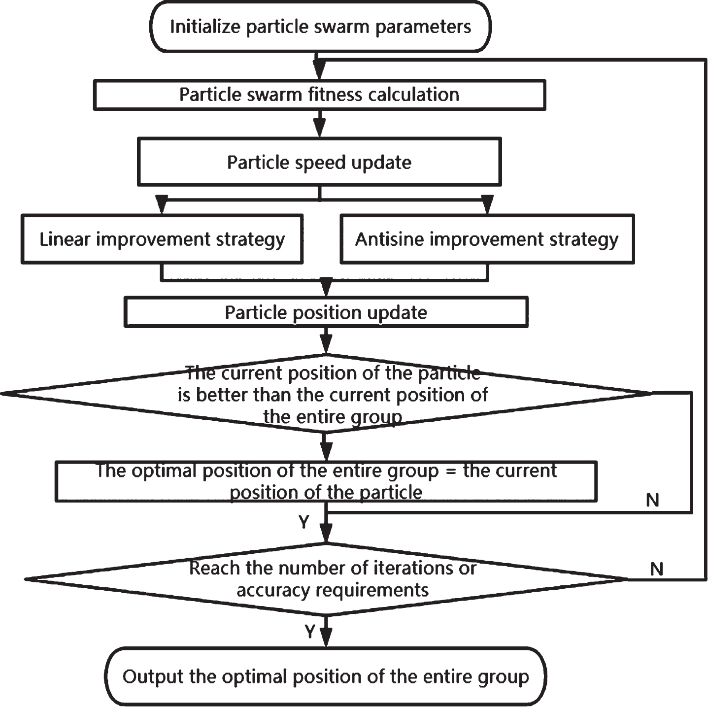
DSPSO algorithm flow chart.

4 Proposed fault diagnosis method (DSPSOBP)

The swarm intelligence of particle swarm algorithm determines that it can optimize the BP neural network. There are two main optimization methods: one method is to optimize the weight and threshold; the other method is to optimize the network structure. Network structure optimization is more complicated than network weight optimization and threshold optimization, and the change of network structure will affect the change of PSO algorithm solution space dimension, which will become more difficult to implement. In addition, it will also affect the rate of convergence during operation. Therefore, this paper chooses the BP network method that can optimize the network connection weight and threshold at the same time.

The Double Strategy Particle Swarm Optimization algorithm established in the previous chapter is used to optimize the BP neural network and optimize the weight and threshold of BP neural network, so as to make BP neural network have better performance and better participate in the process of rolling bearing fault diagnosis. This method is Double Strategy Particle Swarm Optimization BP neural network (DSPSOBP). The process of this method is as follows:

Step1: Initialization work. In the initialization work, it is mainly divided into two steps: the first step is to determine the structure of the BP neural network, that is, the number of layers and the number of nodes in each layer; the second step is to determine the parameters, the number of particles, inertia weight, speed, Parameters such as position, maximum number of iterations and acceleration constant are initialized;

Step2: Evaluation work. Select the mean square error as the evaluation standard, calculate the fitness value of the particle, and set the global optimal value to the current value, then the extreme value corresponding to the particle is the optimal value of the BP neural network in the next iteration, and the iteration starts;

Step3: Extreme value update work. After calculating the fitness value of each particle, compare the fitness value with the current value of the particle. If the fitness value of the particle has a better performance than the current value, it will be set to the current value and the extreme value will be updated; If the best extreme value of all particles has better performance than the global extreme value, it will be set to the current value and the global extreme value will be updated;

Step4: Inspection work. After optimizing the weights and thresholds, the BP neural network continues to train, and the weights and thresholds are adjusted through the iterative process of the BP neural network. If the MSE meets the desired index, the optimized weights and thresholds are set as the optimal Solution; otherwise, return to the evaluation work and continue to iterate until the conditions for stopping the iteration are met.

The framework of DSPSOBP method is shown in Fig. 3.

Fig. 3

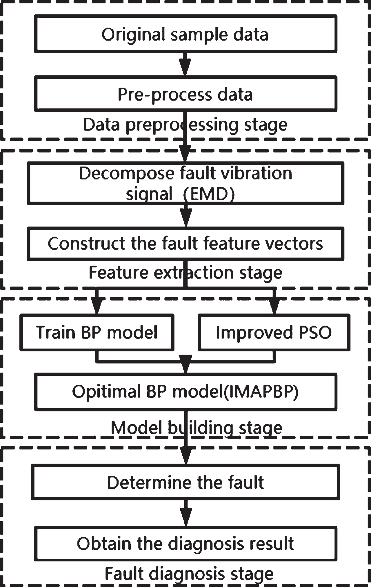
DSPSOBP flow chart.

5 Bearing fault diagnosis experiment

This section mainly uses experiments to verify the effectiveness and accuracy of the diagnostic method (DSPSOBP). The experimental data used comes from Case Western Reserve University [23]. The 6205-2RS JEM SKF deep groove ball bearing is employed in the experiment. In this bearing, the internal diameter is 25mm, the external diameter is 52mm and thickness is 15mm. The method used in the experiment is the electric spark method. The motor load is 0. Then sample the data,and the data of three fault states (inner ring, outer ring, rolling element) are collected. The sampled original vibration signal is divided into 640 data samples. The number of samples of the vibration signal in the three fault states is all 180, and the number of samples of the vibration signal in the normal state is 100.

The experiment uses the EMD method to decompose the three kinds of fault vibration signals. The IMF component is selected according to the correlation principle. The correlation principle is to calculate the relationship between each IMF component and the original signal according to the correlation coefficient, so as to select the IMF component. The threshold is set to one tenth of the maximum value of the correlation coefficient series. The calculation results of correlation coefficient are shown in Table 1. According to the calculation result sequence of correlation coefficient, the first eight IMF components can be extracted.And respectively calculate the energy of the first eight IMF components and the instantaneous amplitude of the bearing under different conditions. The energy of instantaneous amplitude is calculated and used as the input failure feature vector of DSPSOBP method. The fault feature vector is shown in Table 2, and the empirical mode decomposition diagram is shown in Fig. 4. Due to space constraints, only part of the sample is given. The obtained feature vectors of bearings in different states are randomly divided into training samples and test samples. The number of training samples under the three fault states is 144 and the number of test samples is 36. The number of training samples under normal conditions is 80 and the number of test samples is 20. Training samples are used to build fault diagnosis models, and test samples are used to test fault diagnosis models.

Fig. 4

Empirical mode decomposition diagram.

Table 1

Fault feature vector table

IMF component	IMF1	IMF2	IMF3	IMF4	IMF5	IMF6	IMF7	IMF8	IMF9
Correlation	1.8230	1.2569	1.0295	0.9846	0.8555	0.6421	0.3338	0.1985	0.0028
coefficient

Table 2

Fault feature vector table

Working state	Samples	The instantaneous amplitude energy
		features of IMF components
		E1	E2	E3	E4	E5	E6	E7	E8
Rolling element fault	1	0.732	0.632	0.246	0.152	0.032	0.002	0.002	0.001
	2	0.741	0.594	0.265	0.113	0.024	0.006	0.003	0.002
	3	0.776	0.561	0.278	0.106	0.026	0.005	0.001	0.001
Inner-race fault	1	0.962	0.298	0.105	0.062	0.015	0.003	0.003	0.000
	2	0.932	0.258	0.106	0.061	0.016	0.005	0.001	0.000
	3	0.941	0.352	0.109	0.064	0.015	0.008	0.002	0.002
Outer-race fault	1	0.745	0.667	0.104	0.026	0.006	0.002	0.001	0.001
	2	0.753	0.697	0.103	0.023	0.005	0.003	0.003	0.000
	3	0.652	0.722	0.105	0.022	0.003	0.001	0.008	0.000
Normal	1	0.536	0.708	0.205	0.232	0.326	0.062	0.001	0.005
	2	0.545	0.716	0.204	0.245	0.386	0.051	0.006	0.007
	3	0.537	0.732	0.195	0.263	0.346	0.021	0.001	0.001

Table 3

Comparison chart of fault diagnosis result

Working state	Diagnosis correctness rate (%)
	EMD-SVM	EMD-ELM	BP	PSO-BP	DSPSOBP
Rolling element fault	81.33%	77.04%	90.05%	93.46%	95.66%
Inner-race fault	86.89%	82.15%	89.07%	93.58%	96.38%
Outer-race fault	96.44%	94.85%	88.99%	93.27%	99.84%
Normal	90.47%	86.62%	91.23%	95.68%	100%

Next, the comparison of the experimental results was carried out. The BP and PSO-BP methods were compared with the DSPSOBP method and compared with other documents. The comparison of the diagnosis results is shown in Table 3 and Fig. 5. Some comparative data are from the literature [22]. The environment followed is: Inter CPU 2.30GHz, 8.0GB RAM, Matlab2018b, Windows 10 operating system.

Fig. 5

Fault diagnosis result diagram.

It can be found from Table 2 and Fig. 5: In the comparison of the three methods of BP method, PSO-BP method and DSPSOBP,we found that the results of the experiment are gradually developing in a good direction. No matter which state, the accuracy of fault diagnosis is gradually improving. And achieve the relatively best diagnosis result in the DSPSOBP method. At the same time, through comparison with other documents, we found that the improved algorithm has a greater improvement than other algorithms. Therefore, the DSPSOBP method is effective and can effectively diagnose bearing faults.

6 Conclusions

This paper mainly optimizes the BP neural network used in the field of rolling bearing fault diagnosis. Firstly, this paper adds the signal analysis and processing process, namely EMD decomposition process, to the basic model of BP neural network fault diagnosis. Secondly, this paper proposes the Dual Strategy Particle Swarm Optimization method (DSPSO), and uses this method to optimize the BP neural network, and establishes the Dual Strategy Particle Swarm Optimization BP neural network (DSPSOBP). Experiments show that the BP neural network based on DSPSO has stronger advantages than the basic model of BP neural network fault diagnosis. Experiments show the effectiveness of the optimization method and the effectiveness of DSPSO in BP neural network optimization.

Footnotes

Acknowledgments

This work has been supported by National Natural Science Foundation of China (No. 52175379).

References

Lian cheng , Ma

, Zhang

, et al., Research on Fault Diagnosis System of Crusher Based on BP Neural Network, The 32nd China Control and Decision Conference, 2020, 672–677.

, Yao

, Wang

et al., Multiscale local features learning based on BP neural network for rolling bearing intelligent fault diagnosis, Measurement 153 (2019), 107419.

Sun

, Xu

, Wang

et al., Anovel bearing fault diagnosis method based on principal component analysis and BP neural network, 2019 14th IEEE International Conference on Electronic Measurement & Instruments (ICEMI), IEEE, 2019, 1125–1131.

Lin Shuiquan

, Time-domain fault diagnosis method based on rolling machinery rolling bearings, Automation Technology and Application 39(302(08)) (2020), 5–9+39.

Zhang

, Li

, Yang

et al., Bearing Fault Diagnosis Based on BP Neural Network and Transfer Learning[J], Journal of Physics: Conference Series 1881(2) 022084. (4pp).

Qian Zhiyuan , , Genetic algorithm optimized BP neural network port crane fault diagnosis, Machinery Manufacturing and Automation 48(01) (2019), 178–181.

, Li

and Zhao

, Study on A Fault Diagnosis Method ofRolling Element Bearing Based on Improved ACOand SVM Model, International Journal of Future GenerationCommunication and Networking 9(3) (2016), 167–18.

Deng

, Yao

, Zhao

et al., A novel intelligent diagnosis method using optimalLS-SVM with improved PSO algorithm, Soft Computing 23(7) (2019), 2445–2462.

Wen Zhou , Xue Meigui , Lu Feiyan , Fault diagnosis method of sliding bearing of sealing device based on MEA-BP neural network, Light Industry Machinery 38 ;No.165(03)) (2020), 83–87.

10.

Xiao

, Zhang

, Wen

, et al., Fault Diagnosis Based on BP Neural Network Optimized by Beetle Algorithm[J], Chinese Journal of Mechanical Engineering 34(1) (2021).

11.

Guo Wenqiang , She Jinlong , Zhang Baorong , et al., Neural network bearing fault diagnosis based on PSO and GSA, 279–282, Computer Simulation 035(003) (2018), 279–282,302.

12.

Feng Yufang , Lu Houqing , Yin Hong , et al., Research on fault diagnosis model based on BP neural network, Computer Engineering and Applications 55(06) (2019), 30–36.

13.

Wang Yuwei , Wang Hongjun , Han Qiushi , et al., Rolling bearing fault identification based on wavelet packet and IGA-BP neural network, Machine Tool & Hydraulics 2019(17).

14.

Ma Chao , Wang Shaohong , Xu Xiaoli , et al., Intelligent diagnosis method of rolling bearing fault based on CSBP, Journal of Electronic Measurement and Instrument 33(12) (2019), ;No.22864–69.

15.

Cui Pengyu , Wang Zeyong , Qiu Chunrong , et al., Rolling bearing fault diagnosis method based on IBA optimized BP neural network, Electronic Measurement Technology 42(12) (2019);No.32039–42.

16.

Zhang Ning , Wei Xiuye , Guo Xiaoyong , et al., Research on bearing fault diagnosis based on improved fish school algorithm to optimize neural network, Bearing(05) (2019);No.47449–53.

17.

Zhang

et al., An Improved Simultaneous Fault Diagnosis Method based on Cohesion Evaluation and BP-MLL for Rotating Machinery, 2020 IEEE 29th International Symposium on Industrial Electronics (ISIE) IEEE, 2020.

18.

Liu Junfeng , Dong Baoying , Yu Xiang , et al., Fault diagnosis method of rolling bearing based on fsc-mpe and BP neural network [J], China Ship Research 16(6) (2021), 8.

19.

Xu Zifei , Yue Minnan , Li Chun , Fault diagnosis of rotating machinery based on manifold learning and neural network [J], Thermal Power Engineering 35(6) (2020), 9.

20.

Wang Fengtao , Deng Gang , Wang Hongtao , et al., Rolling bearing fault diagnosis method based on EMD and ssae [J], Journal of Vibration Engineering 32(2) (2019), 9.

21.

Zhang Jian , Zhang Ziyang , Qi Xuemei , et al., Rolling bearing fault diagnosis based on EMD and vpmcd [J], Mechanical Design 2019(S02) (2019), 4.

22.

Wentao , Mao , Jianliang , et al., Bearing fault diagnosis with auto-encoder extreme learning machine: A comparative study[J], Proceedings of the Institution of Mechanical Engineers, Part C: Journal of Mechanical Engineering Science 231(8) (2016).

23.

, https://engineering.case.edu/bearingdatacenter/download-data-file.