Image processing based fault classification in power systems with classical and intelligent techniques

Abstract

This paper is devoted to develop interest of power system engineers in learning basic concepts of image processing and consequently using deep networks to solve problems of complex power system networks. To this end, we study fault classification in a power system through automation of equal area (EAC) criterion. By considering EAC graphs as images and using classical image processing techniques, we successfully distinguish between different transient conditions including sudden change of input power as well as short circuit at the sending end and middle points of a single and double circuit transmission lines. In addition to classification, some parameters are also determined from EAC images such as initial rotor angle, clearing angle, and maximum rotor angle. Further, the use of deep networks is introduced to perform the same task of fault classification and a comparison is drawn with multilayer perceptron neural networks. Developed algorithms are tested in MATLAB as well as Pytorch environments.

Keywords

Engineering education power system equal area criterion image processing deep neural networks MATLAB pytorch

1 Introduction

Classification of faults in power systems is extensively studied topic. The detection and classification of these faults can lead to high-performance power systems. Literature in this area is dominated by computational intelligence methods and hybrid versions of different signal processing and soft computing techniques are shown to be promising in the detection and classification of different faults. For instance, in [1], Fourier series is utilized in conjunction with fuzzy logic to classify five transient conditions including swell, surge, sag, normal and outage. This algorithm is computationally effective as it uses only two inputs and ten rules to achieve the classification. The two inputs namely normalized peak amplitude and its derivative are extracted through Fourier series and passed to the fuzzy decision block. In [2], wavelet transform is used in place of Fourier to extract coefficients at different levels of resolution and a vector is formed from these coefficients based on their energy contents. This vector is then fed to a group of nine learning vector quantization neural networks to classify nine transient conditions. In [3], use of S-transform is investigated to extract features from power signals. It is pointed out that S-transform is preferable as compared to wavelet transform as latter may not capture important frequency components leading to limited performance. Using most significant contour of time-frequency data and signal magnitudes, fourteen rules are designed for fuzzy logic decision block to classify eight transient events. An interesting way of extracting features using S-transform is reported in [4] where area under the curve of Gaussian windows is used along with fuzzy logic to classify power system faults. In [5], hyperbolic S-transform is introduced and its coefficients are determined using power spectrum theorem. These coefficients are then used to classify the transients in power transmission networks through back propagation neural networks. The combination of wavelet transform and neural networks is reported in [6] where fundamental harmonics are obtained through former and passed to latter for classifying faults. In [7], radial basis function neural network is used without any pre-processing of input signals to classify faults and method is reported to perform better than back propagation networks. The use of deep neural networks for fault classification is reported in [8]. Here, input signals are filtered using Hilbert-Huang transform and an image is formed using time-frequency information of filtered signals. The transformed images are fed to convolutional neural networks for the purpose of classifying faults in distribution networks.

The above literature reveals a paradigm shift to deep neural networks where images are formed in some way to classify the transients. Thus, it is need of hour to equip power system engineers with techniques of image processing to better utilize deep networks in the field of power engineering. Thus, this paper is aimed to develop interest of power system engineers for using image processing based algorithms to solve problems of complex power networks. To this end, we consider EAC diagrams and utilize image processing technology to classify different transient conditions. Here, the use of classical image processing techniques is shown to achieve the classification at first stage. This involves the use of filtering operation and pixels-connectivity concepts. Through these classical operations, some parameters are extracted from EAC images which are then used to classify the transients. Next, the use of deep networks is presented in classifying the same faults and results are compared with multilayer perceptron networks. To test these algorithms, MATLAB and Pytorch programming environments are employed. To the best of authors’ knowledge, this study is unique in developing interest of power system engineers to learn image processing and deep networks and can be included as laboratory module for the course on power system stability.

This paper is arranged as: Section 2 covers the basics of EAC. Section 3 presents fault classification using classical image processing techniques. Section 4 encapsulates fault classification using deep learning. Finally, conclusions are drawn in Section 5.

2 Overview of equal area criterion

The equal area criterion can be used for a quick estimate of stability. It is a simple graphical method for concluding the transient stability. This method is only valid for a one-machine system or a two-machine system. It is an interesting method in the sense that it provides physical insight to the dynamic behavior of the machine. The basis of the method is the swing equation describing the relation between rotor angle (δ), input mechanical power (P_m) and generated electrical power (P_e): $M \frac{d^{2} δ}{d t^{2}} = P_{m} - P_{e}$ (1)

Integrating (1) with unity inertia constant (M), we compute the area under power-delta curve as: $A = \int_{δ_{0}}^{δ} (P_{m} - P_{e}) d δ$ (2)

For stability, the area under the graph of accelerating power versus δ must be zero for some value of δ, i.e., the positive (accelerating) area under the graph must be equal to the negative (decelerating) area. δ₀ is the initial steady-state operating point. At this point, the input power to the machine is equal to the developed power. If a fault occurs in a system, δbegins to increase, and the system will become unstable if δbecomes very large. There is a critical angle δ_c before which the fault must be cleared if the system is to remain stable and the equal area criterion is to be satisfied. δ_max is the power angle to which the rotor can swing before losing synchronism. We consider four different cases here, shown in Fig. 1.

2.1 Sudden change in input power

Fig.1

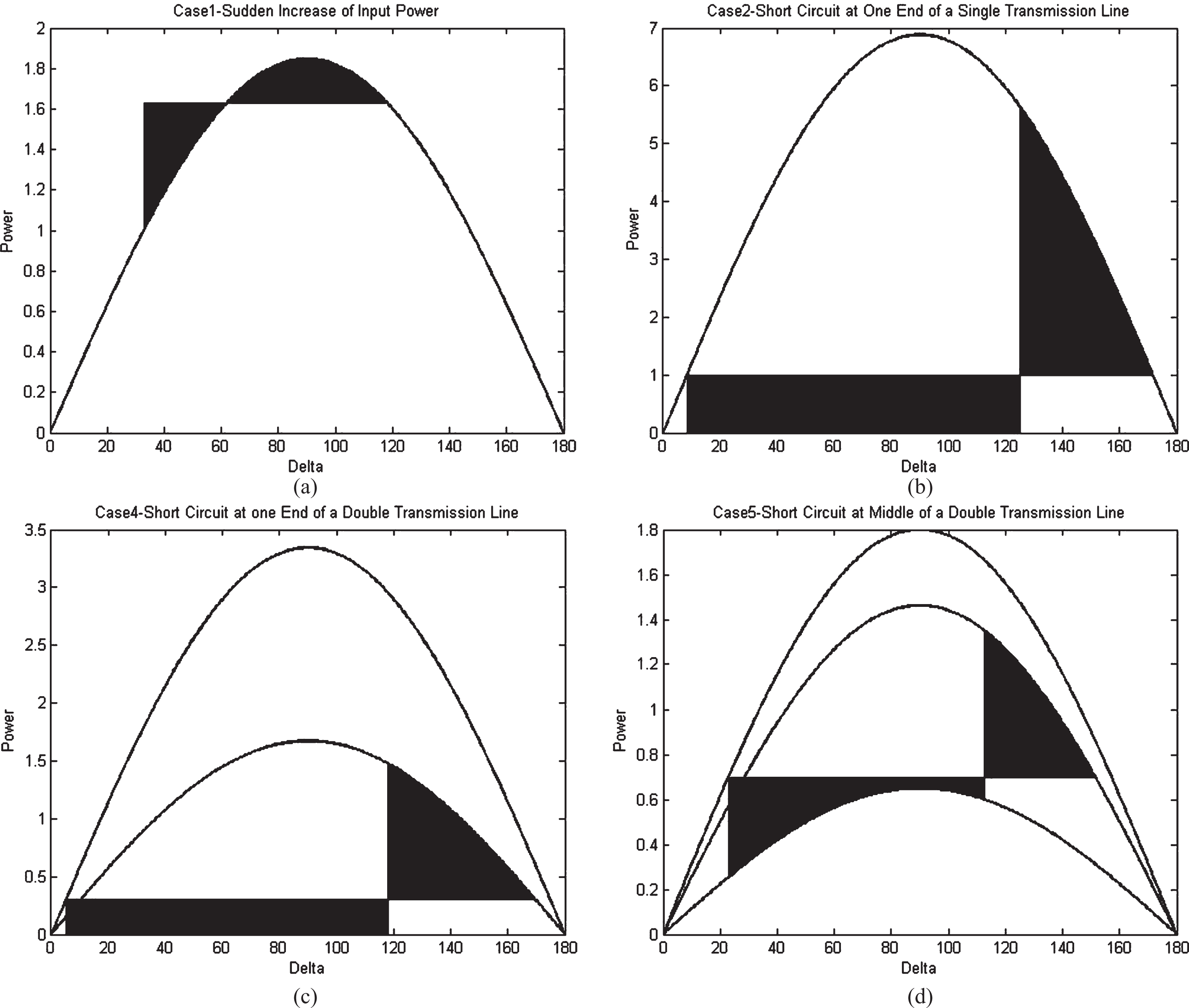
Different transient conditions in a simple power system (a) Sudden change in input power (b) Short circuit at one end of single transmission line (c) Short circuit at one end of double circuit transmission line (d) Short circuit at middle of double circuit transmission line.

When input power is suddenly increased from P_m0 to P_m1, we are interested to see the maximum swing angle of the rotor. This can be computed by equating accelerating and decelerating areas as (Fig. 1a): $\int_{δ_{0}}^{δ_{1}} (P_{m 1} - P_{max} sin δ) d δ = \int_{δ_{1}}^{δ_{2}} (P_{max} sin δ - P_{m 1}) d δ$ (3) $sin δ_{1} (δ_{2} - δ_{0}) + cos δ_{2} - cos δ_{0} = 0$ (4)

When δ₁ → δ_c, then maximum permissible rotor swing is achieved i.e. δ₂ → δ_max which happens with a maximum allowable power step-change.

2.2 Short circuit at one end of a single transmission line

During this condition, electric power transfer remains blocked till fault is cleared. This should happen before the critical rotor angle is reached. This can be determined by equating the two areas (Fig. 1b) as: $\int_{δ_{0}}^{δ_{1}} P_{m} d δ = \int_{δ_{1}}^{δ_{2}} (P_{max} sin δ - P_{m}) d δ$ (5) $sin δ_{0} (δ_{2} - δ_{0}) + cos δ_{2} - cos δ_{1} = 0$ (6)

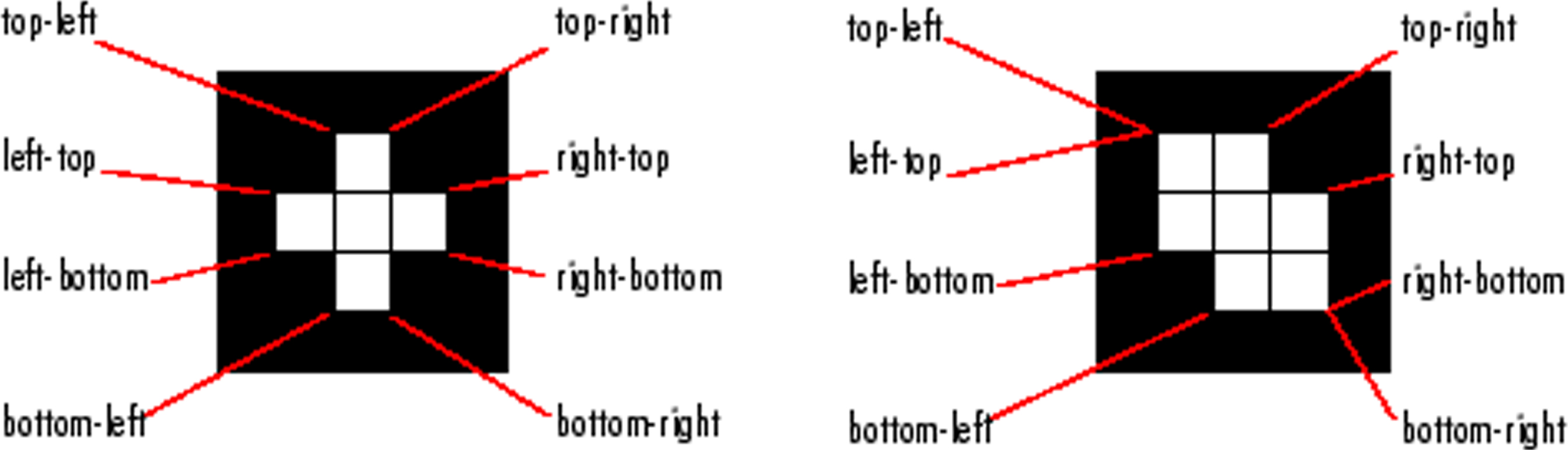
When δ₁ → δ_c, we have δ₂ → π - δ₀. This leads to determining critical angle and critical time using (6) and (1) as: $δ_{c} = {cos}^{- 1} ((π - 2 δ_{0}) sin δ_{0} - cos δ_{0})$ (7) $t_{c} = \sqrt{\frac{2 H (δ_{c} - δ_{0})}{π f P_{m}}}$ (8)

Fig.2

An illustration of extreme points of connected region [9].

2.3 Short circuit at one end of a double transmission line

In this case, electric power transfer is also interrupted during the short circuit fault. Power is restored to a lower level after the line is removed from the system (Fig. 1c). Calculation of rotor angles is the same as in Case 2.2.

2.4 Short circuit at middle of a double transmission line

In this case, electric power transfer continues during the fault (P_eB) at a lower level than normal (P_eA). After the faulty line is removed, power is restored to a higher level (P_eC) which is still lower than the normal case (P_eA > P_eC > P_eB) (Fig. 1d). Fault clearing angle (δ₁) can be determined by equating the colored areas: $\int_{δ_{0}}^{δ_{1}} (P_{m} - P_{eB max} sin δ) d δ = \int_{δ_{1}}^{δ_{2}} (P_{eC max} sin δ - P_{m}) d δ$ (9)

3 Fault classification using classical image processing techniques

In this section, an algorithm is presented to classify different transient cases as described in section 2 by using classical image processing operations.

3.1 Algorithm design

The proposed algorithm is structured into three functions namely Non_Colored_Region_Processing, Colored_Region_Processing, and Classification_EAC. First function is responsible for processing the non-colored portion of the image. This function is intended to locate the boundaries of EAC image which is achieved by measuring the extreme points of the region having maximum area. These extreme points are illustrated in Fig. 2. Using the extreme points, horizontal and vertical distances are also computed. These distances along with bottom left point of largest-area region (origin of graph) will be used by second function.

Fig.3

Block diagram of classical image processing based fault classification.

Second function is developed to process the colored portion of the graph which refers to the accelerating and decelerating areas. In order to detect the colored regions, filtering operation is first performed on EAC image which removes the boundaries such as axis. The remaining objects in the filtered image are scanned and objects having an area greater than certain threshold are retained. Extreme points of perimeters of such objects are determined which are further processed to determine rotor angles and power levels, which are also the outputs of second function. Note that lengths of horizontal and vertical segments are scaled to 180 and 10, respectively.

Third function calculates four parameters based on the information returned from the second function. These parameters are then used to distinguish between different transient conditions as described in Section 2. In this way, fault classification is achieved using classical image processing techniques. Block diagram of the proposed algorithm is shown in Fig. 3. The detailed implementation of the proposed algorithm is also included in this section.

Non_Colored_Region_Processing(EAC_image)

BW ←Convert input image to black and white scale

Y ←Fill holes in the inverse of BW image

STATS_NC ← Measure region properties of Y

For i ← 1 to length (STATS_NC)

If STATS1 (i). Area > 200

Top_Left ←

Pixel value at top right point of the region

Bottom_Left ←

Pixel value at bottom left point

Bottom_Right ←

Pixel value at bottom right point

Total_Horizontal_Distance ←

Norm (Bottom_left – Bottom_right)

Total_Vertical_Distance ←

Norm(Bottom_Left – Top_left)

End If

End For

Return (Total_Horizontal_Distance,

Total_Vertical_Distance, Bottom_Left)

Colored_Region_Processing(EAC_Image, THD, TVD, BL)

Set dummy ← 0, temp ← 0, temp1 ← 0

Set distance ← 0, distance1 ← 0

Total_Horizontal_Distance←THD

Total_Vertical_Distance←TVD

Bottom_Left←BL

BW ←Convert input image to black and white scale

Y ←Filter BW image with a 3x3 matrix with all 1’s

Z ←Find the boundary pixels in inverted image, Y

STATS_CD ← Measure region properties of Z

For k← 1 to length (STATS_CD)

If STATS_CD (k).Area>100

Top_Left1 ← Pixel value at top left point

Left_Bottom←Pixel value at left bottom point

Right_Top← Pixel value at right top point

If dummy = 0

temp ← Point on vertical axis in front of

Top_Left1

temp1 ← Point on vertical axis in front

of Left_Bottom

distance ← Norm (Bottom_Left – temp)

distance1←Norm (Bottom_Left – temp1)

Set dummy1← 1

Power (dummy1) ← $\frac{distance \times 10}{Total_Vertical_Distance}$

Power (dummy1 + 1) ← $\frac{distance 1 \times 10}{Total_Vertical_Distance}$

End If

If dummy = 1

temp ← Point on vertical axis in front

of Right_Top

distance ← Norm (Bottom_Left– temp)

Power (dummy1 + 2) ← $\frac{distance \times 10}{Total_Vertical_Distance}$

End If

Temp ← Point on horizontal axis in front of

Left_Bottom

temp1 ← Point on horizontal axis in front

of Right_Top

dummy ← dummy+1

distance ← Norm (Bottom_Left – temp)

distance1 ← Norm(Bottom_Left – temp1)

Delta (dummy) ← $\frac{distance \times 180}{Total_Horizontal_Distance}$

Delta (dummy+1) ← $\frac{distance 1 \times 180}{Total_Horizontal_Distance}$

End If

End For

Return (Delta(1), Delta(2), Delta(3), Power(1),

Power(2), Power(3))

Fig.4

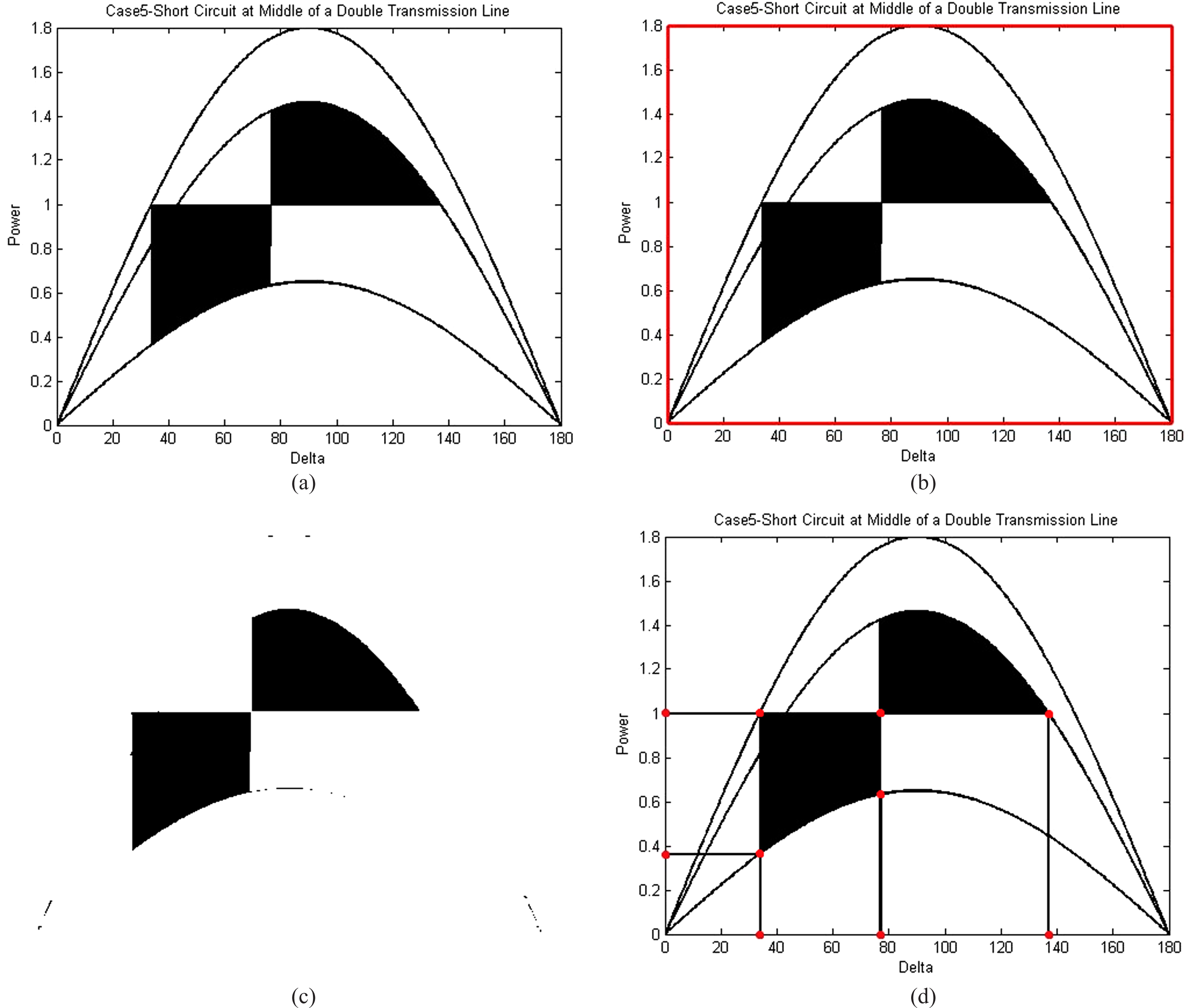
Intermediate results of proposed algorithm (a) Original image (b) Non-colored region detection (c) Filtering operation (d) Rotor angles and power level detection.

Classification_EAC (Delta1, Delta2, Delta3, Power1, Power2, Power3)

δ _ 0← ← Delta1

δ_c ← Delta2

δ_max ← Delta3

error ← 0.5

case_type ← 0

P1 $\leftarrow \frac{Power 1}{sin (δ_{0})}$

P2 $\leftarrow \frac{Power 2}{sin (δ_{0})}$

P3 $\leftarrow \frac{Power 1}{sin (δ_{c})}$

P4 $\leftarrow \frac{Power 3}{sin (δ_{max})}$

If (abs (P3 – P4)< =error)

Then case_type ←1

End if

If (abs (P1 – P4)< =error) and P2< =error)

Then case_type ←2

End if

If (abs (P2 – P3)< =error) and (abs(P3 – P4)< =

error) and (P1 > P4) and (P1< =10 + error))

Then case_type ←3 End if

If (abs (P1 – P4)>error) and (P2 > error) and

(P2 < P4))

Then case_type ←4

End If

Return (case_type)

3.2 Results

Fig.5

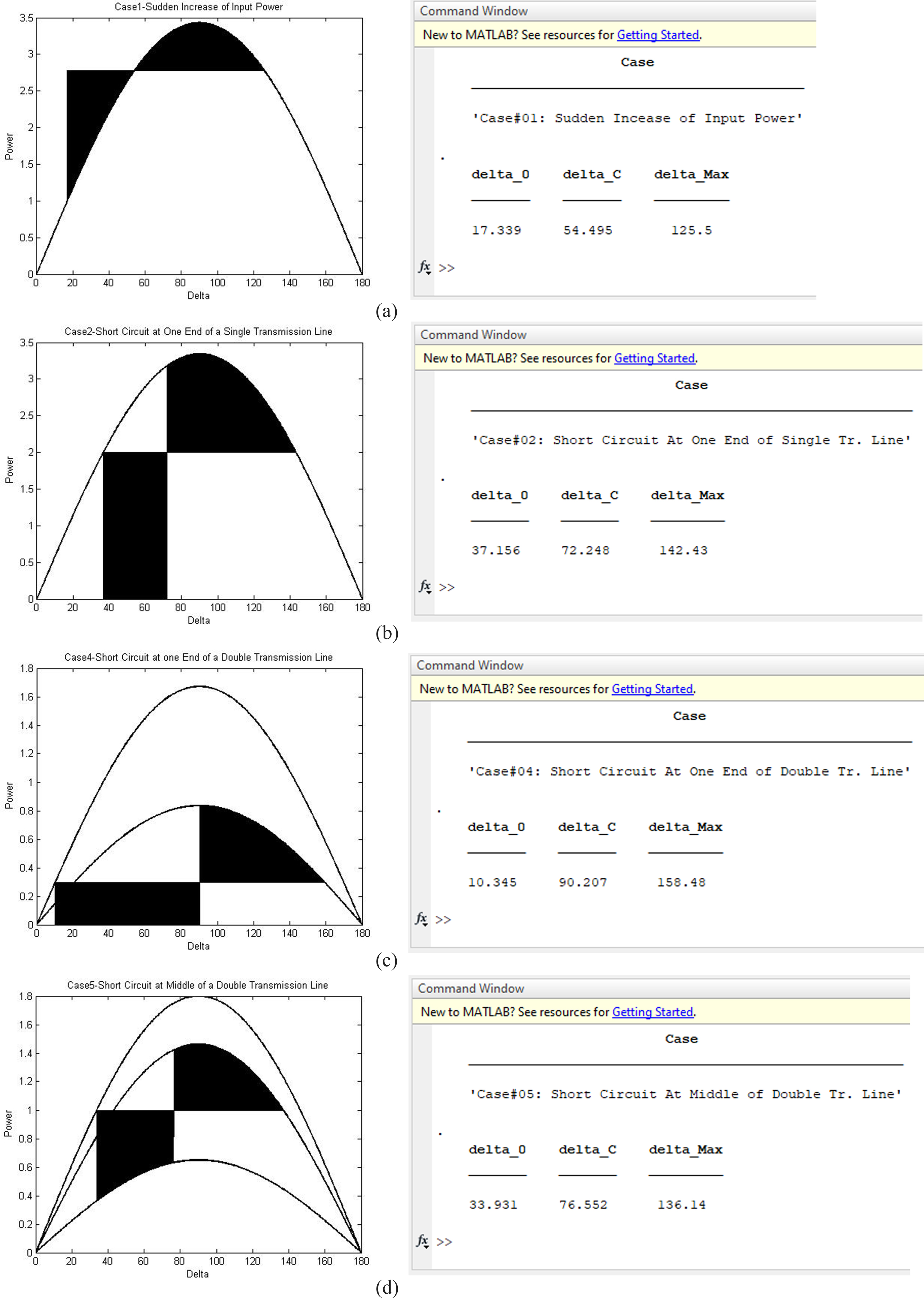
Detection and measurement of transient states through proposed algorithm (a) Sudden change in input power (b) Short circuit at one end of single transmission line (c) Short circuit at one end of double circuit transmission line (d) Short circuit at middle of double circuit transmission line.

The proposed algorithm is implemented in MATLAB programming environment and various experiments are performed to check the validity of the proposal. As an example, we show some intermediate steps while considering the case of short circuit in middle of double transmission line. Original image, shown in Fig. 4a, is processed by using first function and the detected region is highlighted in red, as shown in Fig. 4b. Original image is also processed using second function and the results of filtering and colored-boundaries detection are shown in Fig. 4c and d, respectively.

A total of sixteen EAC images (four for each case) are checked through the proposed algorithm and algorithm has remained successful in classifying the transient conditions and rotor angles are correctly determined as well. The results for different cases are included in Fig. 5.

Fig.6

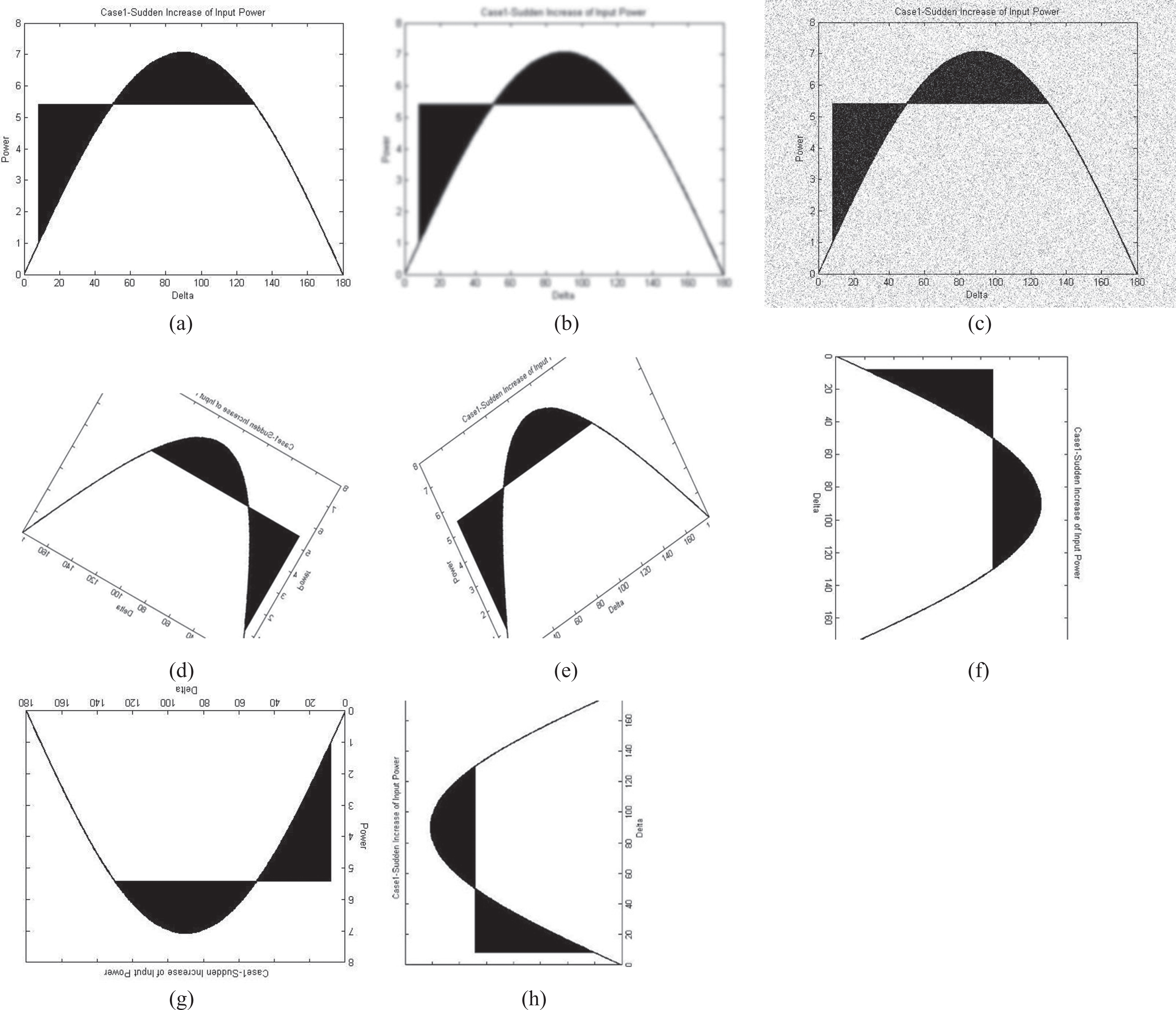
Data augmentation (a) Original image (b) Gaussian blur (c) Random noise (d) Rotated by 30deg (e) Horizontally flipped (f) Rotated by 90deg (g) Rotated by 180deg (h) Rotated by 270deg.

4 Fault classification using intelligent image processing techniques

In this section, neural networks are used to classify the faults. A simple multilayer perceptron is initially used to distinguish between the transient conditions occurring in power systems. Then, convolutional neural network is tried for the same task. The working pipeline for both the approaches consists of two parts: data augmentation and classification.

4.1 Data augmentation

A deep learning task requires plentiful data to train the network so that it can distinguish between diverse class labels. In our case, we don’t have enough data, so to cater this problem and increase the amount of data, new data is synthesized from the existing images. For this purpose, we have used the data augmentation technique which applies several procedures and generate slightly modified copies of the original data; thereby increasing the dataset. Different methods are used to generate synthetic data which include rotation, cropping, padding etc. In our case, to extend the dataset, each original image is manipulated by:

applying Gaussian Blur

adding noise

rotating by different angles; 90, 180, and 270 degrees

rotating by 30 degrees and flipping horizontally

In this way, every original image is augmented to generate seven further images, as shown in Fig. 6.

4.2 Classification

4.2.1 Classification using multilayer perceptron network

A multilayer perceptron (MLP) is a feed forward artificial neural network which operates on a supervised learning technique called back propagation. Its architecture is built upon at least three layers of nodes: an input layer, a hidden layer and an output layer. Each output from a neuron passes through an activation function which helps in normalizing its output. Either it’s a classification or prediction problem; where inputs are assigned a class or label, or regression prediction problems; where a real-valued quantity is predicted given a set of inputs; both can be solved easily through MLP. They can be used on image data, text data, time series data and other types of data.

A neural network is built by using a set of neurons. Each hidden layer consists of numerous of them and they are further connected to every neuron in the subsequent layer. The neurons hold some weight and bias for every input. The input is multiplied by its weight and then summed together to return an output. Further, this output is passed through an activation function which helps to normalize it to a specific range, thus making the network learn.

In this section, we present the proposed MLP architecture for the detection of transient conditions, captured through EAC images. It contains 2 hidden layers. The learning rate is set to 0.0003 and CrossEntropyLoss is used to calculate loss of our network. In CrossEntropyLoss, NLLLoss (negative log likelihood loss) and LogSoftmax are combined into one single class.

For MLP, input data needs to be passed as a vector. So for this reason, we converted our input image of size (224*244) to a vector of size 50176 and passed it as input to the model.

As shown in Fig. 7, input vector of size 50176 is passed to the first hidden layer of size 1000. Its output is further passed on to the subsequent hidden layer of size 500, whose output is finally passed to the output layer of size 4, representing each of our class.

Fig.7

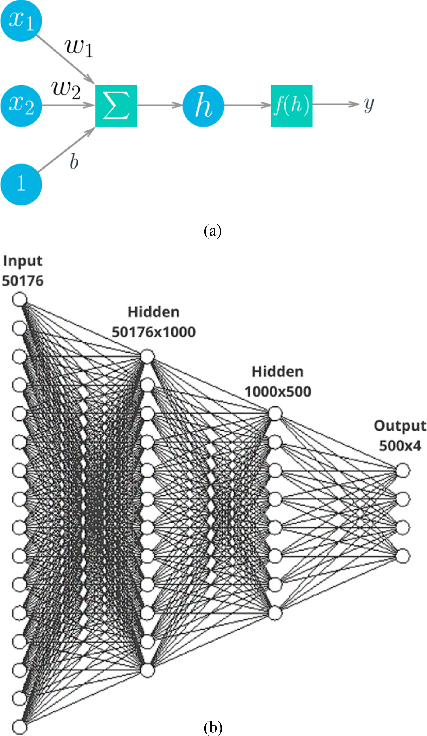
Neural network architecture (a) A single neuron (b) Proposed architecture for fault classification.

4.2.2 Classification using convolutional neural network

A convolutional neural network (CNN) is a type of deep neural network which is mostly used for diverse image classification tasks. It doesn’t require much pre-processing as compared to other classification algorithms and consists of convolutional layer, pooling layer and fully connected layer, which are explained below:

1) Convolutional Layer: A convolutional neural network can maintain spatial information. It looks at an image as a matrix and analyzes a group of pixels at a time, unlike multilayer perceptron which takes in a vector of image pixels. The spatial information of image is maintained using convolutional layers.

A convolutional layer applies series of different convolution filters to the input image which extracts different features from the image like edges or colors, which distinguish different objects in the image. The result from this layer is passed to a subsequent convolutional layer which further applies more convolutional filters to it. The innovation of convolutional neural networks is the ability to automatically learn a large number of filters which can extract meaningful information such as finding patterns.

Fig.8

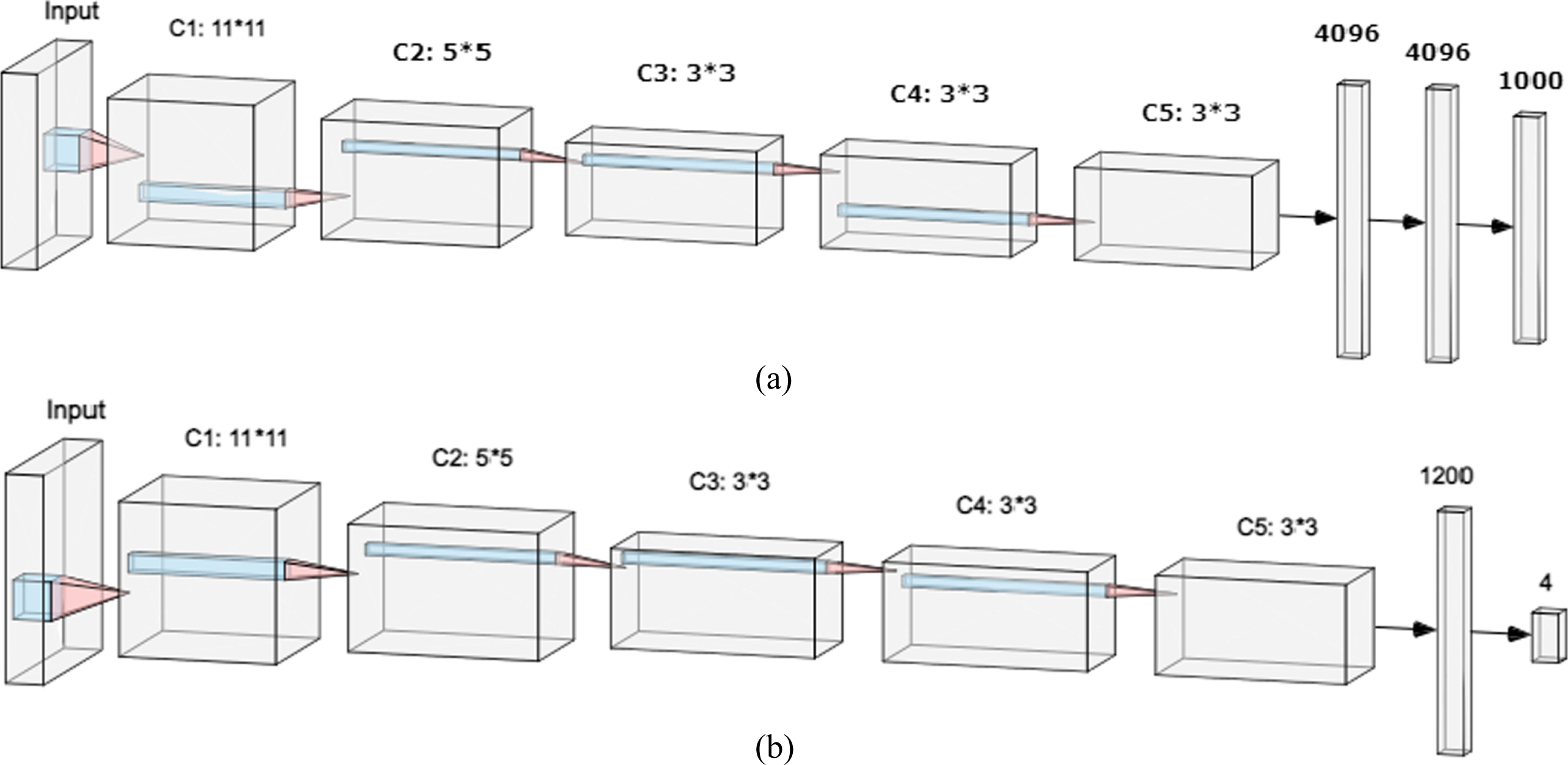
Convolutional neural network (a) AlexNet (b) Modified AlexNet.

2) Pooling Layer: The results from a series of convolutional layers are passed on to the pooling layer. A convolutional layer can apply several convolutional filters due to which the dimension of convolutional layer can get quite large. It implies that it will require more computational power as well. So, to reduce the dimensionality, pooling layers are employed. There are two type of pooling operations; max pooling and average pooling. It is also helpful for extracting features which are rotational and positional invariant.

3) Fully Connected Layer: A fully connected layer has all it neurons connected to the all the neurons in the previous layer. This layer is a traditional artificial neural network which performs classification based on the features extracted by the previous layers.

For classification of transient conditions occurring in power systems using convolutional neural network, we are using transfer learning. Transfer learning is a technique that reuses knowledge of a pre-trained model on a new problem. It means that what’s learned from another dataset on another problem will be transferred to your dataset. There are two ways in which transfer learning can be used.

Through parametric changes in some layers of a trained CNN

By using trained CNN, for calculating feature maps of new types of data

Fig.9

Loss curves (a) MLP (b) CNN.

We are only utilizing the feature maps extracted from AlexNet as images in our dataset and hose in ImageNet dataset differ from each other, but we can still use basic image features like edges and shapes which are extracted by this network. As illustrated in Fig. 8a, AlexNet contains 5 convolution layers and 3 fully connected layers at the end. The last fully connected layer is of size 1000 which represents each of the class in ImageNet dataset.

As we are using only feature maps extracted from AlexNet, we are using 5 convolution layers of AlexNet and one fully connected layer of size 1200, as shown in Fig. 8b. Input image of size 224*224 is passed to the network and output from the convolution layers is of size 256*6*6. For the optimization step, we are using Average stochastic gradient descent and the learning rate is set to 0.001. CrossEntropyLoss is used to calculate loss of our network. In CrossEntropyLoss, NLLLoss (negative log likelihood loss) and LogSoftmax are combined into one single class.

4.3 Results

Both neural networks, MLP and CNN are implemented using Pytorch and the model is trained and tested on google colab. As a preprocessing step, pixels of image to be given as input to these networks are normalized between range [0, 1]. In case of MLP, there’s an additional step of converting the image to grayscale before normalizing. Furthermore, size of image is reduced to 224x224 which helps the networks to learn faster and gives better results also.

To evaluate the performance of our models, k-fold validation is used. The models are split into 5 folds with 80% training set and 20% test set. For CNN, each split is trained for 100 epochs after which accuracy is calculated, whereas in the case of MLP, 30 epochs are used. The results established from k-fold evaluation of both MLP and CNN are shown in Table 1 and 2, respectively. For MLP, we have achieved an accuracy of 87% while a much higher accuracy of 99% is obtained using CNN approach. Moreover, loss curve for one of the folds as calculated using CrossEntropyLoss, is included in Fig. 9.

Table 1
MLP performance

Fold Class Correct Prediction Accuracy

Fold-1 Case-1 (6/7) 85%

Case-2 (5/6) 83%

Case-3 (7/7) 100%

Case-4 (6/6) 100%

Total Accuracy (Fold-1) (24/26) 92%

Fold-2 Case-1 (6/7) 85%

Case-2 (5/6) 83%

Case-3 (7/7) 100%

Case-4 (6/6) 100%

Total Accuracy (Fold-2) (24/26) 92%

Fold-3 Case-1 (6/6) 100%

Case-2 (6/7) 85%

Case-3 (7/7) 100%

Case-4 (6/6) 100%

Total Accuracy (Fold-3) (25/26) 96%

Fold-4 Case-1 (6/6) 100%

Case-2 (4/7) 57%

Case-3 (4/6) 66%

Case-4 (6/6) 100%

Total Accuracy (Fold-4) (20/25) 80%

Fold-5 Case-1 (6/6) 100%

Case-2 (1/6) 16%

Case-3 (6/7) 85%

Case-4 (6/6) 100%

Total Accuracy (Fold-5) (24/26) 76%

Total Accuracy (112/128) 87%

Fold	Class	Correct Prediction	Accuracy
Fold-1	Case-1	(6/7)	85%
	Case-2	(5/6)	83%
	Case-3	(7/7)	100%
	Case-4	(6/6)	100%
Total Accuracy (Fold-1)	(24/26)	92%
Fold-2	Case-1	(6/7)	85%
	Case-2	(5/6)	83%
	Case-3	(7/7)	100%
	Case-4	(6/6)	100%
Total Accuracy (Fold-2)	(24/26)	92%
Fold-3	Case-1	(6/6)	100%
	Case-2	(6/7)	85%
	Case-3	(7/7)	100%
	Case-4	(6/6)	100%
Total Accuracy (Fold-3)	(25/26)	96%
Fold-4	Case-1	(6/6)	100%
	Case-2	(4/7)	57%
	Case-3	(4/6)	66%
	Case-4	(6/6)	100%
Total Accuracy (Fold-4)	(20/25)	80%
Fold-5	Case-1	(6/6)	100%
	Case-2	(1/6)	16%
	Case-3	(6/7)	85%
	Case-4	(6/6)	100%
Total Accuracy (Fold-5)	(24/26)	76%
Total Accuracy	(112/128)	87%

Table 2

CNN performance

Fold	Class	Correct Prediction	Accuracy
Fold-1	Case-1	(7/7)	100%
	Case-2	(6/6)	100%
	Case-3	(7/7)	100%
	Case-4	(6/6)	100%
Total Accuracy (Fold-1)		(26/26)	100%
Fold-2	Case-1	(7/7)	100%
	Case-2	(6/6)	100%
	Case-3	(6/6)	100%
	Case-4	(7/7)	100%
Total Accuracy (Fold-2)		(26/26)	100%
Fold-3	Case-1	(6/6)	100%
	Case-2	(7/7)	100%
	Case-3	(6/6)	100%
	Case-4	(7/7)	100%
Total Accuracy (Fold-3)		(26/26)	100%
Fold-4	Case-1	(6/6)	100%
	Case-2	(7/7)	100%
	Case-3	(5/6)	83%
	Case-4	(6/6)	100%
Total Accuracy (Fold-4)		(24/25)	96%
Fold-5	Case-1	(6/6)	100%
	Case-2	(6/6)	100%
	Case-3	(7/7)	100%
	Case-4	(6/6)	100%
Total Accuracy (Fold-5)		(26/26)	100%
Total Accuracy		(127/128)	99%

5 Conclusions

In this paper, we have presented an image processing based fault classification scheme to motivate power engineers to learn and utilize two dimensional signals processing for solving complex power system problems. The use of both classical as well as intelligent image processing techniques is presented to classify transient conditions by considering EAC graphs as images. The proposed work can also be included as a laboratory module for power system stability course.

References

Dash

P.K.

, Mishra

, Salama

M.M.A.

and Liew

A.C.

, Classification of power system disturbances using a fuzzy expert system and a Fourier linear combiner, IEEE Transactions on Power Delivery 15 (2000), 472–477.

Borras

, Castilla

, Moreno

and Montano

J.C.

, Wavelet and neural structure: a new tool for diagnostic of power system disturbances, IEEE Transactions on Industry Applications 37 (2001), 184–190.

Chilukuri

M.V.

and Dash

P.K.

, Multiresolution S-transform-based fuzzy recognition system for power quality events, IEEE Transactions on Power Delivery 19 (2004), 323–329.

Srikanth

and Koley

, Fuzzified time-frequency method for identification and localization of power system faults, Journal of Intelligent and Fuzzy Systems, In press (2021).

Chang

H-H.

, Linh

N.V.

and Lee

W.-J.

, A novel nonintrusive fault identification for power transmission networks using power–spectrum–based hyperbolic S-transform-Part-I: fault classification, IEEE Transactions on Industry Applications 54 (2018), 5700–5710.

Soleymani

, Bastam

and Mozafari

, Fault diagnosis of transmission system based on wavelet transform and neural network, Journal of Intelligent and Fuzzy Systems 25 (2013), 271–277.

Lin

W.-M.

, Yang

C.-D.

, Lin

J.-H.

and Tsay

M.-T.

, A fault classification method by RBF neural network with OLS learning procedure, IEEE Transactions on Industry Applications 16 (2001), 473–477.

Guo

M.-F.

, Yang

N.-C.

and Chen

W.-F.

, Deep learning based fault classification using Hilbert-Huang transform and convolutional neural network in power distribution systems, IEEE Sensors Journal 19 (2019), 6905–6913.

Image processing toolbox, MATLAB.