A hybrid approach using CNN and active contour model for automated segmentation of macular edema

Abstract

Macula is the part of retina responsible for sharp and clear vision. Macular edema is caused by the accumulation of intraretinal fluid (IRF) in the macula, which is further distinguished by the compromised integrity of the blood-retinal barrier, particularly evident in the retinal vasculature. This results in swelling, that may lead to vision impairment and is the dominant sign of several ocular diseases, including age-related macular degeneration, diabetic retinopathy, etc. Quantitative analysis of the fluid regions in macular edema helps in ascertaining the severity as well as the response to treatment of the diseases. Optical coherence tomography (OCT) is a major tool used by ophthalmologists for visualizing edema. The prevalent practice for diagnosing and treating macular edema involves measuring Central Retinal Thickness (CRT). Segmenting the IRF in OCT images offers the potential for a more accurate and better quantification of macular edema. This paper proposes a novel method combining convolutional neural network (CNN) and active contour model for segmenting the IRF to ascertain the severity of macular edema. The IRF region is initially segmented using an encoder-decoder architecture. Contour evolution is then performed on this segmented image to demarcate the IRF boundaries. The advantage of the method is that it does not require precisely labeled images for training the CNN. A comparison of the experimental results with models employing CNN alone and with other state-of-the art methods demonstrates the superior performance and consistency of the proposed method.

Keywords

edema segmentation convolutional neural network active contour model

1 Introduction

The macula, located near the retina’s central region, plays a crucial role in facilitating central vision. Diseases affecting the retina can cause the accumulation of fluids in the macula and result in macular edema. This causes swelling and vision impairment. Diabetes also can lead to macular edema by causing injury to the blood vessels within the retina, resulting in the accumulation of intraretinal fluid (IRF). This condition is called diabetic macular edema (DME), marked by the breakdown of the blood-retinal barrier within the retinal blood vessels [1]. Swelling also occurs due to damaged pigment epithelium, which causes the accumulation of subretinal fluid (SRF), though its occurrence is relatively infrequent. Assessing the quantity of IRF and SRF can provide valuable insights into the diseases.

Early detection of the retinal diseases is particularly important to prevent loss of vision. Also, understanding the severity of the disease is crucial for planning image guided therapy. Images obtained from OCT serve as an important tool in the visualization of edema [2]. The advancements in OCT imaging technology, along with its versatility in assessing various diseases, make it suitable for large screening scenarios. Inbuilt automated segmentation techniques are currently unavailable in commonly used OCT devices. As a result, thickness measurements from these scans are done manually. Obtaining quantitative information on anatomy and abnormality via manual delineation is often strenuous and time consuming.

Currently, quantitative information about the edema is obtained through measurement of central retinal thickness (CRT) [3]. In CRT measurement, the inner limiting membrane (ILM) and RPE layers are segmented to obtain the thickness of the retina. However, CRT is not capable of giving an exact measure of the size of the IRF as it also includes the thickness of the retinal layers [4]. Achieving a more precise quantification of macular edema by directly segmenting the IRF in OCT images can provide detailed information about the extent and location of fluid accumulation [5]. This information is crucial for monitoring disease progression, assessing treatment efficacy, and guiding therapeutic interventions. A comparison of CRT measurement and IRF segmentation is shown in Fig. 1. From the figure, it can be seen that IRF segmentation gives an exact measure of edema thickness while CRT gives a measure of retinal thickness including the layers.

Fig. 1

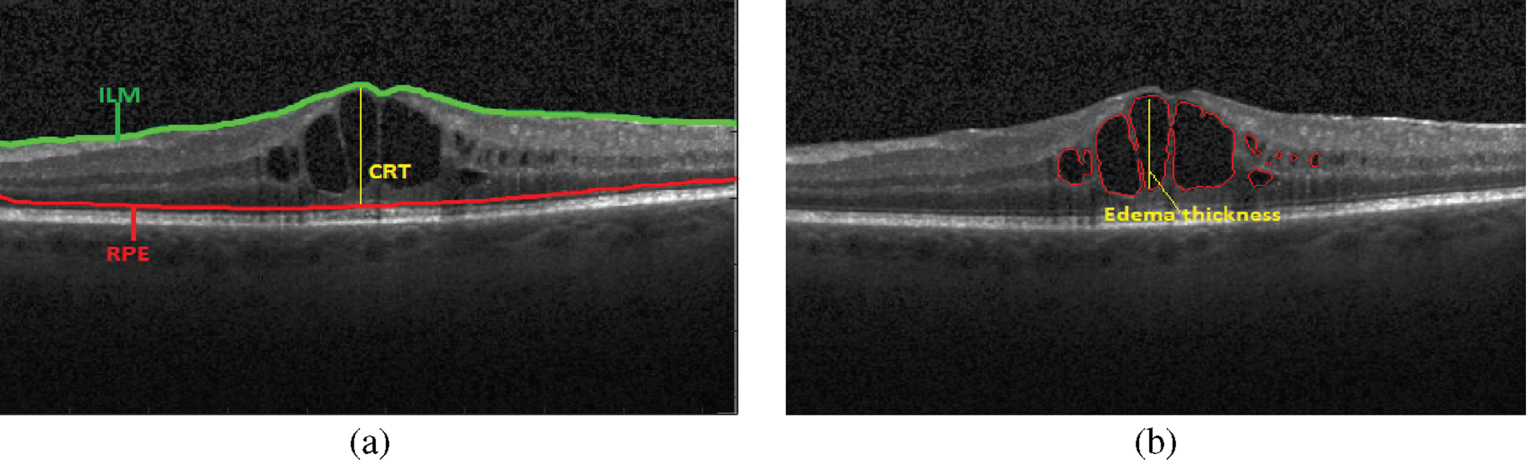
Comparison of CRT and IRF measurements a) CRT measurement b) IRF measurement.

Segmenting intraretinal fluid (IRF) in OCT images poses significant challenges that include morphological changes resulting from pathologies with high variability in image appearance, inherent speckle in OCT images and the difficulty in designing algorithms that can function consistently across images obtained from different machines. Since the majority of the methods using handcrafted features rely on the quality of OCT images, the results may vary with image quality [6]. Deep learning-based methods proved successful in such cases for reliable segmentation of DME. In this paper we propose a hybrid method combining CNN and active contour for automatic segmentation of macular edema. The contribution of the work is in proposing a hybrid model for segmenting the IRF and ascertaining it’s severity that alleviates the complexities of training the CNN and the initialisation sensitivity of the active contour model.

The rest of the paper is organized in the following manner: Section 2 reviews some of the important works in edema segmentation. While Section 3 outlines the methodology, Section 4 delves into a discussion of results emanating from the method and comparison with state of the art methods. The paper is concluded in Section 5.

2 Related work

A review of some of the key studies employing deep learning for the segmentation of IRF in OCT images is presented here. In the work of Lee et al. [7], a modified version of the UNet architecture, with 18 convolutional layers are employed. While deep learning technique shows promising outcomes in precise segmentation and automated quantification of IRF, it is worth to note that the results might lack generalizability. Additionally, to ensure satisfactory performance, training should encompass a diverse range of pathologies. In [8], Tennakoon et al. proposed a CNN for edema segmentation. The method successfully segmented retinal fluids at the voxel level based on the predictions. Lu et al. [9] proposed a multi-class retinal fluid segmentation model using deep learning. The method successfully segmented the fluid regions and results were comparable with ground truth. In [10], Gao et al. proposed a model using improved UNet architecture. The method was validated on public dataset and experiments demonstrated that the proposed method enhances precision in detecting diverse edema across multiple regions.

In [11], Jonathan et al. implements deep convolutional neural networks with extremely limited datasets for macular edema segmentation. CNN architecture in this application setting demonstrate the ability to attain performance levels close to human expertise on unseen test images without the need for extensive training examples. Junjie Hu [12] uses deep neural networks (DNNs) in conjunction with atrous spatial pyramid pooling (ASPP) for automatic segmentation of SRF and Retinal pigment epithelial detachment (PED) lesions. Experimental findings demonstrate that the integration of DNNs with ASPP yields superior segmentation accuracy compared to state-of-the-art methods. In [13], Gordón et al. introduced a novel Fully Convolutional Network design that employs spatial and channel attention gates across various scales to achieve precise segmentation. A weighted loss strategy also is incorporated to address class imbalance.

Though CNN-based methods produced promising results, the segmentation accuracy for the method discussed above depends on labelling of the images also. Labelling of IRF is a tedious task and in many cases it is not possible to label the IRF precisely. Also, the labelling of IRF for training purposes is a time-consuming job and needs expertise. To alleviate the difficulties of training the CNN, a combination of CNN followed by an active contour model is proposed here for IRF segmentation. The advantage of this method is that it requires only a rough labelling of IRF region and precise labelling as done in methods based on CNN alone is not required.

3 Methodology

For segmenting the IRF and ascertaining the severity of edema, a two-step approach as shown in Fig. 2 is proposed. The first step involves training a convolutional neural network (CNN) to produce the pixel-wise labels of the IRF region and background. The CNN analyzes each pixel and classifies it as either belonging to the IRF region or the background. The input image is then multiplied with the output from CNN to extract the IRF region alone and eliminating the background as shown in Fig. 3.

Fig. 2

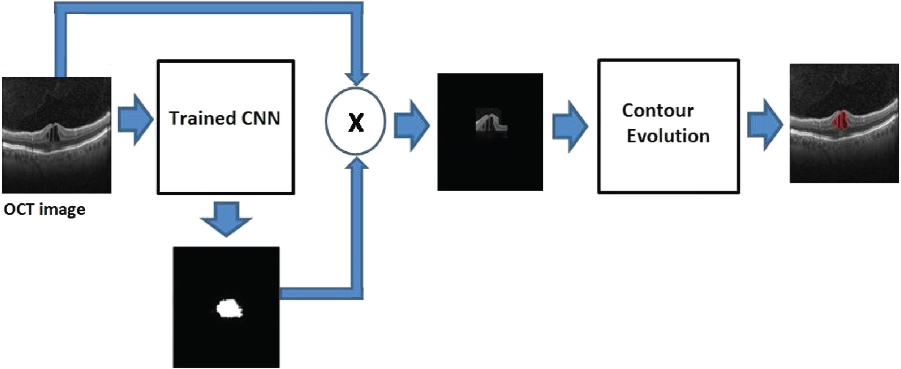
Two-step approach for IRF segmentation.

Fig. 3

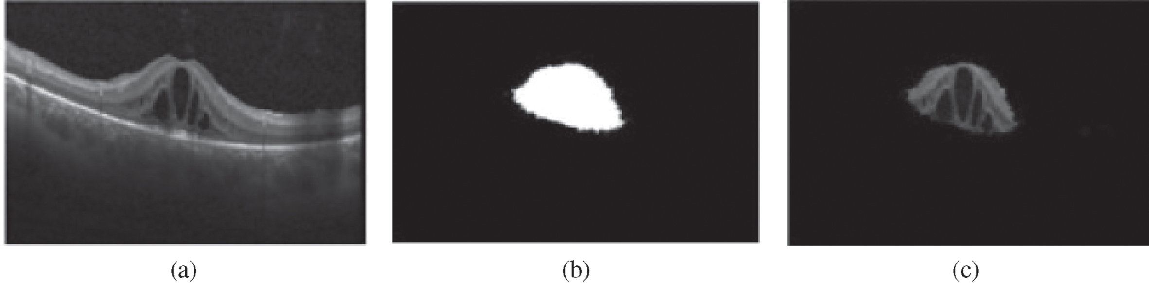
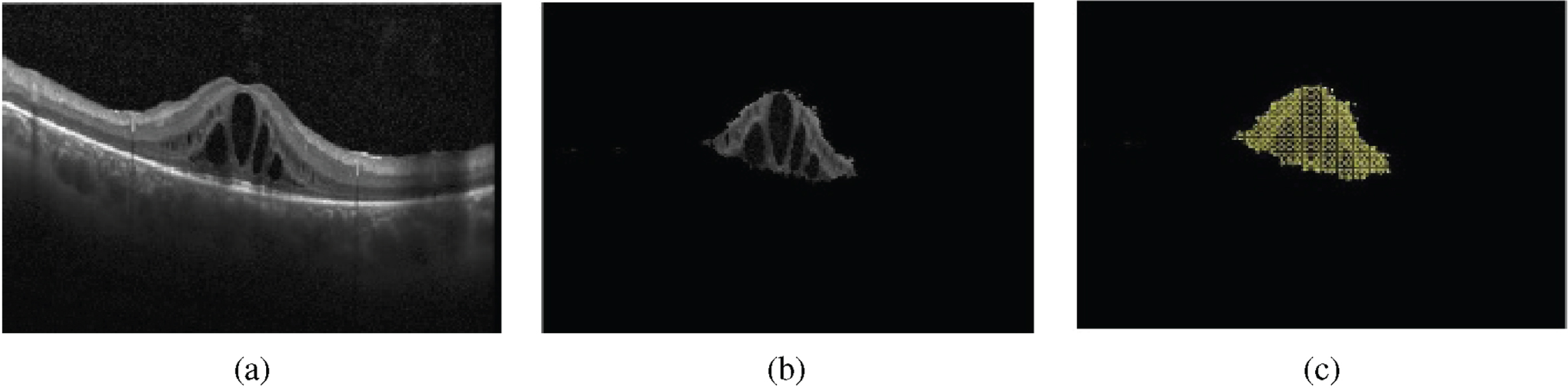
Image extraction a) OCT image b) CNN output c) Extracted image.

In the second step, Chan-Vese contour evolution is performed on the extracted image to segment the IRF boundaries. The initial contour for this segmentation is defined over the extracted image using checkerboard initialization [14]. This helps active contour to segment multiple fluid-filled regions, if present. The maximum height of the segmented IRF is then taken as the edema thickness.

3.1 CNN for segmentation

To perform segmentation of IRF, we adopted an encoder-decoder architecture, which used the underlying architecture of SegNet, introduced in [15]. The SegNet framework consists of an encoder network, a decoder network, and a pixel wise classification layer. Instead of using fully connected layers at the end of the encoder, the decision has been made to retain higher-resolution feature maps at the last encoder output. This approach is common in encoder-decoder architectures for tasks like image segmentation. It helps preserve spatial information and reduces the number of parameters.

The encoder consists of 13 convolutional layers which are well-suited for capturing spatial hierarchies and local patterns in data, making them effective in image-related tasks. The decoder also has 13 layers, with each layer corresponding to a layer in the encoder. The decoder’s role is typically to upsample the features and generate a spatially aligned output. The final decoder output is followed by a softmax classifier, which produces class probabilities independently for each pixel. Low-resolution feature maps are generated at the encoder using a combination of convolution, ReLu, and batch normalization, followed by maxpooling layers. The decoder recovers high-resolution feature maps through upsampling. Also, maxpooling indices from the corresponding encoder layer helps in recovering spatial information. The final softmax layer produces pixel-wise class probabilities.

In the training process, the cross-entropy loss between the predicted class and the actual class is back propagated for every pixel, leading to the update of both encoder and decoder weights. The pixel-wise cross-entropy (CE) loss evaluates the distance from the output probabilities to the true values of each pixel and is given by: $CE = - \frac{1}{W} \sum_{n = 1}^{W} l_{n} log (Q_{n}) + (1 - l_{n}) log (1 - Q_{n})$ (1) where W represents the data points, Q _n is the softmax probability for the nth data point, and l _n represents the true class labels.

In the OCT images used for our experiment, the number of pixels in the background is very large compared to the IRF class. Since cross-entropy loss evaluates each pixel loss individually, the training can be dominated by the background class. So, to weigh the loss differently based on the true class, median frequency balancing [16] is used in the work. The scaling factor α is given by: $α = \frac{f_{ave}}{f}$ (2) where, f is the class frequency and f _ave is the average of all class frequencies. The final loss is then obtained as average of the sum of weighted loss over all the pixels in a mini-batch. During training, the difference between the actual class and predicted class represented by the cross entropy loss is back propagated to update the weights. To optimise the weights so as to minimise the loss function we use stochastic gradient descent (SGD) algorithm.

The CNN architecture employed for IRF segmentation is illustrated in Fig. 4. The encoder comprises a total of 13 layers of convolution. The first two layers have depths of 64 and 64, respectively, while the subsequent two layers have depths of 128 each. This pattern continues with depths of 256 in the next three layers, and finally, the last four layers have depths of 512 each. After each convolution layer, batch normalization is performed and Rectified Linear Unit (ReLU) activation function is applied to enhance the model’s stability and to introduce non-linearity. Additionally, there are five max pooling layers interspersed between these convolution layers. These pooling layers aid in reducing the spatial dimensions of the feature maps, contributing to the network’s ability to capture hierarchical features. The overall design is structured to progressively extract complex representations of the input data, culminating in a deep and hierarchically organized encoder for effective IRF segmentation.

Fig. 4

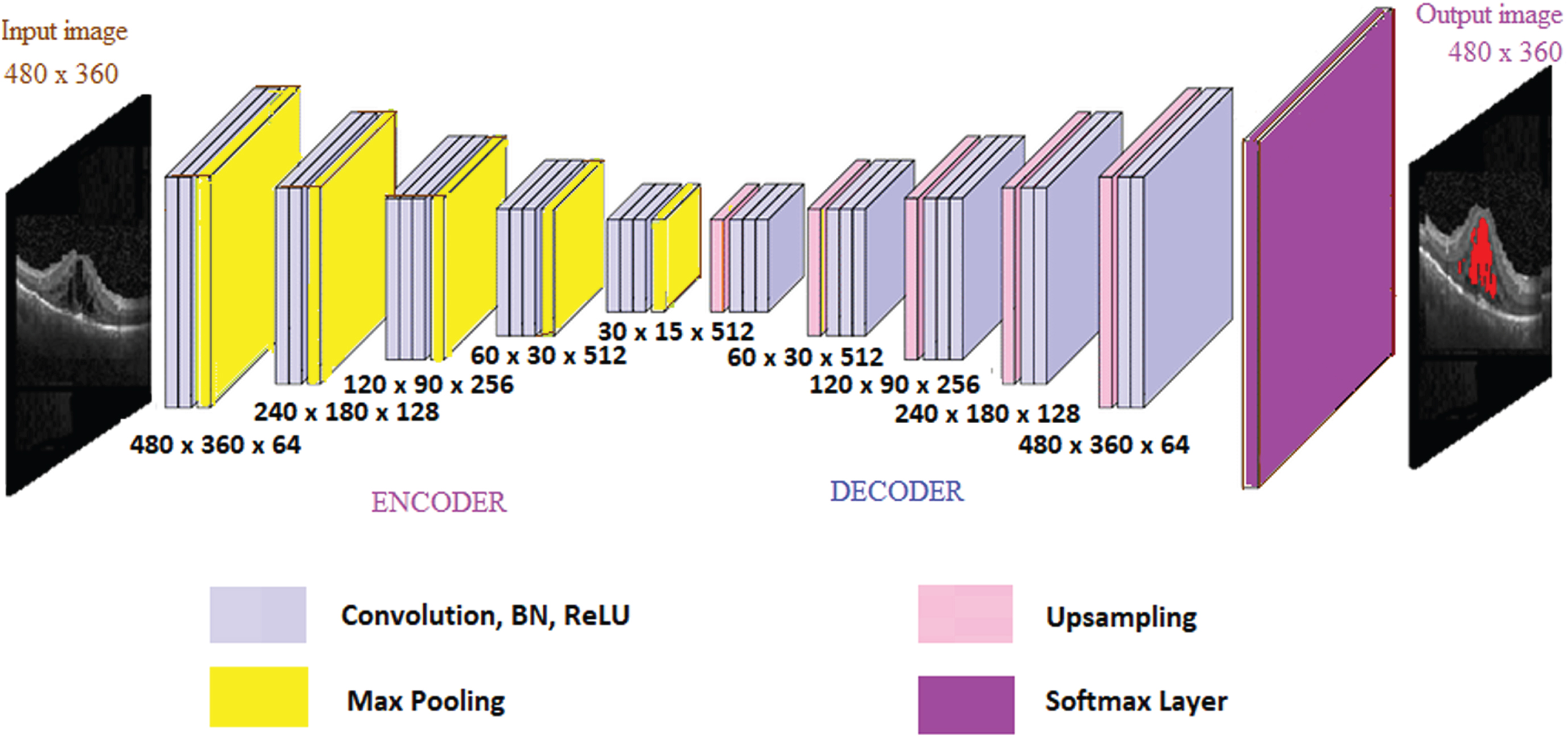
Encoder decoder architecture for IRF segmentation.

The decoder has convolution layers arranged in reverse order. A 3 × 3 kernel is used for all convolution layers. Finally, the softmax layer produces pixel-wise class labels. The pixel labels from CNN are converted into segmentation of IRF by an active contour model. When contour evolution stops, the boundaries represent IRF.

3.2 Active contour model for IRF segmentation

The proposed pipeline employs Chan Vese method [17] for effectively segmenting the IRF in OCT images. In active contour model, a curve is evolved subject to constraints from the input image. The contour detect objects in the image. Active contour model may lead to improper segmentation if the contour initialisation is not proper. To alleviate this initialization sensitivity, the contour in our work is initialized in the region derived from the output of CNN.

If I is the image in the domain Ω, the contour evolution minimises the energy function given by $\begin{array}{l} E (ψ, a_{1}, a_{2}) = μ . \int_{Ω} δ (ψ) | ▽ ψ | + λ_{1} \int_{Ω} | I - a_{1} |^{2} \\ H (ψ) d x d y + λ_{2} \int_{Ω} | I - a_{2} |^{2} (1 - H (ψ)) d x d y \end{array}$ (3)

Here, the initial contour is represented by a Lipschitz function (ψ), the Heaviside function (H) and the dirac measure (δ). a ₁, a ₂ represent the average values of the image for ψ ≥ 0 and ψ < 0 respectively. The parameters μ, λ₁, λ₂ are determined experimentally.

In the proposed model, first we extract the portion of the image where the IRF is present as depicted in Fig. 5b. The initialisation of the level set for Chan-Vese method is then performed by using a checkerboard shape as shown in Fig. 5(c)x. The initial contour for this segmentation is defined such that the extracted image is covered with a checkerboard of small contours of radius 3 pixels. Thus, the objective defined on the whole image is localized by splitting it into different sub domains. Initial contour in these domains then evolve tracking the variations and converges to local minima, which are the edges of IRF.

The tedious task of precise labelling can be avoided using this combined approach. Since the area of the extracted image is very small, contour evolution stops in lesser number of iterations capturing the local variations resulting in perfect segmentation.

Fig. 5

Contour initialisation a) OCT image b) Extracted image c) Checkerboard.

4 Experiments

4.1 Dataset

The data set used in the proposed pipeline consists of 2000 images of DME with different resolutions acquired from Kermany et al. [18]. The images were labeled under the supervision of a retinal expert and using the Image Labeler software present in Matlab. During the training process, the entire IRF region is labeled as a single class, and there is no need for precise labeling. An example of a labeled image used for training the model is illustrated in Fig. 6. An additional set of 250 images, obtained from Donghuan Lu et al. [9], has been utilized as the ground truth for testing purposes. Sample images from [9] used for testing are shown in Fig. 6(c).

Fig. 6

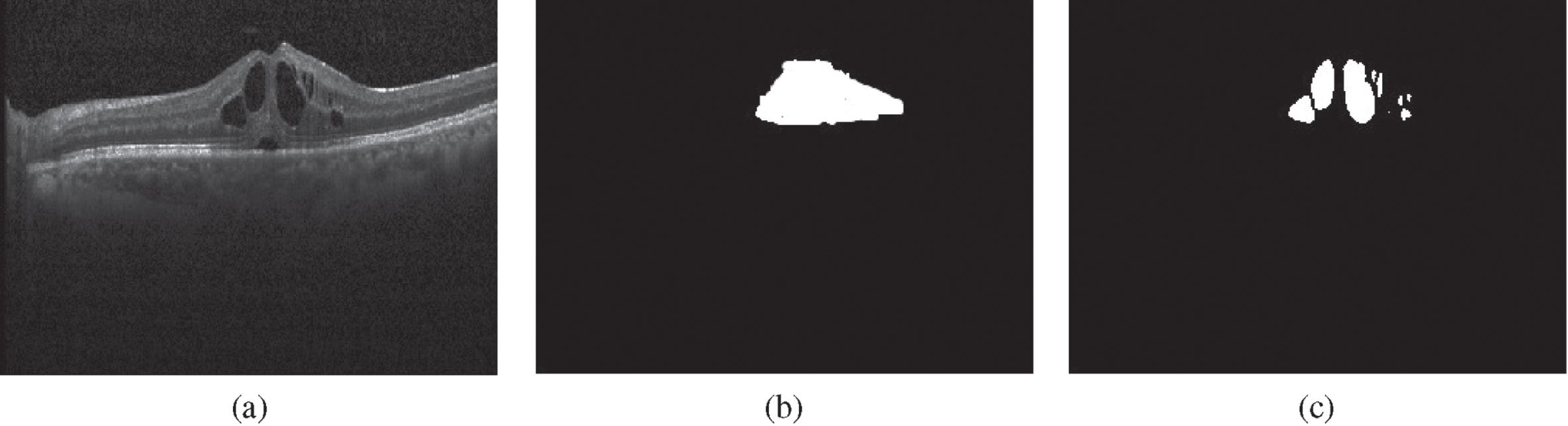
Example of labelled images a) Sample image b) Image labelled using Image Labeler and c) Labelled images from [9].

4.2 Training

The network is trained with a learning rate of 0.0001 using stochastic gradient descent with a momentum of 0.9. During testing, the network produces pixel-wise labels of the IRF region and the background. Output obtained from the CNN is used to extract the image with IRF, over which contour evolution is performed. In the Chan-Vese model, for perfect fitting of the contour around IRF, the value of μ in Equation 3 is determined experimentally as 0.001. The parameters λ₁ and λ₂ for the second and third terms, respectively in Equation 3 are set to 1.

4.3 Evaluation

For evaluating the performance of the proposed model we used Precision (Pr), Recall (Re), BF score (BF) and Dice Coefficient (D _c) to ascertain the agreement of the proposed method with ground truth. Precision, recall, and BF score are metrics employed to assess the closeness of boundaries between the ground truth and the segmented region. This closeness is quantified by considering a distance tolerance, providing a measure of how well the segmented boundaries align with those of the ground truth. The Dice coefficient serves as a metric for assessing segmentation quality, indicating the degree of similarity between the segmented region and the ground truth. The Dice coefficient is calculated as the ratio of twice the number of pixels that overlap between the segmented region and the ground truth for a specific class, and the total number of pixels encompassing both regions combined. A value of one signifies complete overlap between the two regions, while a value of zero indicates no overlap. The performance metrics are evaluated as: $\Pr = \frac{P 1}{P 1 + P 2}$ (4) $Re = \frac{P 1}{P 1 + N 2}$ (5) $BFscore = \frac{2 (\Pr) (Re)}{\Pr + Re}$ (6) where P1 is True positive, N1 is True Negative, P2 is False positive and N2 is False Negative. The Dice coefficient is formally expressed as: $D_{c} = \frac{2 x Area of overlap}{Total area}$ (7)

4.4 Results and discussion

The proposed pipeline used a hybrid approach using CNN architecture and active contour model for automated segmentation of Macular Edema. The average values of Dice coefficient, precision, recall, and BF score obtained for 250 test images using our proposed algorithm is compared with the state-of-the-art techniques are summarized in Table 1. The Table also presents the results obtained by employing a human expert for the intended task.

Table 1
Comparison of segmentation results with state-of-the-art techniques. All results are generated using the same dataset [18]

Dice BF Precision Recall

coefficient score

Our method 0.93 0.97 0.96 0.97

UNet 0.91 0.96 0.95 0.96

SegNet [19] 0.8 0.88 0.85 0.93

Method [9] 0.85 0.91 0.89 0.96

Expert Vs Ground truth 0.79 0.88 0.9 0.86

	Dice	BF	Precision	Recall
Our method	0.93	0.97	0.96	0.97
UNet	0.91	0.96	0.95	0.96
SegNet [19]	0.8	0.88	0.85	0.93
Method [9]	0.85	0.91	0.89	0.96
Expert Vs Ground truth	0.79	0.88	0.9	0.86

All the images acquired from [9] were tested using the proposed framework. The curves evolved after contour evolutions represent the boundaries of IRF. Output obtained at each stage of the process are shown in Fig. 7. The input OCT image is shown in Fig. 7a. CNN output is shown in in Fig. 7b. CNN output is multiplied with the input image to obtain the extracted image as shown in Fig. 7c. Contour evolution is then performed on this extracted image and Fig. 7d shows the result after contour evolution.

Fig. 7

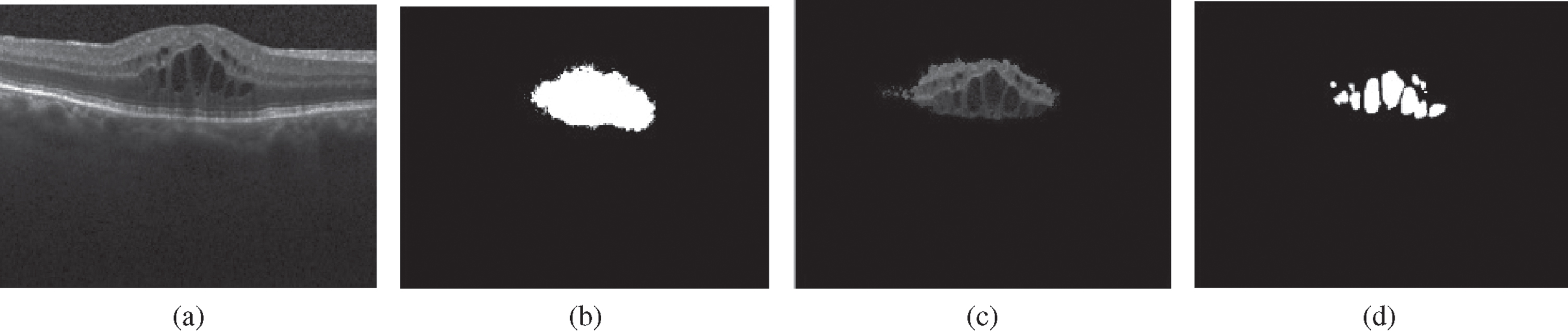
Segmentation of IRF (a) Original image (b) CNN output (c) Extracted image (d) Segmented IRF.

Segmentation results obtained using the proposed method are then compared with the ground truth. Figure 8 shows the comparison of the results with ground truth for two different images in the data set. The boundary points of segmented IRF obtained after contour evolution are marked on the input image for better visualisation and is shown in yellow color in Fig. 8c and f. The IRF boundary obtained from the ground truth is marked on the input image and is shown in green color in Fig. 8b and e.

Fig. 8

Results obtained using two different images from [9]. (a, d) Input image, (b, e) ground truth, and (c, f) output of the proposed model overlayed on the input image.

The results achieved with the combination of CNN and active contour are better than those obtained using SegNet [19], as well as with UNet and the method proposed in [9]. The segmentation results obtained using other techniques present in the literature depend on the training data set that contains wide variety of pathological images. With the proposed hybrid method, CNN segments the IRF part alone, which does not require complex training. Also, the active contour model segments the IRF by tracking local variations to find edges of the IRF, which results in perfect segmentation.

Once the IRF is segmented, the thickness of the edema is quantified. The method involves determining the maximum height of fluid accumulation within the segmented IRF regions. This measurement is taken as the thickness of the IRF, which contributes for a first-level information on the edema severity [20]. To find agreement with manual measurement, the maximum thickness obtained using the proposed method is compared with the value obtained manually.

For an image, the difference in thickness obtained between automated method and ground truth in pixels is taken as the error. Average value obtained for 250 images is represented as mean error (ME). Mean of the absolute value of the difference is the mean absolute error (MAE). Table 2 shows comparison of the results with the proposed method and other state-of-the-art techniques. Also, to find inter observer variability, ME and MAE between expert and ground truth were calculated.

Table 2

Error and absolute error in edema thickness. Figures outside the bracket represent mean of the value and that inside the bracket shows standard deviation in pixels

	ME	MAE
Our method	1.05 (2.9)	2.3 (1.65)
UNet	1.15 (3.2)	2.48 (2)
SegNet [19]	1.91(4.8)	3.7 (3.5)
Method [9]	1.21 (4)	2.6 (3.3)
Expert Vs Ground truth	2.5 (2.9)	2.95 (2.4)

As shown in Table 2, for our method, the mean error and mean absolute error are 1.05 and 2.3 pixels respectively, while those obtained with method [9] are 1.21 and 2.6. Between experts, the values obtained are 2.5 and 2.95 for the mean error and mean absolute error. This shows that the results obtained using the combination of CNN and the active contour method outperform other well-known methods, and the error is less than that with expert.

5 Conclusion

For segmentation of IRF in OCT images, a unique combination of CNN and active contour model is proposed here. In the two step approach, a CNN is trained to obtain the pixel wise labels of the IRF region. The input image is then multiplied with the output from CNN and the area containing IRF alone is extracted. Chan-Vese contour evolution is then performed on the extracted image to segment the IRF boundaries. Quantitative and qualitative results obtained using the combined method proved consistent with expert labellings. The prime advantage of the model is that it avoids the tedious task of precise labelling of IRF. Experimental results validate the reliability of the algorithm. The accurate measurement of thickness of the edema is expected to enable the ophthalmologists for exact diagnosis and better treatment of retinal diseases.

References

Marmor

M.F.

, Mechanisms of fluid accumulation in retinal edema. InMacular Edema: Conference Proceedings of the 2 nd InternationalSymposium on Macular Edema, Lausanne, 23-25 April (pp.35-45). Springer Netherlands, (2000).

Trichonas

Kaiser

P.K.

, Optical coherence tomography imagingof macular oedema, British Journal of Ophthalmology 98(Suppl 2) (2014), ii24–ii29.

Keane

P.A.

Sadda

S.R.

, Predicting visual outcomes for maculardisease using optical coherence tomography, Saudi Journal ofOphthalmology 25(2) (2011), 145–158.

Browning

D.J.

Stewart

M.W.

Lee

, Diabetic macular edema:Evidence-based management, Indian Journal of Ophthalmology 66(12) (2018), 1736.

Jintao

Minghui

Wenyu

Xianfu

Cheng

Gang

, Segmentation of diabetic macular edema in OCT retinal images, Opto-Electronic Engineering 45(7) (2018), 170605–1.

Wang

Zhang

Sun

Yao

Yan

, Detection of diabeticmacular edema in optical coherence tomography image using animproved level set algorithm, BioMed Research International 2020 (2020).

Lee

C.S.

Tyring

A.J.

Deruyter

N.P.

Rokem

Lee

A.Y.

, Deep-learning based, automated segmentation of macular edema inoptical coherence tomography, Biomedical Optics Express 8(7) (2017), 3440–3448.

Tennakoon

Gostar

A.K.

Hoseinnezhad

Bab-HadiasharRetinal

Retinal fluid segmentation in OCT images using adversarial loss based convolutional neural networks, In 2018 IEEE 15th International Symposium on Biomedical Imaging (ISBI 2018) (pp. 1436–1440). IEEE (2018).

Heisler

Lee

Ding

G.W.

Navajas

Sarunic

M.V.

Beg

M.F.

, Deep-learning based multiclass retinal fluid segmentationand detection in optical coherence tomography images using a fullyconvolutional neural network, Medical Image Analysis 54(2019), 100–110.

10.

Gao

Wang

, Automatic segmentation of macular edemain retinal OCT images using improved U-Net++, Applied Sciences 10(16) (2020), 5701.

11.

Frawley

Willcocks

C.G.

Habib

Geenen

Steel

D.H.

Obara

Segmentation of macular edema datasets with small residual 3D U-Net architectures, in 2020 IEEE 20th International Conference on Bioinformatics and Bioengineering (BIBE) (pp. 582–587). IEEE (2020).

12.

Chen

, Automated segmentation of macular edema inOCT using deep neural networks, Medical Image Analysis 55 (2019), 216–227.

13.

Cazañas-Gordón

da Silva Cruz

L.A.

, Multiscaleattention gated network (MAGNet) for retinal layer and macularcystoid edema segmentation, IEEE Access 10 (2022), 85905–85917.

14.

Getreuer

, Chan-vese segmentation, Image Processing On Line 2 (2012), 214–224.

15.

Badrinarayanan

Kendall

Cipolla

, Segnet: A deepconvolutional encoder-decoder architecture for image segmentation, IEEE transactions on Pattern Analysis and Machine Intelligence 39(12) (2017), 2481–2495.

16.

Eigen

Fergus

Predicting depth, surface normals and semantic labels with a common multi-scale convolutional architecture, in: Proceedings of the IEEE International Conference on Computer Vision (2015), 2650–2658.

17.

Chan

T.F.

Vese

L.A.

, Active contours without edges, IEEETransactions on Image Processing 10(2) (2001), 266–277.

18.

Kermany

D.S.

Goldbaum

Cai

Valentim

C.C.

Liang

Baxter

S.L.

Zhang

, Identifying medical diagnoses and treatablediseases by image-based deep learning, Cell 172(5) (2018), 1122–1131.

19.

George

Jiji

C.V.

Oct segmentation using convolutional neural network, in: 2020 IEEE 17th International Symposium on Biomedical ImagingWorkshops (ISBIWorkshops) (pp. 1–4). IEEE (2020).

20.

Nicoara

S.D.

Spectral domain optical coherence tomography in the diagnosis and monitoring of diabetic macular edema, In OCT-Applications in Ophthalmology. IntechOpen (2018).