Information structures in a multiset-valued information system with application to uncertainty measurement

Abstract

Information system (IS) is a significant model in the field of artificial intelligence. Information structure is not only a research direction in the field of granular computing (GrC), but also an important method to study an IS. A multiset-valued information system (MVIS) refers to an IS where information values are multisets. A MVIS can be seen as a model that is the result of information fusion of multiple categorical ISs. This model helps deal with missing values in the dataset. This paper studies information structures in a MVIS on the view of GrC and consider their application for uncertainty measurement (UM). First of all, some notions of multisets and probability distribution sets (PDSs) are proposed. Naturally, relationships between multisets and PDSs are researched. Then, the concept of a MVIS based on the notion of multisets is given, and the internal structure of a MVIS is revealed by an incomplete information system (IIS). Furthermore, tolerance relations in a MVIS are defined by using Hellinger distance, and tolerance classes are obtained to construct the information structures of a MVIS. Considering the association of information structures, relationships between information structures are raised from the two aspects of dependence and separation. Moreover, some properties between information structures are provided by using information distance and inclusion degree. Finally, four UMs as the applications of information structures are investigated, and comprehensive experiments on several datasets demonstrate the feasibility and superiority of the proposed measures. These results will be helpful for establishing a framework of GrC in a MVIS and studying UM.

Keywords

GrC RST Information fusion PDS MVIS Information structure UM

1 Introduction

1.1 Background and related work

There are always coexisting certain and uncertain phenomenon in the objective world. To understand the objective world, human have spontaneously developed an organized and hierarchical way of mindset of granulation. Granular computing (GrC) is a new discipline that studies mindset of granulation and its methodology. GrC [50] was first proposed by Zadeh in 1996. It can dispose large-scale complex data sets and is an important tool for data mining and knowledge representation [47].

The main goal of GrC is to deal with uncertain information and it is also a significant tool to study information systems. The major methods to study GrC are rough set theory (RST) [35, 36], fuzzy set theory [51], quotient space theory [54] and other artificial intelligence theories [18, 21].

RST [34] was proposed by Polish mathematician Pawlak in 1982, it has been a mathematical theoretical method for processing incomplete, imprecise and inconsistent information. At present, RST is successfully applied to data mining [6], machine learning [7], knowledge discovery [16, 28] and other fields. In RST, an information table is also a way of knowledge representation and that is called an IS. An IS is a database that describes the relationship between objects and attributes. The equivalence relation in an IS can be regarded as a special similarity relation between two objects of data set. Any subset of attributes of an IS can determine an equivalence relationship. This equivalence relation divides the universe into disjoint classes, which are known as equivalence classes. If two objects in the universe belong to the same equivalence class, then we say that the two objects cannot be distinguished under this equivalence class. Therefore, each equivalence class is an information granule composed of indistinguishable objects [19]. The family of all these information granules constitutes a vector, which is called the information structure induced by attribute subset of IS. Obviously, the information structure in an IS is the granularity structure in the sense of GrC. In this regard, many scholars have made contributions. For example, Qian et al. [40] discussed the knowledge structure in the knowledge base; Liang et al. [24] explored the theory of information granule and entropy in an IS; Zhang et al. [52] researched the information structure in a fuzzy IS from the perspective of GrC; Chen et al. [9] investigated the information structure in a lattice valued IS; Xie et al. [32] studied the information structure and UM in an incomplete probability set-valued IS; Yu [48] studied the information structure in an IIS; Xu et al. [33] considered knowledge granulation and knowledge entropy an ordered IS.

UM based on RST is an important basis to describe the classification ability of IS, which has been studied by many scholars. Pawlak [37] proposed the concepts of precision and roughness to measure the uncertainty of IS. Meanwhile, he raised the concepts of approximate precision and approximate roughness to measure the uncertainty of DIS; Some scholars have also studied UM of IS from other different angles. For example, information entropy and knowledge granularity can be effectively used to measure the uncertainty of IS. Yao et al. [49] gave the measurement method of granularity from the perspective of granulation; Liang et al. [23] studied the problem of information granulation in complete ISs and IISs; Dai et al. [11] researched the entropy measure and granularity measure of set-valued ISs; Qian et al. [39] proposed combination entropy and combination granularity to measure uncertainty of ISs; Miao et al. [30] discussed the relationship between knowledge roughness and information entropy, they proved information entropy and mutual information are monotonous under the definition of knowledge roughness. Liu et al. [20] constructed a expanded of rough entropy to describe the uncertainty of type-2 fuzzy information systems; Liao et al. [26] three-level and three-way uncertainty measurements of the interval-valued decision systems are proposed, mainly by systematically constructing vertical-horizontal weighted entropies. At present, UM has been widely used in machine learning [45], pattern recognition [8], image processing [31], medical diagnosis [15], data mining [22], decision analysis [12, 53] and other fields.

Information fusion was first applied in military field. A research institution uses the fusion of multiple independent sonar signals to detect the position of enemy ships [2]. With the advent of big data era, information fusion has become a research hotspot in the field of artificial intelligence. Due to the characteristics of multi-source, heterogeneity and incompleteness of big data, it is necessary to fuse big data. Many complex data come from multiple sources. In order to form a unified result, it is need to combine and merge information from multiple sources, so as to optimize the combination of information and obtain high-quality effective information. The purpose of information fusion mainly has two aspects:

(i) Aiming at the redundancy of multi-source information, it can eliminate the noise and outliers of information;

(ii) Aiming at the complementarity of multi-source information, it can obtain valuable information related to practical application, and maximize the complete information description of the observed object.

The theories commonly used to study multi-source information fusion in big data environment are RST [5], D-S evidence theory [10], cluster analysis theory [13], Bayes theory [38] and fuzzy set theory [42]. Actually, information fusion based on RST has been researched by many scholars. For instance, Khan et al. [27] extended the single source IS to multi-source IS, and proposed the rough set model of fuzzy multi-granularity decision theory in multi-source fuzzy decision IS; Information fusion [44] is the most effective method for processing multi-source IS, which is one of the research hotspots in the field of artificial intelligence; Li et al. [25] proposed an information fusion method based on information entropy; Xu et al. [46] raised the information fusion method from GrC angle; Huang et al. [14] put forward the information fusion method based on trapezoidal fuzzy granular; Ristic et al. [41] proposed a framework for performance assessment of a system for reasoning under uncertainty in high-level information fusion.

1.2 Motivation and inspiration

On the one hand, RST can only deal with complete and nonconflict data sets. However, datasets are usually incomplete and redundant in reality. These datasets will seriously affect the data of data mining and become an obstacle to data mining. Therefore, in order to improve the instruction of data mining, we must preprocess the data before analyzing the data in the database. Data cleaning is a part of data preprocessing, and the processing of missing values is an important part of data cleaning. In real life, there are many reasons for the lack of collected datasets. But no matter what kind of reason for the lack, it will cause the deviation of data mining results. So how should we deal with the missing data? It has become an important research topic.

Usually, the missing information value of an attribute is replaced by all information values of the same attribute (i.e., a set) in the existing work. However, it misses the fact that some information values may occur more frequently than others. To consider the frequency of information values, the missing information value of an attribute is replaced by a multiset in this paper. This filling method reflects the rationality of the filling. Based on mutilsets, a mutilset-valued information system (MVIS) is introduced.

On the other hand, a MVIS can be regarded as the result of information fusion of multiple categorical ISs. The relationship between data samples from different data sources implies various knowledge structure information, which expresses the information between data samples from multiple angles. Through information fusion based on RST, it is helpful to further excavate the value of data and enhance the function of information analysis.

For the above reasons, we studied the MVIS induced by an IIS or obtained from multiple classified ISs by information fusion. Considering its information structure from the perspective of GrC and RST. And continuing to study the cross problem method of GrC and RST. It provides an effective rough set method for dealing with knowledge acquisition in an IIS. It not only further enriches the connotation of RST, but also has important practical significance.

This paper studies information structures in a MVIS and applied them to uncertainty measurement. The major contributions of this dissertation are summarized as below:

(i) A multiset can be dealt with a PDS on the basis of the relationships of one-to-one correspondences between multisets and PDSs in a MVIS;

(ii) Based on Hellinger distance, a tolerance relation of any subset in a MVIS is defined and tolerance classes are obtained to construct information structures;

(iii) Considering the association of information structures in a MVIS, relationships between information structures are raised from the two aspects of dependence and separation;

(iv) Four UMs as the applications of information structures are investigated, and comprehensive experiments on several datasets are demonstrated the feasibility and superiority of the proposed measures.

1.3 Organization

The specific arrangements of the article is structured as follows. Section 2 introduces binary relations, multisets and probability distribution sets, and researches relationships between multisets and PDSs. Section 3 provides information structures of a MVIS induced by tolerance relations that are obtained from Hellinger distance. Section 4 introduces information distance and inclusion degree between information structures in a MVIS. Section 5 investigates four measurement methods which are seen as the applications of information structure in a MVIS. Section 6 propose numerical experiments and effectiveness analysis to demonstrate the feasibility and superiority of the proposed UMs. Section 7 concludes this paper.

The research framework of this paper is depicted in Figure 1.

Fig. 1

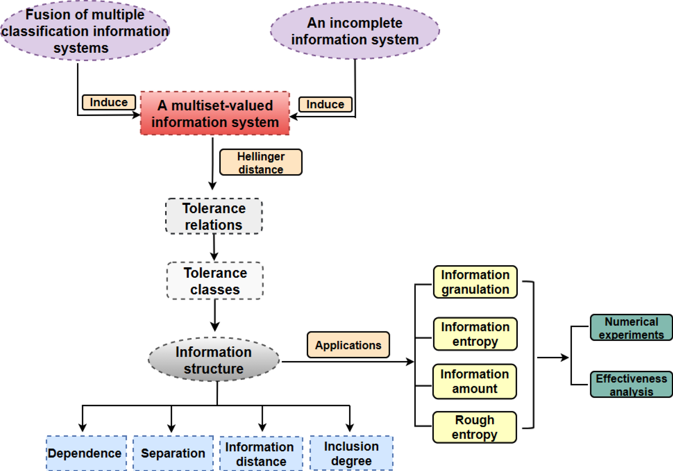
The research framework of this paper.

2 Preliminaries

In this paper, suppose that O is a non-empty finite set of objects, 2^O expresses the collection that is formed by all subsets of O and |X| indicates the cardinality of X ∈ 2^O. Put $O = {o_{1}, o_{2}, \dots, o_{n}} .$

2.1 Binary relations

For R ⊆ O × O, then R is a binary relation on O. If (o, o′) ∈ R, denoted by oRo′. A binary relation R is satisfied the following properties.

(1) reflexive, ∀ o ∈ O ⇒ oRo;

(2) symmetric, ∀ o, o′ ∈ O, oRo′ ⇒ o′Ro;

(3) transitive, ∀ o, o′, o″ ∈ O, oRo′ and o′Ro″ ⇒ oRo″.

Then, R is said to be an equivalence relation on O, if R is reflexive, symmetric and transitive; R is called a tolerance relation on O, if R is reflexive and symmetric.

2.2 Multisets

A multiset is a collection of elements in which an element may appear more than once. The number of occurrences of an element in a multiset is referred to as the multiplicity of this element. The cardinality of a multiset is the sum of the multiplicities of its elements [1].

Definition 2.1. [32] Suppose that X is a non-empty finite set. A multiset M drawn from X is characterized by a function $C_{M} : X \to ℕ$ , where $ℕ$ is the set of natural numbers.

For convenience, ∀ x ∈ U, C_M (x) is denoted by M (x) .

If M (x) = m, then it represents that x appears m times in M, we denote it by $m / x \in M or x \in^{m} M .$

For a non-empty finite set X = {x₁, x₂, …, x_s}, ∀ x_i ∈ X, M (x_i) = m_i, then M is denoted by {m₁/x₁, m₂/x₂, ⋯ , m_n/x_s}, i.e., $M = {m_{1} / x_{1}, m_{2} / x_{2}, \dots, m_{n} / x_{s}} .$

Definition 2.2.Given a non-empty finite set X. Let M₁ and M₂ be two multisets drawn from X. The equation, contain, union, intersection, addition and subtraction of M₁ and M₂ are defined as

(1) M₁ = M₂⇔ M₁ (x) = M₂ (x) (x ∈ X) ;

(2) M₁⊑ M₂ ⇔ M₁ (x) ≤ M₂ (x) (x ∈ X) ;

(3) P = M₁⊔ M₂ ⇔ P (x) = M₁ (x) ∨ M₂ (x) (x ∈ X) ;

(4) P = M₁ ⊓ M₂ ⇔ P (x) = M₁ (x) ∧ M₂ (x) (x ∈ X) .

(5) P = M₁⊕ M₂ ⇔ P (x) = M₁ (x) + M₂ (x) (x ∈ X) ;

(6) P = M₁ ⊖ M₂ ⇔ P (x) = (M₁ (x) - M₂ (x)) ∨0 (x ∈ X) .

2.3 Probability distribution sets

In the real world, there are many probabilistic data and related models proposed by Barbara et al. from the early 1990s [3, 4]. For example, patients who might have the flu are needed to be diagnosed by five doctors from some symptoms. Each patient has different degrees of symptoms that are headache={yes,no}, musclepain={yes,no} and temperature={normal,high,very high}. Five doctors will give the diagnosis results of patients’ symptoms based on their own experience, such as, for the symptoms of temperature, they diagnosed patient A as normal, normal, high, high and very high. These results can be denoted by a set, i.e., S = {normal, normal, high, high, very high}. Moreover, S = {normal, normal, high, high, very high} is expressed as a multiset S = {normal/2, high/2, very high/1}. In this multiset, the probability of occurrence of normal is 0.4, the probability of occurrence of high is 0.4, the probability of occurrence of very high is 0.2. In order to better express this phenomenon, a probability distribution set be defined as follows.

Definition 2.3. For a non-empty finite set X = {x₁, x₂, ⋯ , x_s}. Suppose $P = {\frac{x_{1}, x_{2}, \dots, x_{s}}{p_{1}, p_{2}, \dots, p_{s}}} .$ If for each i, 0 ≤ p_i ≤ 1 and $\sum_{i = 1}^{n} p_{i} = 1,$ then P is referred to as a probability distribution set(PDS) over X. If for any i, p_i is a rational number, P is referred to as a rational probability distribution set(RPDS); otherwise, P is referred to as an irrational probability distribution set(IRPDS).

From the above definition, P can be regarded as a map P : X → [0, 1] , namely, $\forall i, P (x_{i}) = p_{i} .$

Definition 2.4. For two non-empty finite sets X = {x₁, x₂, ⋯ , x_s} and Y = {y₁, y₂, ⋯ , y_t}. Suppose that P and Q are PDSs over X and Y, respectively. Denote $P = {\frac{x_{1}, x_{2}, \dots, x_{s}}{p_{1}, p_{2}, \dots, p_{s}}}, Q = {\frac{y_{1}, y_{2}, \dots, y_{t}}{q_{1}, q_{2}, \dots, q_{t}}} .$

(1) P and Q are said to be equal, if s = t, for each i, x_i = y_i and p_i = q_i. We write $P = Q;$

(2) P and Q are said to be approximately equal, if s = t and for each i, x_i = y_i. We write $P ≃ Q .$

clearly, P = Q ⇒ P ≃ Q.

Definition 2.5.Suppose that P and Q are two PDSs over X. Denote $P = {\frac{x_{1}, x_{2}, \dots, x_{s}}{p_{1}, p_{2}, \dots, p_{s}}}, Q = {\frac{x_{1}, x_{2}, \dots, x_{s}}{q_{1}, q_{2}, \dots, q_{s}}} .$ Then Hellinger distance between P and Q is defined by $HD (P, Q) = \frac{1}{\sqrt{2}} \sqrt{\sum_{i = 1}^{s} (\sqrt{p_{i}} - \sqrt{q_{i}})^{2}} .$ Apparently, $HD (P, Q) = \sqrt{1 - \sum_{i = 1}^{s} \sqrt{p_{i} q_{i}}} .$

2.4 Relationships between multisets and PDSs

In this subsection, we will prove that there exist relationships of one-to-one correspondence between multisets and PDSs. This result will be helpful for understanding why a multiset can been considered as a PDS.

Definition 2.6. For a non-empty finite set X = {x₁, x₂, ⋯ , x_s}. Suppose that M = {m₁/x₁, m₂/x₂, …, m_s/x_s} is a multiset drawn from X. Let $P_{M} = {\frac{x_{1}, x_{2}, \dots, x_{s}}{p_{1}, p_{2}, \dots, p_{s}}},$ where $p_{i} = \frac{m_{i}}{\sum_{i = 1}^{s} m_{i}}$ . Then P_M is called a RPDS over X induced by M.

Obviously, $\forall i, P_{M} (x_{i}) = p_{i} = \frac{m_{i}}{\sum_{i = 1}^{s} m_{i}} = \frac{M (x_{i})}{\sum_{i = 1}^{s} M (x_{i})} .$

Definition 2.7. For a non-empty finite set X = {x₁, x₂, ⋯ , x_s}. Suppose that $P = {\frac{x_{1}, x_{2}, \dots, x_{s}}{p_{1}, p_{2}, \dots, p_{s}}}$ is a RPDS over X. Denote (i) $\forall i, p_{i} = \frac{m_{i}}{n_{i}}$ , where m_i and n_i are two rational numbers; (ii) ∀i, n^* = k_in_i (k_i ∈ N), where n^* = [n₁, n₂, ⋯ , n_s] (the least common multiple of n₁, n₂,⋯, n_s); (iii) p₁ + p₂ + ⋯ + p_s = 1 ⇒ n^* = k₁m₁ + k₂m₂ + ⋯ + k_sm_s. Define $M_{P} = {k_{1} m_{1} / x_{1}, k_{2} m_{2} / x_{2}, \dots, k_{2} m_{2} / x_{s}} .$ Then M_P is a multiset drawn from X. We call M_P is the multiset induced by P.

Clearly, $\forall i, M_{P} (x_{i}) = k_{i} m_{i} = k_{i} p_{i} n_{i} = P (x_{i}) n^{*}$ = P (x_i) [n₁, n₂, ⋯ , n_s] .

Lemma 2.8.Given a non-empty set X = {x₁, x₂, ⋯ , x_s}. Suppose that M is a multiset drawn from X, P_M is the PDS induced by M and M_{P
_M} is the multiset induced by P_M. Then M_{P
_M} = M.

Proof. Denote $M (x_{1}) + M (x_{2}) + \dots + M (x_{s}) = ▵ .$

∀ i, $P_{M} (x_{i}) = p_{i} = \frac{m_{i}}{m_{1} + m_{2} + \dots + m_{s}}$ $= \frac{M (x_{i})}{M (x_{1}) + M (x_{2}) + \dots + M (x_{s})} ≐ \frac{m_{i}^{'}}{n_{i}^{'}} .$ Note that $“ n_{1}^{'} = n_{2}^{'} = \dots = n_{s}^{'} = ▵ "$ implies that $(n^{'})^{*} = [n_{1}^{'}, n_{2}^{'}, \dots, n_{s}^{'}] = ▵ .$

Then ∀ i, $M_{P_{M}} (x_{i}) = P_{M} (x_{i}) [n_{1}^{'}, n_{2}^{'}, \dots, n_{s}^{'}]$ $= \frac{M (x_{i})}{M (x_{1}) + M (x_{2}) + \dots + M (x_{s})} ▵ = M (x_{i}) .$ Thus, M_{P
_M} = M. □

Lemma 2.9.Given a non-empty set X = {x₁, x₂, ⋯ , x_s}. Suppose that P is a RPDS over X, M_P is the multiset induced by P and P_{M
_P} is the probability distribution set induced by M_P. Then P_{M
_P} = P.

Proof. For any i, denote $P (x_{i}) = p_{i} = \frac{m_{i}}{n_{i}}$ where m_i and n_i are two rational numbers. Denote $n^{*} = [n_{1}, n_{2}, \dots, n_{s}], \forall i, n^{*} = k_{i} n_{i} (k_{i} \in N) .$

Then ∀ i, $M_{P} (x_{i}) = k_{i} m_{i} = P (x_{i}) n^{*} .$

Note that ∀ i, $P_{M_{P}} (x_{i}) = \frac{M_{P} (x_{i})}{M_{P} (x_{1}) + M_{P} (x_{2}) + \dots + M_{P} (x_{s})} .$ Then ∀ i, $P_{M_{P}} (x_{i}) = \frac{P (x_{i}) n^{*}}{P (x_{1}) n^{*} + P (x_{2}) n^{*} + \dots + P (x_{s}) n^{*}}$ $= \frac{P (x_{i})}{P (x_{1}) + P (x_{2}) + \dots + P (x_{s})} = P (x_{i}) .$ Thus P_{M
_P} = P. □

Theorem 2.10.Given a non-empty set X = {x₁, x₂, ⋯ , x_s}. Denote $Ω = {M : M is a multiset drawn from X}$ and $Ψ = {P : P is a RPDS over X} .$ Then there exists a one-to-one correspondence between Ω and Ψ.

Proof. Suppose that f : Ω → Ψ and g : Ψ → Ω are two mappings, define $f (M) = P_{M}, \forall M \in Ω,$ $g (P) = M_{P}, \forall P \in Ψ .$

Then $\forall P \in Ψ, (f \circ g) (P) = f [g (P)] = f (M_{P}) = P_{M_{P}};$ $\forall M \in Ω, (g \circ f) (M) = g [f (M)] = g (P_{M}) = M_{P_{M}} .$

By Lemmas 2.8 and 2.9, we get $\forall P \in Ψ, (f \circ g) (P) = P;$ $\forall M \in Ω, (g \circ f) (M) = M .$

Thus f ∘ g = i_Ψ, g ∘ f = i_Ω, where i_Ψ is the identity mapping on Ψ, i_Ω is the identity mapping on Ω, respectively.

Hence, f and g are two one-to-one correspondences. This suggests that there exists a one-to-one correspondence between Ω and Ψ. □

Based on Theorem 2.10, a multiset is able to be considered as a RPDS. Below, we will deal with multisets like RPDSs.

3 Multiset-valued information systems

In this section, we introduce the concept of multiset-valued information system (MVIS), and define tolerance relations and rough approximations in a MVIS.

3.1 The concept of multiset-valued information system

In this subsection a MVIS can be regarded as the result of information fusion of multiple categorical ISs.

Definition 3.1. ([36]).Suppose that O is a set of objects and A is a set of attributes. Then the pair (O, A) is referred to as an information system (IS), if ∀ a ∈ A determines an information function a : U → V_a, where V_a = {a (o) : o ∈ O}.

Especially, if ∃ o ∈ O and a ∈ A such that a (o) is a missing value, denoted by a (o) =*, then (O, A) is called an incomplete information system (IIS).

Suppose that (O, A) is an IIS. For any a ∈ A, denote $V_{a}^{⋄} = V_{a} - {a (o) : a (o) = *} .$

Example 3.2Table 1 shows an IIS (O, A) about cars, where O = {o₁, o₂, ⋯ , o₉} and A = {a₁, a₂, a₃, a₄} express nine cars and four different performance metrics. Each car has varying degrees of performance, namely, price(a₁)={L = low, H = high}, size(a₂) ={C = compact, F = full}, engine(a₃)={D = diesel, G = gasoline}, max-speed(a₄)={L = low, M = medium, H = high}.

One can see from Table 1 that $V_{a_{1}}^{⋄} = V_{a_{1}} = {L, H}, V_{a_{2}}^{⋄} = {C, F}, V_{a_{3}}^{⋄} = {D, G}, V_{a_{4}}^{⋄} = {L, M, H} .$

Table 1
An IIS about cars

O a ₁ a ₂ a ₃ a ₄

o ₁ L C * L

o ₂ H F D H

o ₃ L F * H

o ₄ L C D M

o ₅ H * * M

o ₆ H C G *

o ₇ L F G L

o ₈ H * D H

o ₉ L C D L

O	a ₁	a ₂	a ₃	a ₄
o ₁	L	C	*	L
o ₂	H	F	D	H
o ₃	L	F	*	H
o ₄	L	C	D	M
o ₅	H	*	*	M
o ₆	H	C	G	*
o ₇	L	F	G	L
o ₈	H	*	D	H
o ₉	L	C	D	L

Definition 3.3. Suppose that (O, A) is an IS. Then the pair (O, A) is regarded as a multiset-valued information system (MVIS), if for each a ∈ A, a (o₁), a (o₂), ⋯ a (o_n) are multisets drawn from the same set.

If B ⊆ A, then (O, B) is known as a subsystem of (O, A).

Considering that internal structures of a MVIS are complex. For ease of understanding, we will reveal this internal structure in the following.

Let (O, A) be a MVIS, where O = {o₁, o₂, ⋯ , o_n} and A = {a₁, a₂, ⋯ , a_m} . For any i, a_i (o₁), a_i (o₂), ⋯ a_i (o_n) are multisets drawn from a same set. We denote the same set by X_i, namely, $X_{i} = {x_{i 1}, x_{i 2}, \dots, x_{{is}_{i}}} (i = 1, 2, \dots, m) .$ Then for each i, a_i (o₁), a_i (o₂), ⋯ a_i (o_n) can be expressed as the following multisets drawn from X_i: $a_{i} (o_{1}) = {k_{1}^{(1)} / x_{i 1}, k_{2}^{(1)} / x_{i 2}, \dots, k_{s_{i}}^{(1)} / x_{{is}_{i}}},$ $a_{i} (o_{2}) = {k_{1}^{(2)} / x_{i 1}, k_{2}^{(2)} / x_{i 2}, \dots, k_{s_{i}}^{(2)} / x_{{is}_{i}}},$ $\dots \dots \dots \dots \dots \dots \dots \dots \dots \dots \dots \dots \dots$ $a_{i} (o_{n}) = {k_{1}^{(n)} / x_{i 1}, k_{2}^{(n)} / x_{i 2}, \dots, k_{s_{i}}^{(n)} / x_{{is}_{i}}} .$

Definition 3.4.MSVIS Suppose that (O, A) is an IIS with O = {o₁, o₂, ⋯ , o_n}. Given a ∈ A. Denote $V_{a}^{⋄} = {a (o_{1}), a (o_{2}), \dots, a (o_{n})} - {*} ≜ {x_{1}, x_{2}, \dots, x_{s}} .$ Assuming that m_i expresses the number of occurrences of x_i in {x₁, x₂, ⋯ , x_s}, (i) if a (o) =*, then a (o) is replaced by {m₁/x₁, m₂/x₂, ⋯ , m_s/x_s}; (ii) if a (o) = x_j, then a (o) is replaced by ${0 / x_{1}, \dots, 0 / x_{j - 1}, 1 / x_{j - 1}, 0 / x_{j + 1}, \dots, 0 / x_{s}} .$ So it’s treated in this way, (O, A) can be called a MVIS induced by the IIS.

Next, we illustrate by an example that a MVIS can be induced by an IIS.

Example 3.5.(Continued from Example 3.2) The MVIS (O, A) is induced by an IIS in Table 2.

Table 2

An MVIS (O, A) is induced by an IIS.

O	a ₁	a ₂	a ₃	a ₄
o ₁	{0/H,1/L}	{1/C,0/F}	{4/D,2/G}	{1/L,0/M,0/H}
o ₂	{1/H,0/L}	{0/C,1/F}	{1/D,0/G}	{0/L,0/M,1/H}
o ₃	{0/H,1/L}	{0/C,1/F}	{4/D,2/G}	{0/L,0/M,1/H}
o ₄	{0/H,1/L}	{1/C,0/F}	{1/D,0/G}	{0/L,1/M,0/H}
o ₅	{1/H,0/L}	{4/C,3/F}	{4/D,2/G}	{0/L,1/M,0/H}
o ₆	{1/H,0/L}	{1/C,0/F}	{0/D,1/G}	{3/L,2/M,3/H}
o ₇	{0/H,1/L}	{0/C,1/F}	{0/D,1/G}	{1/L,0/M,0/H}
o ₈	{1/H,0/L}	{4/C,3/F}	{1/D,0/G}	{0/L,0/M,1/H}
o ₉	{0/H,1/L}	{1/C,0/F}	{1/D,0/G}	{1/L,0/M,0/H}

The following example illustrates the background of a MVIS. In practical application of evaluating the credit card applicant’s credit rating, a credit card applicant is evaluated by multiple experts, and may have dissimilar evaluation results.

Example 3.6. Assume that each credit card applicant is evaluated by five experts, and each expert’s evaluation results of credit card applicants corresponded to an information table (see Tables 3-7). Then the five information tables can be synthesized into a MVIS (see Table 8). In Table 3, O = {o₁, o₂, ⋯ , o₆} and A = {a₁, a₂, a₃, a₄} present six credit card applicants and four different evaluation characteristics, respectively, namely, education(a₁)={G = good, A = average, P = poor}, salary(a₂)={H = high, M = medium, L = low}, age(a₃)={O = old, Y = young}, consumption(a₄)= {H = high, M = medium, L = low}.

Put X₁ = {G, A, P}, X₂ = {H, M, L}, X₃ = {O, Y} and X₄ = {H, M, L}. Then ∀ o ∈ O, a₁ (o), a₂ (o), a₃ (o)and a₄ (o) are four multisets drawn from X₁, X₂, X₃ and X₄, respectively.

As can be seen from this example, a MVIS (see Table 8) may be the result of information fusion of multi-classified ISs or multi-source IS (see Tables 3-7).

Table 3

expert-1

O	a ₁	a ₂	a ₃	a ₄
o ₁	A	M	O	H
o ₂	G	H	O	M
o ₃	A	H	Y	M
o ₄	P	L	Y	L
o ₅	G	M	Y	H
o ₆	A	L	O	M

Table 4

expert-2

O	a ₁	a ₂	a ₃	a ₄
o ₁	G	H	O	H
o ₂	P	M	Y	M
o ₃	A	H	Y	M
o ₄	P	L	O	L
o ₅	G	H	Y	H
o ₆	A	L	O	H

Table 5

expert-3

O	a ₁	a ₂	a ₃	a ₄
o ₁	A	H	Y	M
o ₂	P	H	O	H
o ₃	A	M	Y	M
o ₄	G	H	O	L
o ₅	G	H	O	M
o ₆	P	L	Y	H

Table 6

expert-4

O	a ₁	a ₂	a ₃	a ₄
o ₁	P	H	Y	M
o ₂	G	H	Y	H
o ₃	A	M	O	H
o ₄	G	L	Y	L
o ₅	G	M	Y	M
o ₆	A	L	O	H

Table 7

expert-1

O	a ₁	a ₂	a ₃	a ₄
o ₁	G	H	O	H
o ₂	G	M	Y	H
o ₃	P	M	O	M
o ₄	P	L	Y	L
o ₅	G	H	O	M
o ₆	A	L	O	H

Table 8

A MVIS is composed of Tables 3-7

O	a ₁	a ₂	a ₃	a ₄
o ₁	{2/G,2/A,1/P}	{4/H,1/M,0/L}	{2/Y,3/O}	{3/H,2/M,0/L}
o ₂	{3/G,0/A,2/P}	{3/H,2/M,0/L}	{3/Y,2/O}	{3/H,2/M,0/L}
o ₃	{0/G,4/A,1/P}	{2/H,3/M,0/L}	{3/Y,2/O}	{1/H,4/M,0/L}
o ₄	{2/G,0/A,3/P}	{1/H,0/M,4/L}	{3/Y,2/O}	{0/H,0/M,5/L}
o ₅	{5/G,0/A,0/P}	{3/H,2/M,0/L}	{3/Y,2/O}	{2/H,3/M,0/L}
o ₆	{0/G,4/A,1/P}	{0/H,0/M,5/L}	{1/Y,4/O}	{4/H,1/M,0/L}

3.2 Tolerance relations and rough approximations in a MVIS

In this subsection, we provide the tolerance relation in each subsystem of a MVIS based on Hellinger distance.

Definition 3.7.Let (O, A) be a MVIS. Given B ⊆ A and θ ∈ [0, 1]. Define $T_{B}^{θ} = {(o, o^{'}) \in O \times O : \forall a \in B, HD (P_{a (o)}, P_{a (o^{'})}) \leq θ},$ where P_a(o) and P_a(o′) are the PDSs induced by a (o) and a (o′), respectively.

Clearly, $T_{B}^{θ}$ is a tolerance relation on O and $T_{B}^{θ} = ⋂_{a \in B} T_{a}^{θ}$ where $T_{a}^{θ} = T_{{a}}^{θ}$ .

Let $T_{B_{1}}^{θ}$ and $T_{B_{2}}^{θ}$ be two tolerance relations of attribute subset B₁ and B₂ with respect to θ, respectively, we say that $T_{B_{1}}^{θ}$ is finer than $T_{B_{2}}^{θ}$ if $T_{B_{1}}^{θ} \subseteq T_{B_{2}}^{θ}$ . According to the Definition 3.7, we know that objects "o" and "o’" are indistinguishable if for each a ∈ B, HD (P_a(o), P_a(o′)) ≤ θ; otherwise, they are distinguishable; the finer a tolerance relation, the greater its distinguishing ability. There are two factors that influence a tolerance relation. One is the parameter θ, the other is the attribute subset B. For a given attribute subset B, the tolerance relation becomes finer as the the parameter θ smaller; For a given parameter θ, the tolerance relation becomes finer as the attribute subset B bigger.

Definition 3.8.Let (O, A) be a MVIS. Given θ ∈ [0, 1] and B ⊆ A. Then the θ-tolerance class of o ∈ O under $T_{B}^{θ}$ is defined as $T_{B}^{θ} (o) = {o^{'} \in O : (o, o^{'}) \in T_{B}^{θ}} .$

Clearly, $T_{B}^{θ} (o) = ⋂_{a \in B} T_{a}^{θ} (o) .$

Theorem 3.9.Suppose that (O, A) is a MVIS and B₁, B₂, B ⊆ C. Given θ₁, θ₂ ∈ [0, 1], then the following properties are hold:

(1) If B₁ ⊆ B₂, ∀ o ∈ O, then $T_{B_{2}}^{θ} (o) \subseteq T_{B_{1}}^{θ} (o);$

(2) If 0 ≤ θ₁ < θ₂ ≤ 1, then $T_{B}^{θ_{1}} (o) \subseteq T_{B}^{θ_{2}} (o) .$

Proof. Obviously. □

Definition 3.10.Let (O, A) be a MVIS. Given X ∈ 2^O, B ⊆ A and θ ∈ [0, 1]. Based on the approximation space $(O, T_{B}^{θ})$ , a pair of operations $\underline{T_{B}^{θ}}$ , $\bar{T_{B}^{θ}}$ : 2^O ⟶ 2^O are defined by $\underline{T_{B}^{θ}} (X) = {o \in O : T_{B}^{θ} (o) \subseteq X},$ $\bar{T_{B}^{θ}} (X) = {o \in O : T_{B}^{θ} (o) \cap X \neq \emptyset} .$ Then $\underline{T_{B}^{θ}} (X)$ and $\bar{T_{B}^{θ}} (X)$ are called θ-lower and θ-upper approximations of X, respectively.

Theorem 3.11.Let (O, A) be a MVIS. Given X, Y ∈ 2^O, B ⊆ A and θ ∈ [0, 1]. Then the following properties hold. (1) $\bar{T_{B}^{θ}} (\emptyset) = \underline{T_{B}^{θ}} (\emptyset) = \emptyset$ , $\underline{T_{B}^{θ}} (O) = \bar{T_{B}^{θ}} (O) = O$ ; (2) $\underline{T_{B}^{θ}} (X) \subseteq X \subseteq \bar{T_{B}^{θ}} (X)$ ; (3) $X \subseteq Y \Rightarrow \underline{T_{B}^{θ}} (X) \subseteq \underline{T_{B}^{θ}} (Y),$ $\bar{T_{B}^{θ}} (X) \subseteq \bar{T_{B}^{θ}} (Y)$ ; (4) If B₁ ⊆ B₂ ⊆ A, then $\underline{T_{B_{1}}^{θ}} (X) \subseteq \underline{T_{B_{2}}^{θ}} (X), \bar{T_{B_{2}}^{θ}} (X) \subseteq \bar{T_{B_{1}}^{θ}} (X);$ (5) If 0 < θ₁ ≤ θ₂ ≤ 1, then $\underline{T_{B}^{θ_{2}}} (X) \subseteq \underline{T_{B}^{θ_{1}}} (X), \bar{T_{B}^{θ_{1}}} (X) \subseteq \bar{T_{B}^{θ_{2}}} (X);$ (6) $\underline{T_{B}^{θ}} (X \cap Y) = \underline{T_{B}^{θ}} (X) \cap \underline{T_{B}^{θ}} (Y)$ , $\bar{T_{B}^{θ}} (X \cap Y) = \bar{T_{B}^{θ}} (X) \cup \bar{T_{B}^{θ}} (Y)$ ;(7) $\underline{T_{B}^{θ}} (O - X) = O - \bar{T_{B}^{θ}} (X)$ , $\bar{T_{B}^{θ}} (O - X) = O - \underline{T_{B}^{θ}} (X)$ .

Proof. Obviously. □

4 Information structures in a MVIS

In this section, we study information structures in a MVIS.

4.1 The concept of information structures in a MVIS

From the perspective of GrC, information structures refer to a mathematical structure of the family of information granules granulated from a data set. Considering that a set vector is better than family of sets in displaying the internal structure of an information structure, a mathematical structure of the family of information granules is showed by a set vector.

Definition 4.1. Let (O, A) be a MVIS. Given θ ∈ [0, 1]. Then for B ⊆ A, the information structure of the subsystem (O, B) is defined as $S^{θ} (B) = (T_{B}^{θ} (o_{1}), T_{B}^{θ} (o_{2}), \dots, T_{B}^{θ} (o_{n})) .$

Especially, if ∀ i, $T_{B}^{θ} (o_{i}) = U$ , we denote S^θ (U) = (U, U, ⋯ , U) ; if ∀ i, $T_{B}^{θ} (o_{i}) = {o_{i}}$ , we denote S^θ (π) = ({o₁} , {o₂} , ⋯ , {o_n}) .

Definition 4.2. Let (O, A) be a MVIS. Denote $S (O, C (A)) ≜ S (O)$ is called the information structure base of (O, C (A)), where C (A) is the collection of all subsets of attribute A.

Definition 4.3. Let (O, A) be a MVIS. Given θ₁, θ₂ ∈ [0, 1] and B₁, B₂ ⊆ A. Suppose that S^{θ
₁} (B₁), S^{θ
₂} (B₂) are the information structures of the subsystems (O, B₁) and (O, B₂), respectively. Then S^{θ
₁} (B₁) and S^{θ
₂} (B₂) are called to the same, if ∀ o ∈ O, $T_{B_{1}}^{θ_{1}} (o) = T_{B_{2}}^{θ_{2}} (o)$ , we write as S^{θ
₁} (B₁) ≈ S^{θ
₂} (B₂).

Definition 4.4. Let (O, A) be a MVIS. Given θ₁, θ₂ ∈ [0, 1] and B₁, B₂ ⊆ A. Suppose that S^{θ
₁} (B₁), S^{θ
₂} (B₂) are the information structures of the subsystems (O, B₁) and (O, B₂), respectively.

(1) S^{θ
₁} (B₁) is said to be dependent on S^{θ
₂} (B₂), if ∀ o ∈ O, $T_{B_{1}}^{θ_{1}} (o) \subseteq T_{B_{2}}^{θ_{2}} (o)$ , we denote by S^{θ
₁} (B₁) ⪯ S^{θ
₂} (B₂); S^{θ
₁} (B₁) is said to be dependent strictly on S^{θ
₂} (B₂), if S^{θ
₁} (B₁) ⪯ S^{θ
₂} (B₂) and S^{θ
₁} (B₁) notapproxS^{θ
₂} (B₂), we write as S^{θ
₁} (B₁) ≺ S^{θ
₂} (B₂);

(2) S^{θ
₁} (B₁) is said to be dependent partially on S^{θ
₂} (B₂), if ∃ o ∈ O, $T_{B_{1}}^{θ_{1}} (o) \subseteq T_{B_{2}}^{θ_{2}} (o)$ , we denote by S^{θ
₁} (B₁) ⊑ S^{θ
₂} (B₂); S^{θ
₁} (B₁) is said to be dependent partially strictly on S^{θ
₂} (B₂), if S^{θ
₁} (B₁) ⊑ S^{θ
₂} (B₂) and S^{θ
₁} (B₁) notapproxS^{θ
₂} (B₂), we write as S^{θ
₁} (B₁) ⊏ S^{θ
₂} (B₂);

(3) S^{θ
₁} (B₁) is said to be independent on S^{θ
₂} (B₂), if ∀ o ∈ O, $T_{B_{1}}^{θ_{1}} (o) ⊈ T_{B_{2}}^{θ_{2}} (o)$ , we denote by S^{θ
₁} (B₁) ⋈ S^{θ
₂} (B₂).

Example 4.5.(Continued from Example 3.5) Pick θ₁ = 0.3 and θ₂ = 0.4. Given B₁ = {a₂}, B₂ = {a₃} and B₃ = {a₂, a₄}. By Definition 4.1, we can compute

S^{θ
₁} (B₁) = ({x₁, x₄, x₆, x₉} , {x₂, x₃, x₇} , {x₂, x₃, x₇} , {x₁, x₄, x₆, x₉} , {x₅, x₈} , {x₁, x₄, x₆, x₉} , {x₂, x₃, x₇} , {x₅, x₈} , {x₁, x₄, x₆, x₉}) ;∥S^{θ
₂} (B₂) = ({x₁, x₃, x₅} , {x₂, x₄, x₈, x₉} , {x₁, x₃, x₅} , {x₂, x₄, x₈, x₉} , {x₁, x₃, x₅} , {x₆, x₇} , {x₆, x₇} , {x₂, x₄, x₈, x₉} , {x₂, x₄, x₈, x₉}) ;∥S^{θ
₂} (B₃) = ({x₁, x₉} , {x₂, x₃} , {x₂, x₃} , {x₄} , {x₅} , {x₆} , {x₇} , {x₈} , {x₁, x₉}) .

Thus, $S^{θ_{2}} (B_{3}) ≺ S^{θ_{1}} (B_{1}), S^{θ_{1}} (B_{1}) ⋈ S^{θ_{2}} (B_{2}) .$

4.2 Relationships between information structures in a MVIS

In this subsection, we study relationships between information structures in a MVIS from two aspects of dependence and separation.

4.2.1 Dependence between information structures in a MVIS

Definition 4.6.Let (O, A) be a MVIS. Given θ₁, θ₂, θ₃ ∈ [0, 1] and B₁, B₂, B₃ ⊆ A. Suppose that S^{θ
₁} (B₁), S^{θ
₂} (B₂), S^{θ
₂} (B₃) are the information structures of the subsystems (O, B₁), (O, B₂), (O, B₃), respectively. Then a mapping D : S (O) × S (O) → [0, 1] is called the inclusion degree on S (O), if(1) 0 ≤ D (S^{θ
₂} (B₂)/S^{θ
₁} (B₁)) ≤1;

(2) S^{θ
₁} (B₁) ⪯ S^{θ
₂} (B₂) implies $D (S^{θ_{2}} (B_{2}) / S^{θ_{1}} (B_{1})) = 1;$ (3) S^{θ
₁} (B₁) ⊑ S^{θ
₂} (B₂) ⊑ S^{θ
₃} (B₃) implies $D (S^{θ_{1}} (B_{1}) / S^{θ_{3}} (B_{3})) \leq D (S^{θ_{1}} (B_{1}) / S^{θ_{2}} (B_{2})) .$

Definition 4.7.Let (O, A) be a MVIS. Given θ₁, θ₂ ∈ [0, 1] and B₁, B₂ ⊆ A. DefineD (S^{θ
₁} (B₁)/S^{θ
₂} (B₂)) $= \sum_{i = 1}^{n} \frac{| T_{B_{2}}^{θ_{2}} (o_{i}) |}{\sum_{i = 1}^{n} | T_{B_{2}}^{θ_{2}} (o_{i}) |} χ_{T_{B_{2}}^{θ_{2}} (o_{i})} (T_{B_{1}}^{θ_{1}} (o_{i})),$ where $χ_{T_{B_{2}}^{θ_{2}} (o_{i})} (T_{B_{1}}^{θ_{1}} (o_{i})) = {\begin{matrix} 1, & if T_{B_{1}}^{θ_{1}} (o_{i}) \subseteq T_{B_{2}}^{θ_{2}} (o_{i}), \\ 0, & if T_{B_{1}}^{θ_{1}} (o_{i}) ⊈ T_{B_{2}}^{θ_{2}} (o_{i}) . \end{matrix}$

Proposition 4.8. D in Definition 4.7 is the inclusion degree under Definition 4.6.

Proof. Obviously. □

The following theorem shows that the relationship between information structures can be quantitatively described by inclusion degree in a MVIS.

Theorem 4.9. Let (O, A) be a MVIS. Given θ₁, θ₂ ∈ [0, 1] and B₁, B₂ ⊆ A. Then $(1) S^{θ_{1}} (B_{1}) ⪯ S^{θ_{2}} (B_{2}) \Leftrightarrow D (S^{θ_{2}} (B_{2}) / S^{θ_{1}} (B_{1})) = 1;$ $(2) S^{θ_{1}} (B_{1}) ⋈ S^{θ_{2}} (B_{2}) \Leftrightarrow D (S^{θ_{2}} (B_{2}) / S^{θ_{1}} (B_{1})) = 0;$ $(3) S^{θ_{1}} (B_{1}) ⊑ S^{θ_{2}} (B_{2}) \Leftrightarrow 0 < D (S^{θ_{2}} (B_{2}) / S^{θ_{1}} (B_{1})) \leq 1 .$

Proof. (1) “⇒" is obvious.

“⇐". Denote $| T_{B_{2}}^{θ_{2}} (o_{i}) | = q_{i},$ $q = \sum_{i = 1}^{n} q_{i}$ . Since D (S^{θ
₂} (B₂)/S^{θ
₁} (B₁)) =1, by Definition 4.7 we can obtain $\sum_{i = 1}^{n} \frac{q_{i}}{q} χ_{T_{B_{2}}^{θ_{2}} (o_{i})} (T_{B_{1}}^{θ_{1}} (o_{i})) = 1 .$ Thus, for any i, $χ_{T_{B_{2}}^{θ_{2}} (o_{i})} (T_{B_{1}}^{θ_{1}} (o_{i})) = 1 .$ It follows that for each i, $T_{B_{1}}^{θ_{1}} (o_{i}) \subseteq T_{B_{2}}^{θ_{2}} (o_{i})$ . Hence S^{θ
₁} (B₁) ⪯ S^{θ
₂} (B₂).(2) “⇒". Since S^{θ
₁} (B₁) ⋈ S^{θ
₂} (B₂), for any i, $T_{B_{1}}^{θ_{1}} (o_{i}) ⊈ T_{B_{2}}^{θ_{2}} (o_{i})$ . Thus, for each i, $χ_{T_{B_{2}}^{θ_{2}} (o_{i})} (T_{B_{1}}^{θ_{1}} (o_{i})) = 0 .$ Thus, D (S^{θ
₂} (B₂)/S^{θ
₁} (B₁)) =0.“⇐". Since D (S^{θ
₂} (B₂)/S^{θ
₁} (B₁)) =0, then for each i, $χ_{T_{B_{2}}^{θ_{2}} (o_{i})} (T_{B_{1}}^{θ_{1}} (o_{i})) = 0 .$ we can obtain ∀ i, $T_{B_{1}}^{θ_{1}} (o_{i}) ⊈ T_{B_{2}}^{θ_{2}} (o_{i})$ . Thus, S^{θ
₁} (B₁) ⋈ S^{θ
₂} (B₂).(3) This holds by (1) and (2). □

4.2.2 Information distance between information structures in a MVIS

In non-deterministic reasoning, the distance between uncertain structures plays an important role in reasoning. Taking into consideration of separation between information structures of a MVIS, we put forward the notion of information distance to differentiate two given information structures in the same MVIS and research some of its properties.

For X, Y ∈ 2^O, denote $X \oplus Y = X \cup Y - X \cap Y .$ Then X ⊕ Y is referred to as the symmetric difference X and Y.

Apparently, ∣X⊕ Y ∣ = ∣ X ∪ Y ∣ - ∣ X ∩ Y ∣.

Lemma 4.10.Let X, Y, Z ⊆ O. Then $∣ X \oplus Y ∣ + ∣ Y \oplus Z ∣ \geq ∣ X \oplus Z ∣ .$

Proof. Clearly. □

Lemma 4.11. Let X, Y, Z ⊆ O. If X ⊆ Y ⊆ Z or Z ⊆ Y ⊆ X, then $∣ X \oplus Y ∣ + ∣ Y \oplus Z ∣ = ∣ X \oplus Z ∣ .$

Proof. Obviously. □

Definition 4.12. ([17]). For a nonempty set M. Suppose that $ρ : M \times M \to ℝ$ is a mapping. If ρ meets the following conditions:

(1) (Nonnegativity) ∀ m, m′ ∈ M, ρ (m, m′) ≥0 and ρ (m, m) =0;

(2) (Symmetry) ∀ m, m′ ∈ M, ρ (m, m′) = ρ (m′, m);

(3) (Trigonometric inequality) ∀ m, m′, m″ ∈ M, ρ (m, m″) ≤ ρ (m, m′) + ρ (m′, m″).

Under these circumstances, ρ is called a pseudo-metric on M.

Definition 4.13.Let (O, A) be a MVIS. Given θ₁, θ₂ ∈ [0, 1] and B₁, B₂ ⊆ A. Suppose that S^{θ
₁} (B₁), S^{θ
₂} (B₂) are the information structures of the subsystems (O, B₁) and (O, B₂), respectively. Information distance between S^{θ
₁} (B₁) and S^{θ
₂} (B₂) is defined by $ρ (S^{θ_{1}} (B_{1}), S^{θ_{2}} (B_{2})) = \frac{1}{n^{2}} \sum_{i = 1}^{n} ∣ T_{B_{1}}^{θ_{1}} (o_{i}) \oplus T_{B_{2}}^{θ_{2}} (o_{i}) ∣ .$

Theorem 4.14. Let (O, A) be a MVIS. Then (S (O, C (A)) , ρ) is a pseudo-metric space.

Proof. Suppose B₁, B₂, B₃ ⊆ A. Given θ₁, θ₂, θ₃ ∈ [0, 1]. Obviously,ρ (S^{θ
₁} (B₁) , S^{θ
₁} (B₁)) =0, ρ (S^{θ
₁} (B₁) , S^{θ
₂} (B₂)) ≥0, ρ (S^{θ
₁} (B₁) , S^{θ
₂} (B₂)) = ρ (S^{θ
₂} (B₂) , S^{θ
₁} (B₁)). By Lemma 4.10, for any i, $∣ T_{B_{1}}^{θ_{1}} (o_{i}) \oplus T_{B_{2}}^{θ_{2}} (o_{i}) ∣ + ∣ T_{B_{2}}^{θ_{2}} (o_{i}) \oplus T_{B_{3}}^{θ_{3}} (o_{i}) ∣ \geq ∣ T_{B_{1}}^{θ_{1}} (o_{i}) \oplus T_{B_{3}}^{θ_{3}} (o_{i}) ∣$ . Then, ρ (S^{θ
₁} (B₁) , S^{θ
₂} (B₂)) + ρ (S^{θ
₂} (B₂) , S^{θ
₃} (B₃))

$= \frac{1}{n^{2}} \sum_{i = 1}^{n} ∣ T_{B_{1}}^{θ_{1}} (o_{i}) \oplus T_{B_{2}}^{θ_{2}} (o_{i}) ∣ + \frac{1}{n^{2}} \sum_{i = 1}^{n} ∣ T_{B_{2}}^{θ_{2}} (o_{i}) \oplus T_{B_{3}}^{θ_{3}} (o_{i}) ∣$

$= \frac{1}{n^{2}} \sum_{i = 1}^{n} (∣ T_{B_{1}}^{θ_{1}} (o_{i}) \oplus T_{B_{2}}^{θ_{2}} (o_{i}) ∣ + ∣ T_{B_{2}}^{θ_{2}} (o_{i}) \oplus T_{B_{3}}^{θ_{3}} (o_{i}) ∣)$

$\geq \frac{1}{n^{2}} \sum_{i = 1}^{n} ∣ T_{B_{1}}^{θ_{1}} (o_{i}) \oplus T_{B_{3}}^{θ_{3}} (o_{i}) ∣$ = ρ (S^{θ
₁} (B₁) , S^{θ
₃} (B₃)) Thus, (S (O, C (A)) , ρ) is a pseudo-metric space. □

Proposition 4.15. Let (O, A) be a MVIS. Given θ₁, θ₂, θ_π, θ_U ∈ [0, 1] and B₁, B₂ ⊆ A. (1) $0 \leq ρ (S^{θ_{1}} (B_{1}), S^{θ_{2}} (B_{2})) \leq 1 - \frac{1}{n}$ . (2) If S^{θ
₁} (B₁) ⪯ S^{θ
₂} (B₂), then $ρ (S^{θ_{1}} (B_{1}), S^{θ_{π}} (π)) \leq ρ (S^{θ_{2}} (B_{2}), S^{θ_{π}} (π));$ (3) If S^{θ
₁} (B₁) ⪯ S^{θ
₂} (B₂), thenρ (S^{θ
₁} (B₁) , S^{θ
_U} (U)) ≥ ρ (S^{θ
₂} (B₂) , S^{θ
_U} (U)).

Proof. (1) For any i, $∣ T_{B_{1}}^{θ_{1}} (o_{i}) \cup T_{B_{2}}^{θ_{2}} (o_{i}) ∣ \leq n,$ $1 \leq ∣ T_{B_{1}}^{θ_{1}} (o_{i}) \cap T_{B_{2}}^{θ_{2}} (o_{i}) ∣ (i = 1, 2, \dots, n) .$

Then, $0 \leq ∣ T_{B_{1}}^{θ_{1}} (o_{i}) \oplus T_{B_{2}}^{θ_{2}} (o_{i}) ∣ \leq n - 1 (i = 1, 2, \dots, n) .$ Thus, $0 \leq ρ (S^{θ_{1}} (B_{1}), S^{θ_{2}} (B_{2})) \leq \frac{1}{n^{2}} \sum_{i = 1}^{n} (n - 1) = 1 - \frac{1}{n} .$

(2) Since S^{θ
₁} (B₁) ⪯ S^{θ
₂} (B₂), ∀ i, $T_{B_{1}}^{θ_{1}} (o_{i}) \subseteq T_{B_{2}}^{θ_{2}} (o_{i})$ . Thus, ∀ i, $∣ T_{B_{1}}^{θ_{1}} (o_{i}) ∣ \leq ∣ T_{B_{2}}^{θ_{2}} (o_{i}) ∣$ . By definition 4.13,

$ρ (S^{θ_{1}} (B_{1}), S^{θ_{π}} (π)) = \frac{1}{n^{2}} \sum_{i = 1}^{n} ∣ T_{B_{1}}^{θ_{1}} (o_{i}) \oplus {o_{i}} ∣ = \frac{1}{n^{2}} \sum_{i = 1}^{n} (∣ T_{B_{1}}^{θ_{1}} (o_{i}) \cup {o_{i}} ∣ - ∣ T_{B_{1}}^{θ_{1}} (o_{i}) \cap {o_{i}} ∣)$ $= \frac{1}{n^{2}} \sum_{i = 1}^{n} (∣ T_{B_{1}}^{θ_{1}} (o_{i}) ∣ - 1) \leq \frac{1}{n^{2}} \sum_{i = 1}^{n} (∣ T_{B_{2}}^{θ_{2}} (o_{i}) ∣ - 1) = ρ (S^{θ_{2}} (B_{2}), S^{θ_{π}} (π)) .$ (3) Note that S^{θ
₁} (B₁) ⪯ S^{θ
₂} (B₂), ∀ i, $T_{B_{1}}^{θ_{1}} (o_{i}) \subseteq T_{B_{2}}^{θ_{2}} (o_{i}) .$ Thus, $ρ (S^{θ_{1}} (B_{1}), S^{θ_{U}} (U)) = \frac{1}{n^{2}} \sum_{i = 1}^{n} ∣ T_{B_{1}}^{θ_{1}} (o_{i}) \oplus U ∣ = \frac{1}{n^{2}} \sum_{i = 1}^{n} (∣ T_{B_{1}}^{θ_{1}} (o_{i}) \cup U ∣ - ∣ T_{B_{1}}^{θ_{1}} (o_{i}) \cap U ∣)$ $= \frac{1}{n^{2}} \sum_{i = 1}^{n} (n - ∣ T_{B_{1}}^{θ_{1}} (o_{i}) ∣) \geq \frac{1}{n^{2}} \sum_{i = 1}^{n} (n - ∣ T_{B_{2}}^{θ_{2}} (o_{i}) ∣) = ρ (S^{θ_{2}} (B_{2}), S^{θ_{U}} (U)) .$ □

Proposition 4.16. Let (O, A) be a MVIS. Given θ, θ_π, θ_U ∈ [0, 1] and B ⊆ A, $ρ (S^{θ} (B), S^{θ_{π}} (π)) + ρ (S^{θ} (B), S^{θ_{U}} (U)) = 1 - \frac{1}{n} .$

Proof. By Definition 4.13,

ρ (S^θ (B) , S^{θ
_π} (π)) + ρ (S^θ (B) , S^{θ
_U} (U)) $= \frac{1}{n^{2}} \sum_{i = 1}^{n} ∣ T_{B}^{θ} (o_{i}) \oplus {o_{i}} ∣ + \frac{1}{n^{2}} \sum_{i = 1}^{n} ∣ T_{B}^{θ} (o_{i}) \oplus U ∣$ $= \frac{1}{n^{2}} \sum_{i = 1}^{n} (∣ T_{B}^{θ} (o_{i}) ∣ - 1) + \frac{1}{n^{2}} \sum_{i = 1}^{n} (n - ∣ T_{B}^{θ} (o_{i}) ∣)$

$= \frac{1}{n^{2}} \sum_{i = 1}^{n} (n - 1) = 1 - \frac{1}{n}$ . □

Proposition 4.17. Let (O, A) be a MVIS. Given θ₁, θ₂, θ₃ ∈ [0, 1] and B₁, B₂, B₃ ⊆ A. Suppose S^θ
₁ (B₁) ⪯ S^θ
₂ (B₂) ⪯ S^θ
₃ (B₃) or S^θ
₃ (B₃) ⪯ S^θ
₂ (B₂) ⪯ S^θ
₁ (B₁), thenρ (S^θ
₁ (B₁) , S^θ
₂ (B₂)) + ρ (S^θ
₂ (B₂) , S^θ
₃ (B₃))= ρ (S^θ
₁ (B₁) , S^θ
₃ (B₃)) .

Proof. By Definition 4.4, S^{θ
₁} (B₁) ⪯ S^{θ
₂} (B₂) ⪯ S^{θ
₃} (B₃) or S^{θ
₃} (B₃) ⪯ S^{θ
₂} (B₂) ⪯ S^{θ
₁} (B₁).Then, $T_{B_{1}}^{θ_{1}} (o_{i}) \subseteq T_{B_{2}}^{θ_{2}} (o_{i}) \subseteq T_{B_{3}}^{θ} (o_{i})$ or $T_{B_{3}}^{θ} (o_{i}) \subseteq T_{B_{2}}^{θ_{2}} (o_{i}) \subseteq T_{B_{1}}^{θ_{1}} (o_{i}) (i = 1, 2, \dots, n) .$ By Lemma 4.11, $∣ T_{B_{1}}^{θ_{1}} (o_{i}) \oplus T_{B_{2}}^{θ_{2}} (o_{i}) ∣ + ∣ T_{B_{2}}^{θ_{2}} (o_{i}) \oplus T_{B_{3}}^{θ_{3}} (o_{i}) ∣$ $= ∣ T_{B_{1}}^{θ_{1}} (o_{i}) \oplus T_{B_{3}}^{θ_{3}} (o_{i}) ∣ (i = 1, 2, \dots, n) .$ Thus, ρ (S^{θ
₁} (B₁) S^{θ
₂} (B₂)) + ρ (S^{θ
₂} (B₂) , S^{θ
₃} (B₃)) $= \frac{1}{n^{2}} \sum_{i = 1}^{n} ∣ T_{B_{1}}^{θ_{1}} (o_{i}) \oplus T_{B_{2}}^{θ_{2}} (o_{i}) ∣ + \frac{1}{n^{2}} \sum_{i = 1}^{n} ∣ T_{B_{2}}^{θ_{2}} (o_{i}) \oplus T_{B_{3}}^{θ_{3}} (o_{i}) ∣ = \frac{1}{n^{2}} \sum_{i = 1}^{n} (∣ T_{B_{1}}^{θ_{1}} (o_{i}) \oplus T_{B_{2}}^{θ_{2}} (o_{i}) ∣ + ∣ T_{B_{2}}^{θ_{2}} (o_{i}) \oplus T_{B_{3}}^{θ_{3}} (o_{i}) ∣) = \frac{1}{n^{2}} \sum_{i = 1}^{n} ∣ T_{B_{1}}^{θ_{1}} (o_{i}) \oplus T_{B_{3}}^{θ_{3}} (o_{i}) ∣ = ρ (S^{θ_{1}} (B_{1}), S^{θ_{3}} (B_{3}))$ . □

To illustrate the rationality of the above results, an example is given below.

Example 4.18. (Continued from Example 4.5) Pick θ_U = 1 . Given B₄ = {a₂, a₃, a₄} . ComputeS^{θ
₂} (B₄) =

({x₁} , {x₂} , {x₃} , {x₄} , {x₅} , {x₆} , {x₇} , {x₈} , {x₉}) , S^{θ
_U} (B₄) = (U, U, ⋯ , U) .Denote $S^{θ_{2}} (B_{4}) ≜ S^{θ_{π}} (π), S^{θ_{U}} (B_{3}) ≜ S^{θ_{U}} (U) .$

This example illustrates the following facts:(1) By Definition 4.13, calculate $ρ (S^{θ_{2}} (B_{3}), S^{θ_{U}} (U)) = \frac{68}{81},$ $ρ (S^{θ_{1}} (B_{1}), S^{θ_{U}} (U)) = \frac{52}{81},$ $ρ (S^{θ_{2}} (B_{3}), S^{θ_{π}} (π)) = \frac{4}{81},$ $ρ (S^{θ_{1}} (B_{1}), S^{θ_{π}} (π)) = \frac{20}{81} .$ Note that S^{θ
₂} (B₃) ⪯ S^{θ
₁} (B₁). Then,ρ (S^{θ
₂} (B₃) , S^{θ
_U} (U)) ≥ ρ (S^{θ
₁} (B₁) , S^{θ
_U} (U)) , ρ (S^{θ
₂} (B₃) , S^{θ
_π} (π)) ≤ ρ (S^{θ
₁} (B₁) , S^{θ
_π} (π)) .(2) It is clear that $ρ (S^{θ_{2}} (B_{3}), S^{θ_{U}} (U)) + ρ (S^{θ_{2}} (B_{3}), S^{θ_{π}} (π)) = \frac{72}{81} = 1 - \frac{1}{n} .$

(3) It is clear that $ρ (S^{θ_{π}} (π), S^{θ_{2}} (B_{3})) + ρ (S^{θ_{2}} (B_{3}), S^{θ_{1}} (B_{1}))$ $= \frac{4}{81} + \frac{16}{81} = \frac{20}{81} = ρ (S^{θ_{π}} (π), S^{θ_{1}} (B_{1})) .$ Note that S^{θ
_π} (π) ⪯ S^{θ
₂} (B₃) ⪯ S^{θ
₁} (B₁). Then,

ρ (S^{θ
_π} (π) , S^{θ
₂} (B₃)) + ρ (S^{θ
₂} (B₃) , S^{θ
₁} (B₁)) = ρ (S^{θ
_π} (π) , S^{θ
₁} (B₁)) .

5 Uncertainty measurement of a MVIS

Measuring uncertainty of an IS were investigated by many scholars. The research tools usually include granulation measure, entropy measure and information amounts. They have become effective mechanisms for evaluating uncertainty of an IS. Inspired by this idea, we propose information granulation, information entropy, information amount and rough entropy to measure uncertainty of a MVIS in the following.

5.1 Information granulation of a MVIS

Definition 5.1.Let (O, A) be a MVIS. Given θ ∈ [0, 1] and B ⊆ A. The θ-information granulation of subsystem (O, B) is defined as ${IG}^{θ} (B) = \frac{1}{n^{2}} \sum_{i = 1}^{n} | T_{B}^{θ} (o_{i}) | .$

The θ-information granulation is a mapping from an attribute subspace to a real space, i.e. IG : (B, θ) → R⁺, where R⁺ is the domain of nonnegative real numbers. With this mapping, the degree of uncertainty of different subsystem can be evaluated.

Proposition 5.2. Let (O, A) be a MVIS. Given θ, θ₁, θ₂ ∈ [0, 1] and B, B₁, B₂ ⊆ A.

(1) If B₁ ⊆ B₂, ∀ θ, IG^θ (B₂) ≤ IG^θ (B₁);

(2) If θ₁ ≤ θ₂, ∀ B, IG^{θ
₁} (B) ≤ IG^{θ
₂} (B).

Proof. It is easy to be proved from Theorem 3.9 and Definition 5.1. □

Theorem 5.3. Let (O, A) be a MVIS. Given θ₁, θ₂ ∈ [0, 1] and B₁, B₂ ⊆ A.

(1) If S^{θ
₁} (B₁) ⪯ S^{θ
₂} (B₂), then ${IG}^{θ_{1}} (B_{1}) \leq {IG}^{θ_{2}} (B_{2});$

(2) If S^{θ
₁} (B₁) ≺ S^{θ
₂} (B₂), then ${IG}^{θ_{1}} (B_{1}) < {IG}^{θ_{2}} (B_{2}) .$

Proof. (1) Since S^{θ
₁} (B₁) ⪯ S^{θ
₂} (B₂), by Definition 4.4, we have ∀ o ∈ O, $T_{B_{1}}^{θ_{1}} (o) \subseteq T_{B_{2}}^{θ_{2}} (o)$ . Then, ∀ o ∈ O, $| T_{B_{1}}^{θ_{1}} (o) | \leq | T_{B_{2}}^{θ_{2}} (o) | .$ Thus, $\frac{1}{n^{2}} \sum_{i = 1}^{n} | T_{B_{1}}^{θ_{1}} (o_{i}) | \leq \frac{1}{n^{2}} \sum_{i = 1}^{n} | T_{B_{2}}^{θ_{2}} (o_{i}) | .$ According to Definition 5.1, IG^{θ
₁} (B₁) ≤ IG^{θ
₂} (B₂) .

(2) Since S^{θ
₁} (B₁) ≺ S^{θ
₂} (B₂), by Definition 4.4, we have S^{θ
₁} (B₁) ⪯ S^{θ
₂} (B₂) and S^{θ
₁} (B₁) ≠ S^{θ
₂} (B₂). Then, ∀ o ∈ O, $| T_{B_{1}}^{θ_{1}} (o) | \leq | T_{B_{2}}^{θ_{2}} (o) |$ and ∃ o^* ∈ O, $| T_{B_{1}}^{θ_{1}} (o^{*}) | \neq | T_{B_{2}}^{θ_{2}} (o^{*}) | .$ Thus, $\frac{1}{n^{2}} \sum_{i = 1}^{n} | T_{B_{1}}^{θ_{1}} (o_{i}) | < \frac{1}{n^{2}} \sum_{i = 1}^{n} | T_{B_{2}}^{θ_{2}} (o_{i}) | .$ According to Definition 5.1, IG^{θ
₁} (B₁) < IG^{θ
₂} (B₂) . □

This theorem shows that when available information becomes coarser, IG^θ (B) increases. By contrary, when available information becomes finer, IG^θ (B) decreases. Therefore, IG^θ (B) is presented in Definition 5.1 can be used for uncertainty measurement of a MVIS.

5.2 Information entropy of a MVIS

Definition 5.4. Let (O, A) be a MVIS. Given θ ∈ [0, 1] and B ⊆ A. The θ-information entropy of subsystem (O, B) is defined as ${IE}^{θ} (B) = - \sum_{i = 1}^{n} \frac{1}{n} {log}_{2} \frac{| T_{B}^{θ} (o_{i}) |}{n} .$

Proposition 5.5. Let (O, A) be a MVIS. Given θ, θ₁, θ₂ ∈ [0, 1] and B, B₁, B₂ ⊆ A.

(1) If B₁ ⊆ B₂, ∀ θ, IE^θ (B₁) ≤ IE^θ (B₂);

(2) If θ₁ ≤ θ₂, ∀ B, IE^{θ
₂} (B) ≤ IE^{θ
₁} (B).

Proof. It is easy to proved by Theorem 3.9 and Definition 5.4. □

Theorem 5.6.Let (O, A) be a MVIS. Given θ₁, θ₂ ∈ [0, 1] and B₁, B₂ ⊆ A.

(1) If S^{θ
₁} (B₁) ⪯ S^{θ
₂} (B₂), then ${IE}^{θ_{2}} (B_{2}) \leq {IE}^{θ_{1}} (B_{1});$

(2) If S^{θ
₁} (B₁) ≺ S^{θ
₂} (B₂), then ${IE}^{θ_{2}} (B_{2}) < {IE}^{θ_{1}} (B_{1}) .$

Proof. (1) Since S^{θ
₁} (B₁) ⪯ S^{θ
₂} (B₂), by Definition 4.4, we have ∀ o ∈ O, $T_{B_{1}}^{θ_{1}} (o) \subseteq T_{B_{2}}^{θ_{2}} (o)$ . Then, ∀ o ∈ O, $| T_{B_{1}}^{θ_{1}} (o) | \leq | T_{B_{2}}^{θ_{2}} (o) | .$ Thus, $- \sum_{i = 1}^{n} \frac{1}{n} {log}_{2} \frac{| T_{B_{2}}^{θ_{2}} (o_{i}) |}{n} \leq - \sum_{i = 1}^{n} \frac{1}{n} {log}_{2} \frac{| T_{B_{1}}^{θ_{1}} (o_{i}) |}{n} .$ According to Definition 5.4, IE^{θ
₂} (B₂) ≤ IE^{θ
₁} (B₁) .

(2) Since S^{θ
₁} (B₁) ≺ S^{θ
₂} (B₂), by Definition 4.4, we have S^{θ
₁} (B₁) ⪯ S^{θ
₂} (B₂) and S^{θ
₁} (B₁) ≠ S^{θ
₂} (B₂). Then, ∀ o ∈ O, $| T_{B_{1}}^{θ_{1}} (o) | \leq | T_{B_{2}}^{θ_{2}} (o) |$ and ∃ o^* ∈ O, $| T_{B_{1}}^{θ_{1}} (o^{*}) | \neq | T_{B_{2}}^{θ_{2}} (o^{*}) | .$ Thus, $- \sum_{i = 1}^{n} \frac{1}{n} {log}_{2} \frac{| T_{B_{2}}^{θ_{2}} (o_{i}) |}{n} < - \sum_{i = 1}^{n} \frac{1}{n} {log}_{2} \frac{| T_{B_{1}}^{θ_{1}} (o_{i}) |}{n} .$ According to Definition 5.4, IE^{θ
₂} (B₂) < IE^{θ
₁} (B₁) . □

Similarly, Definition 5.4 and Theorem 5.6 illustrate that IE^θ (B) can be used to evaluate uncertainty of a MVIS.

5.3 Information amount of a MVIS

Definition 5.7. Let (O, A) be a MVIS. Given θ ∈ [0, 1] and B ⊆ A. The θ-information amount of subsystem (O, B) is defined as ${IA}^{θ} (B) = \sum_{i = 1}^{n} \frac{1}{n} (1 - \frac{| T_{B}^{θ} (o_{i}) |}{n}) .$

Theorem 5.8. Let (O, A) be a MVIS. Given θ, θ₁, θ₂ ∈ [0, 1] and B, B₁, B₂ ⊆ A.

(1) If B₁ ⊆ B₂, ∀ θ, IA^θ (B₁) ≤ IA^θ (B₂);

(2) If θ₁ ≤ θ₂, ∀ B, IA^{θ
₂} (B) ≤ IA^{θ
₁} (B).

Proof. It is easy to be proved from Theorem 3.9 and Definition 5.7. □

Theorem 5.9.Let (O, A) be a MVIS. Given θ₁, θ₂ ∈ [0, 1] and B₁, B₂ ⊆ A.

(1) If S^{θ
₁} (B₁) ⪯ S^{θ
₂} (B₂), then ${IA}^{θ_{2}} (B_{2}) \leq {IA}^{θ_{1}} (B_{1});$

(2) If S^{θ
₁} (B₁) ≺ S^{θ
₂} (B₂), then ${IA}^{θ_{2}} (B_{2}) < {IA}^{θ_{1}} (B_{1}) .$

Proof. (1) Since S^{θ
₁} (B₁) ⪯ S^{θ
₂} (B₂), by Definition 4.4, we have ∀ o ∈ O, $T_{B_{1}}^{θ_{1}} (o) \subseteq T_{B_{2}}^{θ_{2}} (o)$ . Then, ∀ o ∈ O, $| T_{B_{1}}^{θ_{1}} (o) | \leq | T_{B_{2}}^{θ_{2}} (o) | .$ Thus, $\sum_{i = 1}^{n} \frac{1}{n} (1 - \frac{| T_{B_{2}}^{θ_{2}} (o_{i}) |}{n}) \leq \sum_{i = 1}^{n} \frac{1}{n} (1 - \frac{| T_{B_{1}}^{θ_{1}} (o_{i}) |}{n}) .$ According to Definition 5.7, IA^{θ
₂} (B₂) ≤ IA^{θ
₁} (B₁) .

(2) Since S^{θ
₁} (B₁) ≺ S^{θ
₂} (B₂), by Definition 4.4, we have S^{θ
₁} (B₁) ⪯ S^{θ
₂} (B₂) and S^{θ
₁} (B₁) ≠ S^{θ
₂} (B₂). Then, ∀ o ∈ O, $| T_{B_{1}}^{θ_{1}} (o) | \leq | T_{B_{2}}^{θ_{2}} (o) |$ and ∃ o^* ∈ O, $| T_{B_{1}}^{θ_{1}} (o^{*}) | \neq | T_{B_{2}}^{θ_{2}} (o^{*}) | .$ Thus, $\sum_{i = 1}^{n} \frac{1}{n} (1 - \frac{| T_{B_{2}}^{θ_{2}} (o_{i}) |}{n}) < \sum_{i = 1}^{n} \frac{1}{n} (1 - \frac{| T_{B_{1}}^{θ_{1}} (o_{i}) |}{n}) .$ According to Definition 5.7, IA^{θ
₂} (B₂) < IA^{θ
₁} (B₁) . □

Definition 5.7 and Theorem 5.9 explain that IA^θ (B) can be used for uncertainty measurement of a MVIS.

5.4 Rough entropy of a MVIS

Definition 5.10.Let (O, A) be a MVIS. Given θ ∈ [0, 1] and B ⊆ A. The θ-rough entropy of subsystem (O, B) is defined as ${RE}^{θ} (B) = - \sum_{i = 1}^{n} \frac{1}{n} \log_{2} \frac{1}{| T_{B}^{θ} (o_{i}) |} .$

Proposition 5.11. Let (O, A) be a MVIS. Given θ, θ₁, θ₂ ∈ [0, 1] and B, B₁, B₂ ⊆ A.

(1) If B₁ ⊆ B₂, ∀ θ, RE^θ (B₁) ≤ RE^θ (B₂);

(2) If θ₁ ≤ θ₂, ∀ B, RE^{θ
₂} (B) ≤ RE^{θ
₁} (B).

Proof. It is easy to be proved by Theorem 3.9 and Definition 5.10. □

Theorem 5.12.Let (O, A) be a MVIS. Given θ₁, θ₂ ∈ [0, 1] and B₁, B₂ ⊆ A.

(1) If S^{θ
₁} (B₁) ⪯ S^{θ
₂} (B₂), then ${RE}^{θ_{1}} (B_{1}) \leq {RE}^{θ_{2}} (B_{2});$

(2) If S^{θ
₁} (B₁) ≺ S^{θ
₂} (B₂), then ${RE}^{θ_{1}} (B_{1}) < {RE}^{θ_{2}} (B_{2}) .$

Proof. (1) Since S^{θ
₁} (B₁) ⪯ S^{θ
₂} (B₂), by Definition 4.4, we have ∀ o ∈ O, $T_{B_{1}}^{θ_{1}} (o) \subseteq T_{B_{2}}^{θ_{2}} (o)$ . Then, ∀ o ∈ O, $| T_{B_{1}}^{θ_{1}} (o) | \leq | T_{B_{2}}^{θ_{2}} (o) | .$ Thus, $- \sum_{i = 1}^{n} \frac{1}{n} \log_{2} \frac{1}{| T_{B_{1}}^{θ_{1}} (o_{i}) |} \leq - \sum_{i = 1}^{n} \frac{1}{n} \log_{2} \frac{1}{| T_{B_{2}}^{θ_{2}} (o_{i}) |} .$ According to Definition 5.10, RE^θ (B₁) ≤ RE^θ (B₂) .

(2) Since S^{θ
₁} (B₁) ≺ S^{θ
₂} (B₂), by Definition 4.4, we have S^{θ
₁} (B₁) ⪯ S^{θ
₂} (B₂) and S^{θ
₁} (B₁) ≠ S^{θ
₂} (B₂). Then, ∀ o ∈ O, $| T_{B_{1}}^{θ_{1}} (o) | \leq | T_{B_{2}}^{θ_{2}} (o) |$ and ∃ o^* ∈ O, $| T_{B_{1}}^{θ_{1}} (o^{*}) | \neq | T_{B_{2}}^{θ_{2}} (o^{*}) | .$ Thus, $- \sum_{i = 1}^{n} \frac{1}{n} \log_{2} \frac{1}{| T_{B_{1}}^{θ_{1}} (o_{i}) |} < - \sum_{i = 1}^{n} \frac{1}{n} \log_{2} \frac{1}{| T_{B_{2}}^{θ_{2}} (o_{i}) |} .$ According to Definition 5.10, RE^{θ
₁} (B₁) < RE^{θ
₂} (B₂) . □

Definition 5.10 and Theorem 5.12 indicate that RE^θ (B) can be used to evaluate uncertainty of a MVIS.

6 Numerical experiments and effectiveness analysis

In this section, numerical experiments are researched on ten UCI datasets [43] to evaluate the performance of proposed UMs with MVISs, and the effectiveness of proposed measurement measurements are analyzed from the perspective of statistics.

6.1 Numericals experiment

Ten datasets(See Table 9) are selected from the UCI databases for testing the performance of IG, IE, IA and RE.

Table 9
The description of datasets

No. Datasets Objects Attributes

1 Breast (Br) 699 9

2 Car(Ca) 1728 6

3 Chess(Ch) 3196 36

4 Flarec(Fl) 1066 11

5 Lymphography (Ly) 148 18

6 Primary (Pr) 339 17

7 Soybean(So) 683 35

8 Spect(Sp) 267 22

9 Tic - tac - toe (Tt) 958 9

10 Voting - records (Vr) 435 16

11 Audiology (Au) 226 71

12 Mushroom (Mu) 8123 23

No.	Datasets	Objects	Attributes
1	Breast (Br)	699	9
2	Car(Ca)	1728	6
3	Chess(Ch)	3196	36
4	Flarec(Fl)	1066	11
5	Lymphography (Ly)	148	18
6	Primary (Pr)	339	17
7	Soybean(So)	683	35
8	Spect(Sp)	267	22
9	Tic - tac - toe (Tt)	958	9
10	Voting - records (Vr)	435	16
11	Audiology (Au)	226	71
12	Mushroom (Mu)	8123	23

For dataset Br, denote F_i = {a₁, ⋯ , a_2×i} (i = 1, ⋯ , 4). Then, four measurement sets of Br are written as follows:

X_IG (Br) = {IG (F₁) , ⋯ , IG (F₄)} ,

X_IE (Br) = {IE (F₁) , ⋯ , IE (F₄)} ,

X_IA (Br) = {IA (F₁) , ⋯ , IA (F₄)} ,

X_RE (Br) = {RE (F₁) , ⋯ , RE (F₄)} .

For dataset Ca, denote H_i = {a₁, ⋯ , a_i} (i = 1, ⋯ , 6). Then, four measurement sets of Ca are written as follows:

X_IG (Ca) = {IG (H₁) , ⋯ , IG (H₆)} ,

X_IE (Ca) = {IE (H₁) , ⋯ , IE (H₆)} ,

X_IA (Ca) = {IA (H₁) , ⋯ , IA (H₆)} ,

X_RE (Ca) = {RE (H₁) , ⋯ , RE (H₆)} .

For dataset Ch, denote I_i = {a₁, ⋯ , a_3×i} (i = 1, ⋯ , 12). Then, four measurement sets of Ch are written as follows:

X_IG (Ch) = {IG (I₁) , ⋯ , IG (I₁₂)} ,

X_IE (Ch) = {IE (I₁) , ⋯ , IE (I₁₂)} ,

X_IA (Ch) = {IA (I₁) , ⋯ , IA (I₁₂)} ,

X_RE (Ch) = {RE (I₁) , ⋯ , RE (I₁₂)} .

For dataset Fl, denote J_i = {a₁, ⋯ , a_2×i} (i = 1, ⋯ , 5). Then, four measurement sets of Fl are written as follows:

X_IG (Fl) = {IG (J₁) , ⋯ , IG (J₅)} ,

X_IE (Fl) = {IE (J₁) , ⋯ , IE (J₅)} ,

X_IA (Fl) = {IA (J₁) , ⋯ , IA (J₅)} ,

X_RE (Fl) = {RE (J₁) , ⋯ , RE (J₅)} .

For dataset Ly, denote K_i = {a₁, ⋯ , a_2×i} (i = 1, ⋯ , 9). Then, four measurement sets of Ly are written as follows:

X_IG (Ly) = {IG (K₁) , ⋯ , IG (K₉)} ,

X_IE (Ly) = {IE (K₁) , ⋯ , IE (K₉)} ,

X_IA (Ly) = {IA (K₁) , ⋯ , IA (K₉)} ,

X_RE (Ly) = {RE (K₁) , ⋯ , RE (K₉)} .

For dataset Pr, denote L_i = {a₁, ⋯ , a_i} (i = 1, ⋯ , 17). Then, four measurement sets of Pr are written as follows:

X_IG (Pr) = {IG (L₁) , ⋯ , IG (L₁₇)} ,

X_IE (Pr) = {IE (L₁) , ⋯ , IE (L₁₇)} ,

X_IA (Pr) = {IA (L₁) , ⋯ , IA (L₁₇)} ,

X_RE (Pr) = {RE (L₁) , ⋯ , RE (L₁₇)} .

For dataset So, denote M_i = {a₁, ⋯ , a_5×i} (i = 1, ⋯ , 7). Then, four measurement sets of So are written as follows:

X_IG (So) = {IG (M₁) , ⋯ , IG (M₇)} ,

X_IE (So) = {IE (M₁) , ⋯ , IE (M₇)} ,

X_IA (So) = {IA (M₁) , ⋯ , IA (M₇)} ,

X_RE (So) = {RE (M₁) , ⋯ , RE (M₇)} .

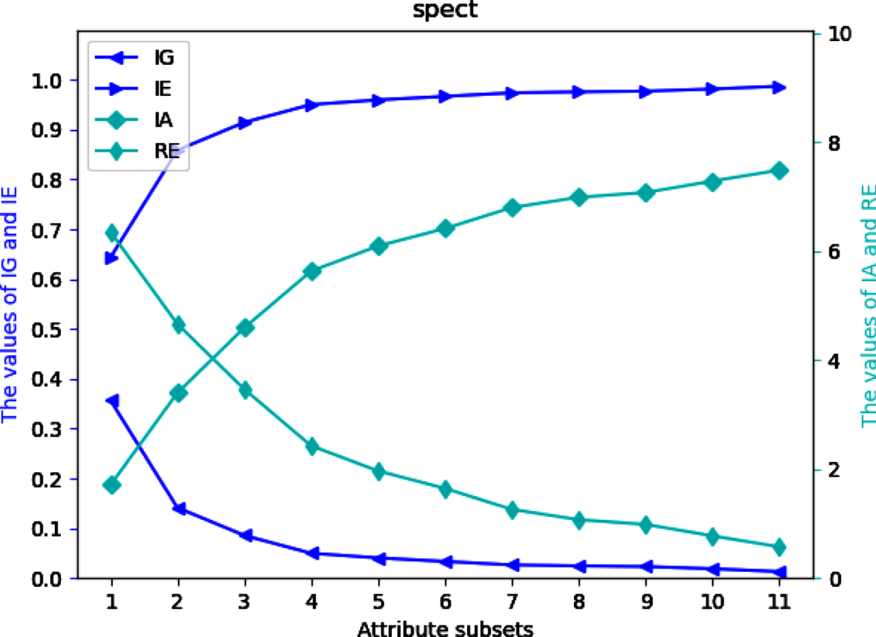
For dataset Sp, denote N_i = {a₁, ⋯ , a_2×i} (i = 1, ⋯ , 11). Then, four measurement sets of Sp are written as follows:

X_IG (Sp) = {IG (N₁) , ⋯ , IG (N₁₁)} ,

X_IE (Sp) = {IE (N₁) , ⋯ , IE (N₁₁)} ,

X_IA (Sp) = {IA (N₁) , ⋯ , IA (N₁₁)} ,

X_RE (Sp) = {RE (N₁) , ⋯ , RE (N₁₁)} .

For dataset Tt, denote O_i = {a₁, ⋯ , a_i} (i = 1, ⋯ , 9). Then, four measurement sets of Tt are written as follows:

X_IG (Tt) = {IG (O₁) , ⋯ , IG (O₉)} ,

X_IE (Tt) = {IE (O₁) , ⋯ , IE (O₉)} ,

X_IA (Tt) = {IA (O₁) , ⋯ , IA (O₉)} ,

X_RE (Tt) = {RE (O₁) , ⋯ , RE (O₉)} .

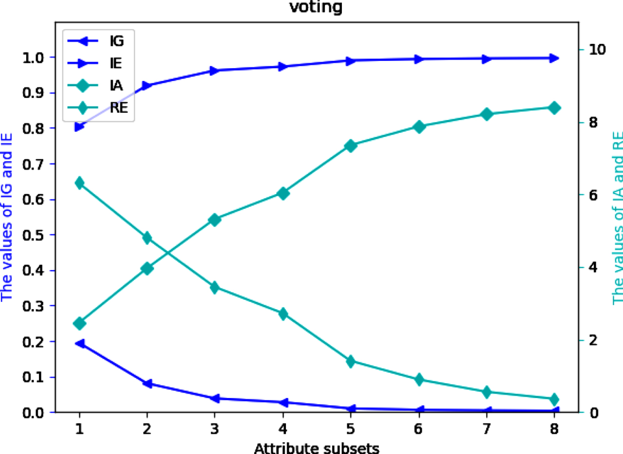
For dataset Vr, denote P_i = {a₁, ⋯ , a_2×i} (i = 1, ⋯ , 8). Then, four measurement sets of Vr are written as follows:

X_IG (Vr) = {IG (P₁) , ⋯ , IG (P₈)} ,

X_IE (Vr) = {IE (P₁) , ⋯ , IE (P₈)} ,

X_IA (Vr) = {IA (P₁) , ⋯ , IA (P₈)} ,

X_RE (Vr) = {RE (P₁) , ⋯ , RE (P₈)} .

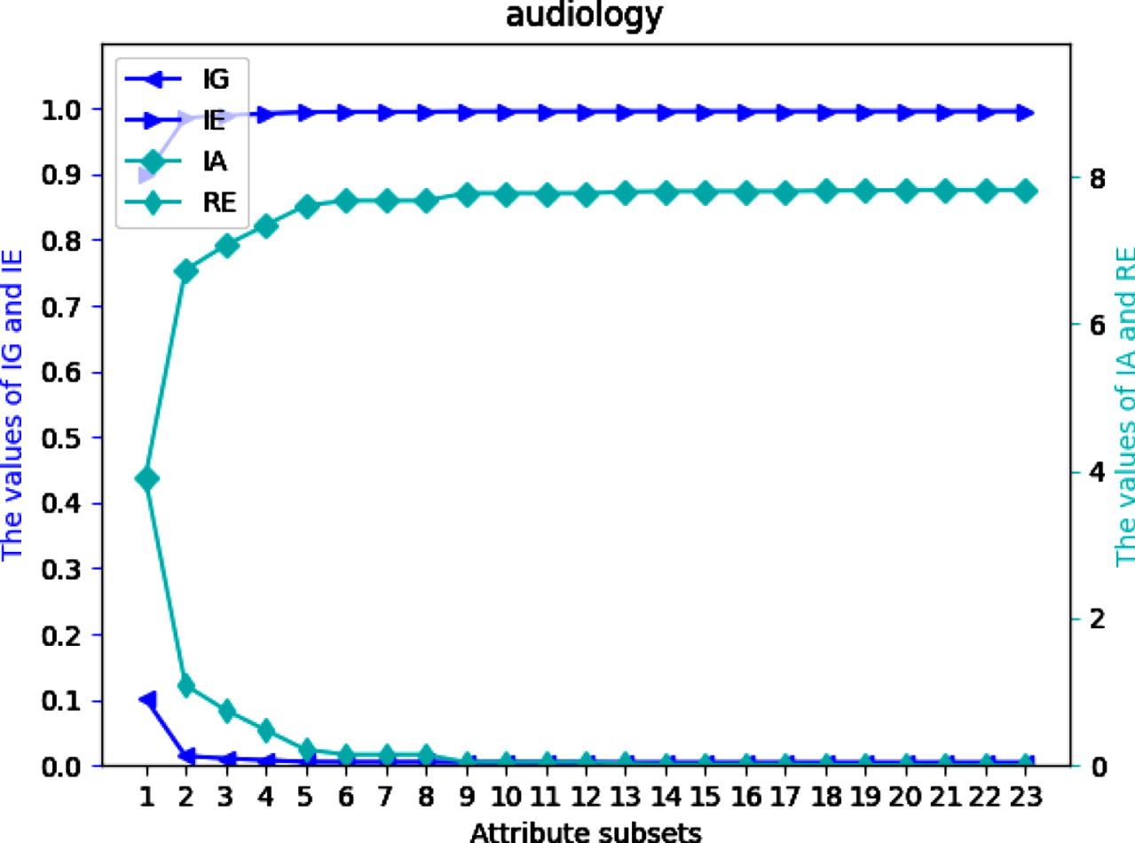
For dataset Au, denote P_i = {a₁, ⋯ , a_3×i} (i = 1, ⋯ , 23). Then, four measurement sets of Au are written as follows:

X_IG (Au) = {IG (P₁) , ⋯ , IG (P₂₃)} ,

X_IE (Au) = {IE (P₁) , ⋯ , IE (P₂₃)} ,

X_IA (Au) = {IA (P₁) , ⋯ , IA (P₂₃)} ,

X_RE (Au) = {RE (P₁) , ⋯ , RE (P₂₃)} .

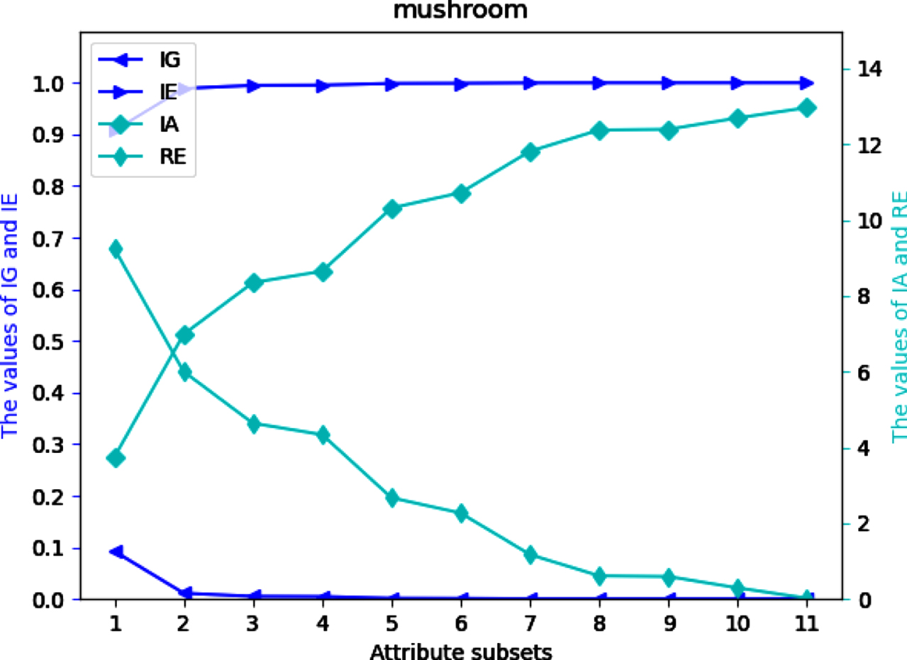
For dataset Mu, denote P_i = {a₁, ⋯ , a_2×i} (i = 1, ⋯ , 10). Then, four measurement sets of Mu are written as follows:

X_IG (Mu) = {IG (P₁) , ⋯ , IG (P₁₀)} ,

X_IE (Mu) = {IE (P₁) , ⋯ , IE (P₁₀)} ,

X_IA (Mu) = {IA (P₁) , ⋯ , IA (P₁₀)} ,

X_RE (Mu) = {RE (P₁) , ⋯ , RE (P₁₀)} .

Four UMs on each of 12 datasets are shown in Figs 2-13. The abovementioned results show that the values of IE and IA increase, when the attribute subsets become larger; Nevertheless, the values of IG and RE decrease, when the attribute subsets become larger. We can conclude that the proposed UMs in a MVIS have monotonicity with the growth of the attribute subsets. Therefore, IG, IE, IA and RE can be utilized to measure the uncertainty of a MVIS.

Fig. 2

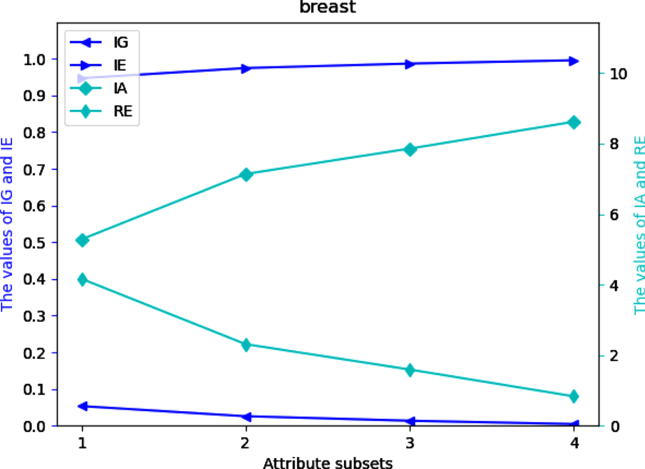
Values of IG, IE, IA and RE on dataset Br.

Fig. 3

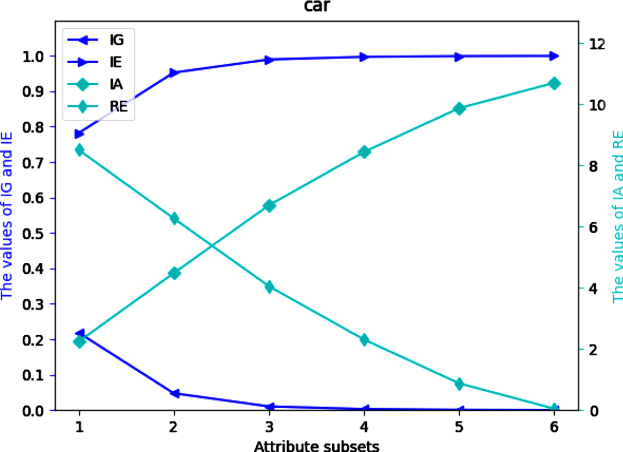
Values of IG, IE, IA and RE on dataset Ca.

Fig. 4

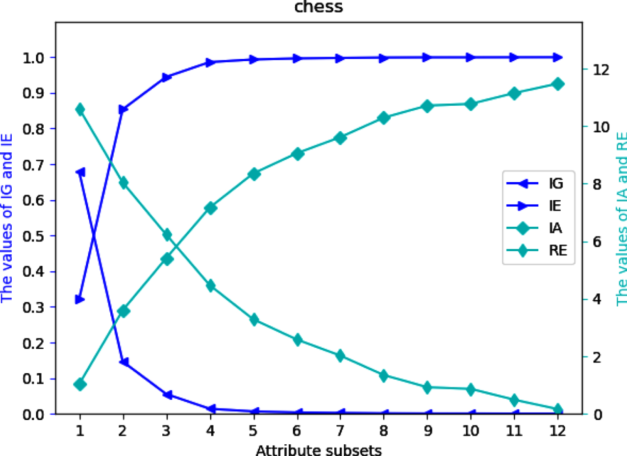
Values of IG, IE, IA and RE on dataset Ch.

Fig. 5

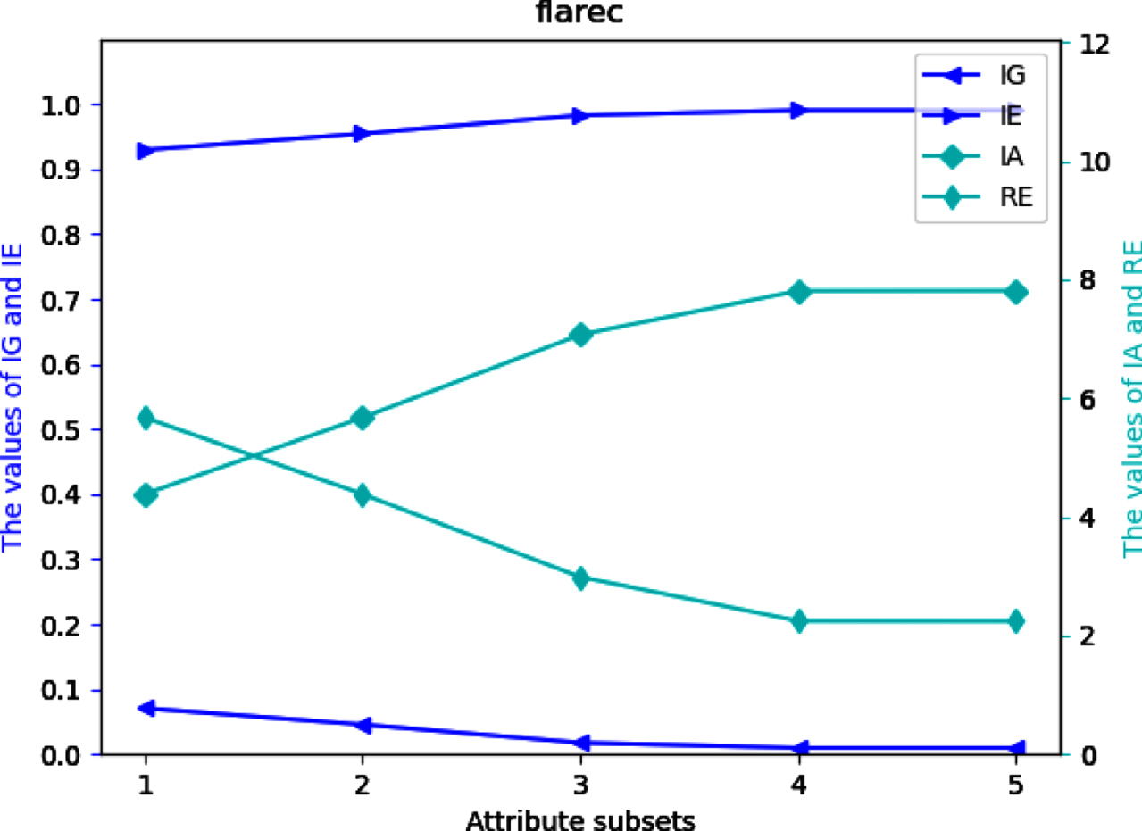
Values of IG, IE, IA and RE on dataset Fl.

Fig. 6

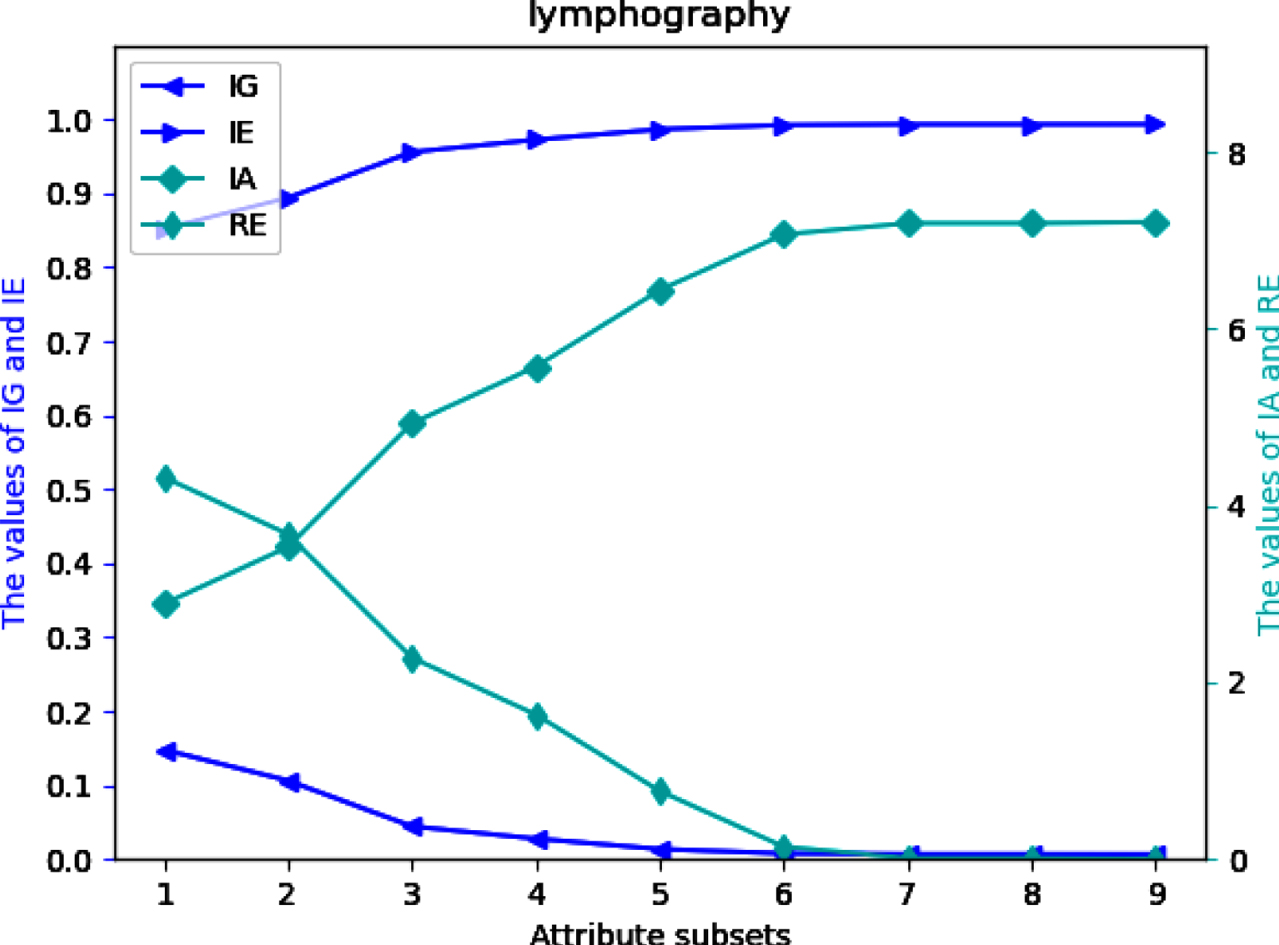
Values of IG, IE, IA and RE on dataset Ly.

Fig. 7

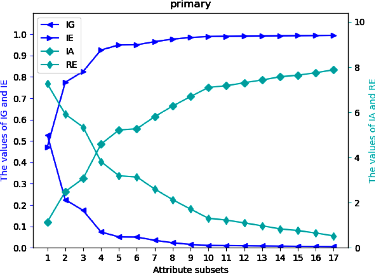
Values of IG, IE, IA and RE on dataset Pr.

Fig. 8

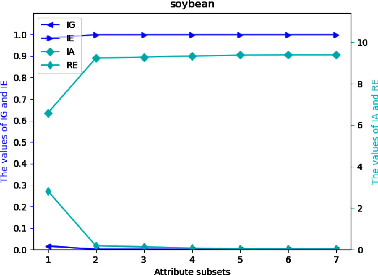
Values of IG, IE, IA and RE on dataset So.

Fig. 9

Values of IG, IE, IA and RE on dataset Sp.

Fig. 10

Values of IG, IE, IA and RE on dataset Tt.

Fig. 11

Values of IG, IE, IA and RE on dataset Vr.

Fig. 12

Values of IG, IE, IA and RE on dataset Au.

Fig. 13

Values of IG, IE, IA and RE on dataset Mu.

6.2 Dispersion analysis

In this subsection, we analyze the degree of dispersion of four UMs on the perspective of statistics.

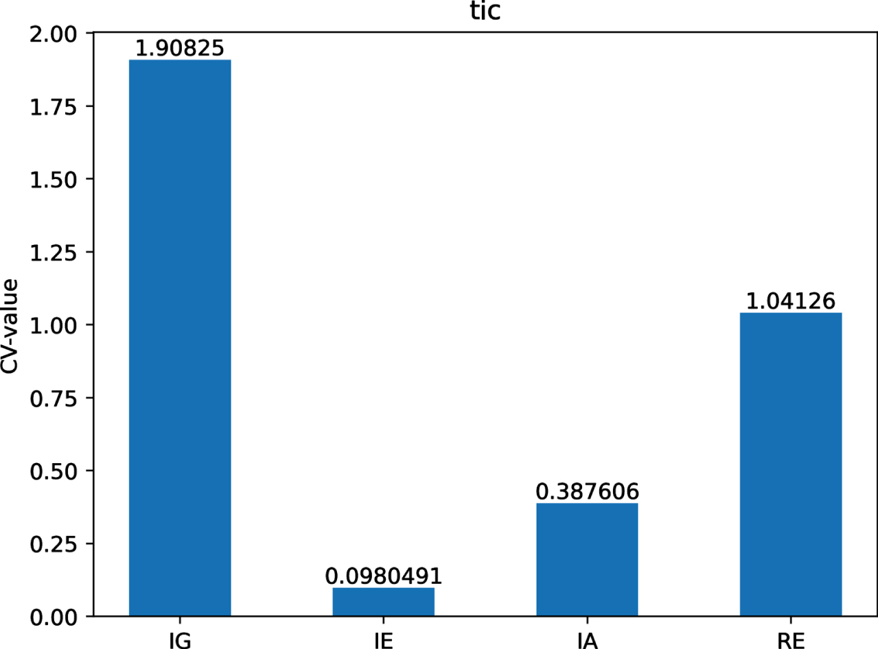
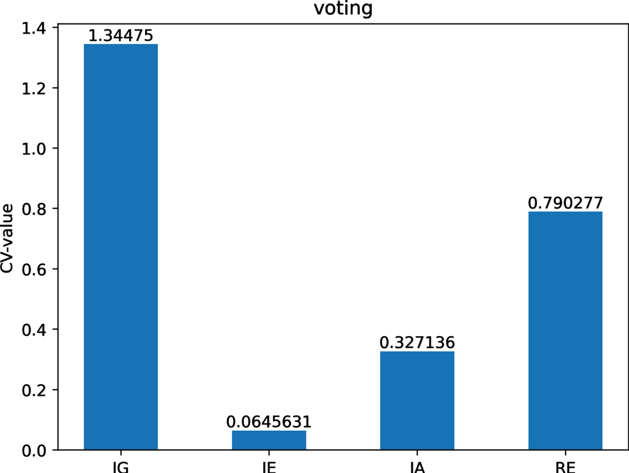
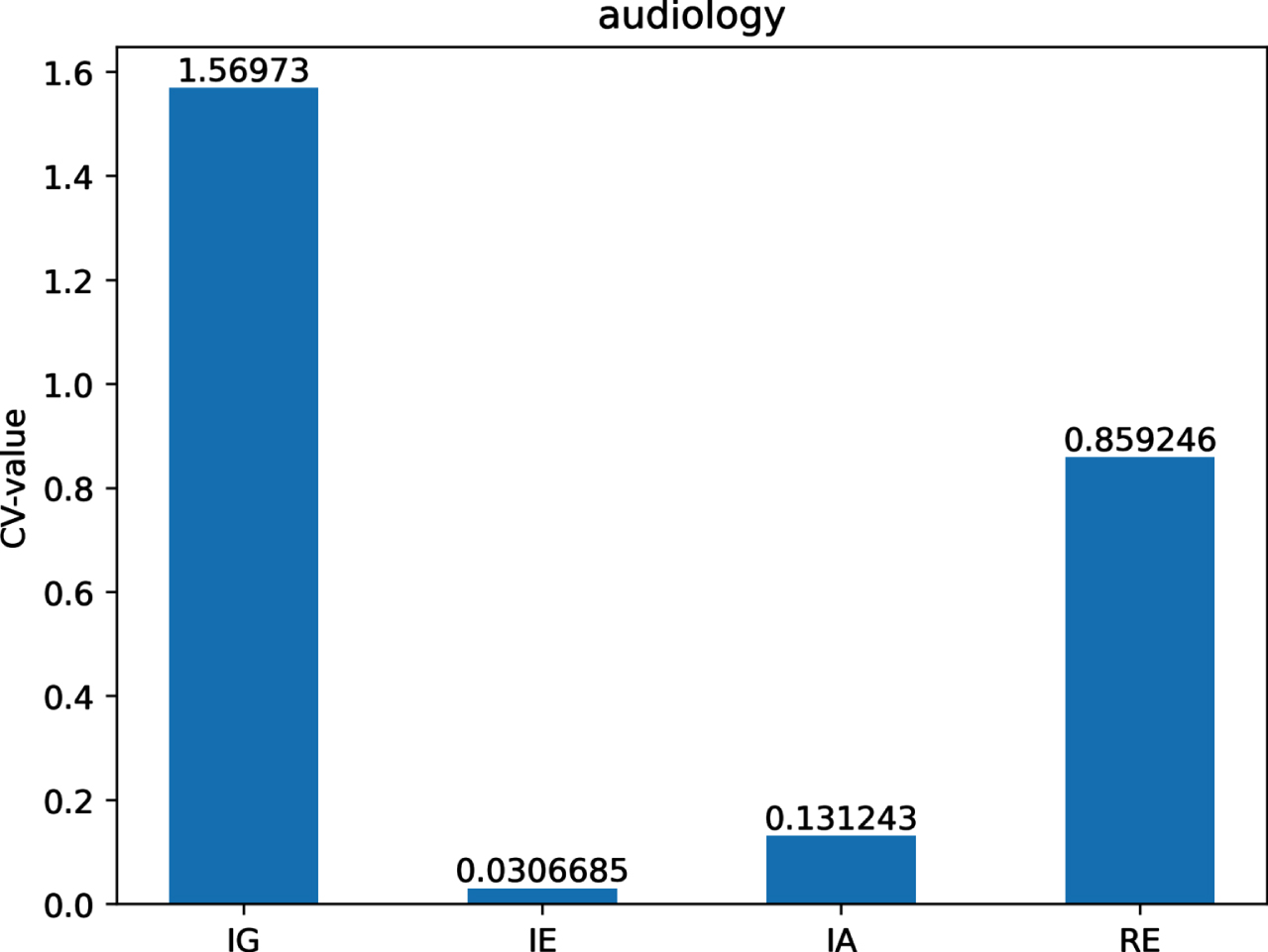
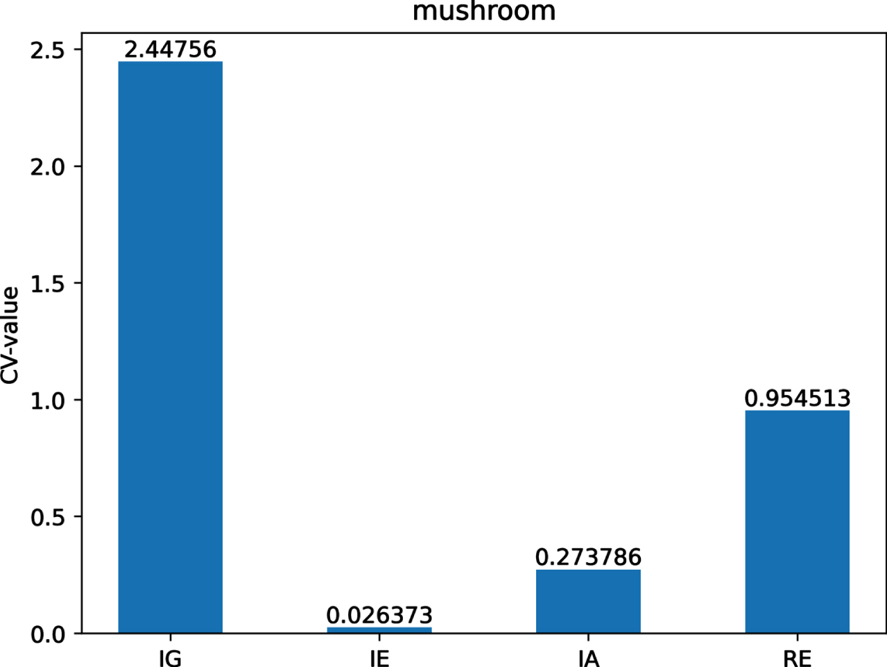
Given a dataset X = {x₁, ⋯ , x_n}, the standard deviation coefficient is defined as $CV (X) = \frac{σ (X)}{\bar{x}},$ where $\bar{x} = \frac{1}{n} \sum_{i = 1}^{n} x_{i}$ and $σ (X) = \sqrt{\frac{1}{n} \sum_{i = 1}^{n} (x_{i} - \bar{x})^{2}}$ are arithmetic average value and standard deviation of X, respectively.

In the following expressions, standard deviation coefficient is referred to as CV-value.

The standard deviation coefficient can represent the degree of dispersion between datasets, the larger standard deviation coefficient is, the higher dispersion is; the smaller standard deviation coefficient is, the lower dispersion is.

With that in mind, we can compute the CV-values of IG, IE, IA and RE on each of twelve datasets are shown in Figs 12-21.

Fig. 14

The CV-values of IG, IE, IA and RE on dataset Br.

Fig. 15

The CV-values of IG, IE, IA and RE on dataset Ca.

Fig. 16

The CV-values of IG, IE, IA and RE on dataset Ch.

Fig. 17

The CV-values of IG, IE, IA and RE on dataset Fl.

Fig. 18

The CV-values of IG, IE, IA and RE on dataset Ly.

Fig. 19

The CV-values of IG, IE, IA and RE on dataset Pr.

Fig. 20

The CV-values of IG, IE, IA and RE on dataset So.

Fig. 21

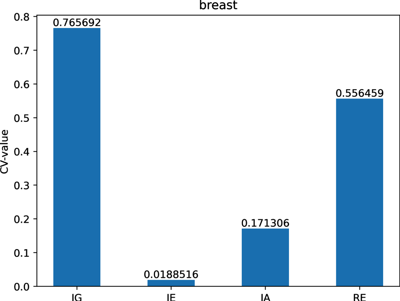
The CV-values of IG, IE, IA and RE on dataset Sp.

Fig. 22

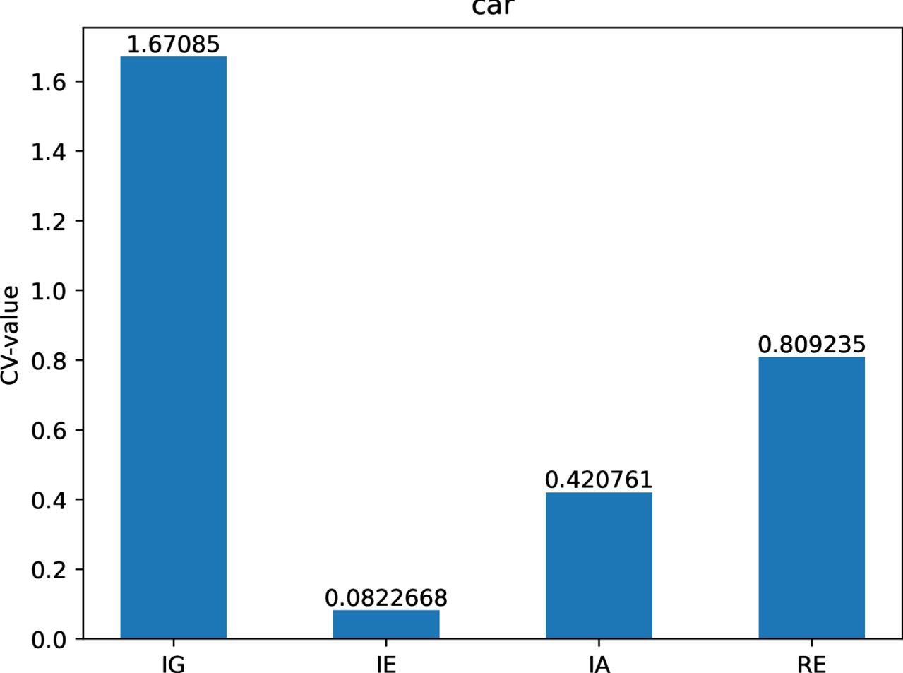
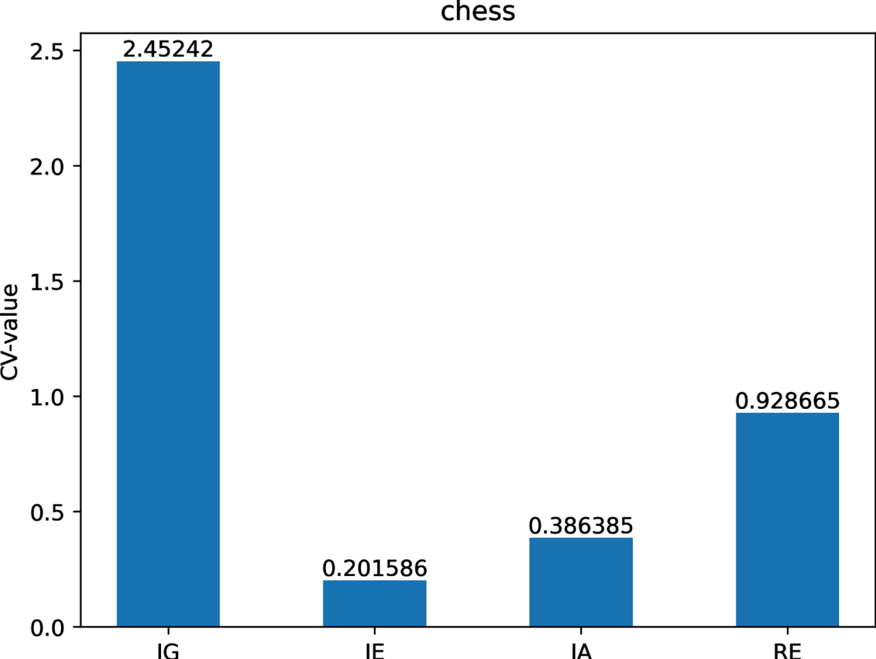
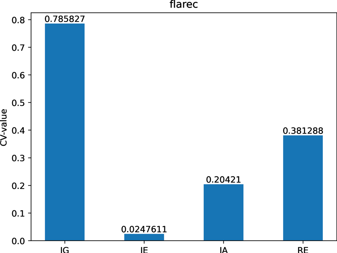
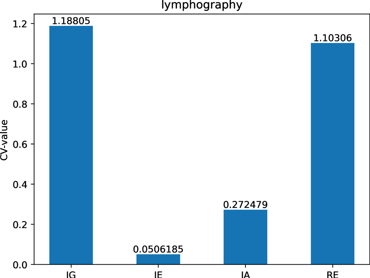
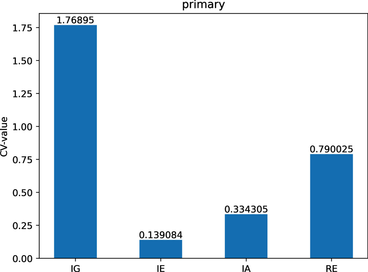
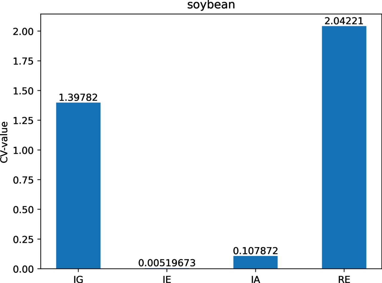
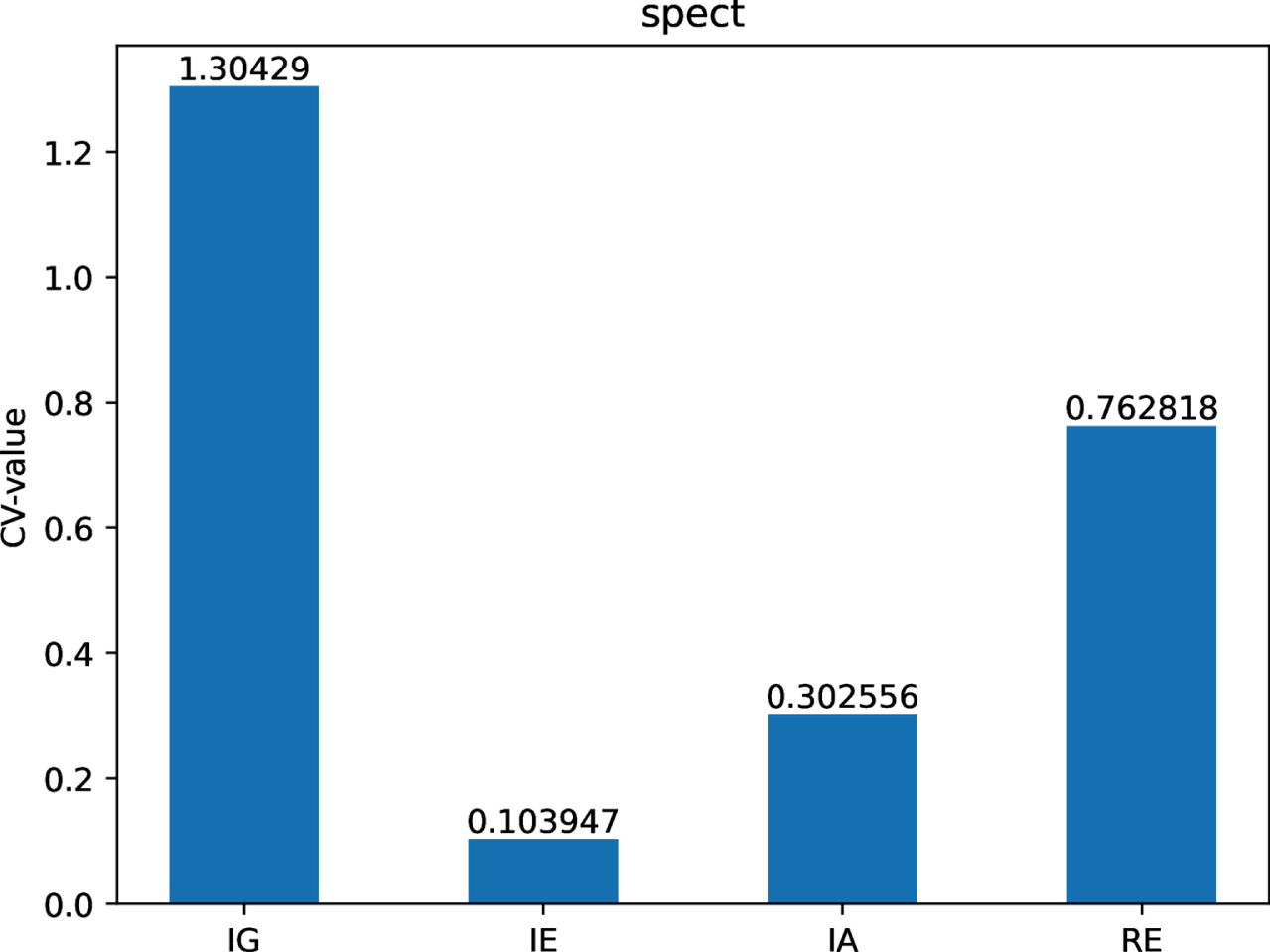
The CV-values of IG, IE, IA and RE on dataset Tt.

Fig. 23

The CV-values of IG, IE, IA and RE on dataset Vr.

Fig. 24

The CV-values of IG, IE, IA and RE on dataset Au.

Fig. 25

The CV-values of IG, IE, IA and RE on dataset Mu.

Figs 12-21 indicate that the CV-values of IG and RE are much greater than those of IE and IA on each of twelve datasets. Therefore, IE and IA have the best measuring effect on the uncertainty of twelve datasets. In other words, IE and IA are more suitable for measuring the uncertainty of a MVIS from the perspective of dispersion.

6.3 Friedman test and Nemenyi test

Friedman test is a statistical test, which is usually used to compare the overall performance of k algorithms on N datasets. If there were different performances, the Nemenyi test will be applied to distinguish which algorithm is significantly different from other algorithms. In this subsection, we will use Friedman test and Nemenyi test to demonstrate which uncertainty measurement has better performance.

Suppose that N and k are the number of datasets and algorithms, respectively. The Friedman test is defined by $τ_{F} = \frac{(N - 1) τ_{χ^{2}}}{N (k - 1) - τ_{χ^{2}}},$ where $τ_{χ^{2}} = \frac{12 N}{k (k + 1)} \sum_{i = 1}^{k} r_{i}^{2} - 3 N (k + 1)$ and r_i represents the average ranking of the i-th (i = 1, 2, ⋯ , k) algorithm.

τ_F is the F-distribution with k - 1 and (k - 1) (N - 1) degrees of freedom. If the value of τ_F is greater than τ_α (k - 1, (k - 1) (N - 1)), then null hypothesis is rejected. It indicates that there is a significant difference between algorithms, then we can continue to carry out the Nemenyi test.

The Nemenyi test of critical difference, written as CD_α, is defined by ${CD}_{α} = q_{α} \sqrt{\frac{k (k + 1)}{6 N}},$ where q_α is the critical value and α is the significance level. If the difference between average ranking of each pair of algorithms is greater than CD_α, it indicates that there is a significant difference between the pair of algorithms; otherwise, there is no significant difference between the pair of algorithms.

In subection 6.2, the CV-values of IG, IE, IA and RE on each of twelve datasets are received and showed in Table 10. Four UMs can be regarded as four algorithms and ranked by CV-values on each of twelve datasets. The results of the ranking of CV-values are depicted in Table 11.

Table 10
The CV-values of IG, IE, IA and RE on each of twelve datasets

Datasets IG IE IA RE

Br 0.7657 0.0189 0.1713 0.5565

Ca 1.6709 0.0823 0.4208 0.8092

Ch 2.4524 0.2016 0.3864 0.9287

Fl 0.7858 0.0248 0.2042 0.3813

Ly 1.1881 0.0507 0.2725 1.1031

Pr 1.7689 0.1391 0.3343 0.7900

So 1.3978 0.0052 0.1079 2.0422

Sp 1.3043 0.1039 0.3026 0.7628

Tt 1.9083 0.0980 0.3876 1.0412

Vr 1.3448 0.0646 0.3271 0.7903

Au 1.5697 0.0307 0.1312 0.8592

Mu 2.4476 0.0264 0.2738 0.9545

Datasets	IG	IE	IA	RE
Br	0.7657	0.0189	0.1713	0.5565
Ca	1.6709	0.0823	0.4208	0.8092
Ch	2.4524	0.2016	0.3864	0.9287
Fl	0.7858	0.0248	0.2042	0.3813
Ly	1.1881	0.0507	0.2725	1.1031
Pr	1.7689	0.1391	0.3343	0.7900
So	1.3978	0.0052	0.1079	2.0422
Sp	1.3043	0.1039	0.3026	0.7628
Tt	1.9083	0.0980	0.3876	1.0412
Vr	1.3448	0.0646	0.3271	0.7903
Au	1.5697	0.0307	0.1312	0.8592
Mu	2.4476	0.0264	0.2738	0.9545

Table 11

The ranking of CV-values of IG, IE, IA and RE on each of twelve datasets

Datasets	IG	IE	IA	RE
Br	4	1	2	3
Ca	4	1	2	3
Ch	4	1	2	3
Fl	4	1	2	3
Ly	4	1	2	3
Pr	4	1	2	3
So	3	1	2	4
Sp	4	1	2	3
Tt	4	1	2	3
Vr	4	1	2	3
Au	4	1	2	3
Mu	4	1	2	3
Average	3.9	1	2	3.1

In the following, Friedman test and Nemenyi test will be used to test the performance of four UMs.

(1) For twelve datasets and four UMs, τ_F is the F-distribution with 3 and 33 degrees of freedom. We can calculate τ_0.05 (3, 33) =2.89, τ_F = 294.56. Apparently, τ_F is much larger than 2.96. Hence, the null hypothesis is rejected under the significance level α = 0.05, namely, IG, IE, IA and RE have dramatic difference on performance.

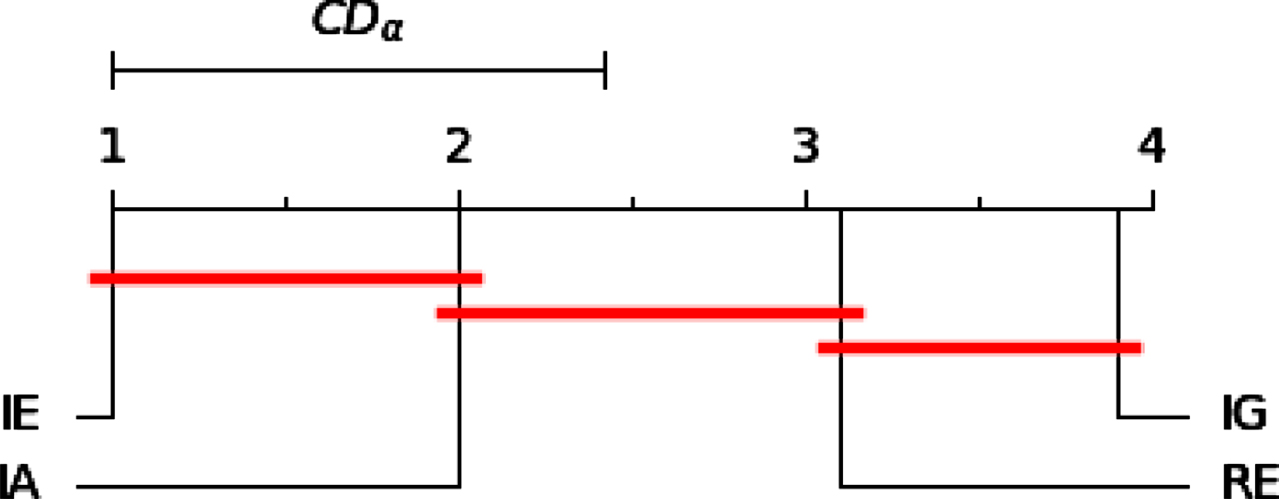
(2) To further demonstrate the dramatic difference between any two of IG, IE, IA and RE, the Nemenyi test is carried out. After calculation, ${CD}_{α} = 2.569 \times \sqrt{\frac{4 \times (4 + 1)}{6 \times 12}} = 1.354$ under the significance level α = 0.05. Fig 26 reveals the results of the Nemenyi test for four UMs under the significance level α = 0.05.

Fig. 26

The results of the Nemenyi test for four UMs.

From Fig 26, we can draw the following conclusions:

(i) IE is statistically superior to other UMs, namely, IE has better performance than other UMs.

(ii) There is significant difference between IE and RE, IE and IG, and IA and IG.

(iii) There is no significant difference between IE and IA, IA and RE, IG and RE.

6.4 Comparisons

1) In information systems, uncertain data are often presented in fuzzy form. Liu et al. [20] studied measures of uncertainty based on Gaussian kernel for type-2 fuzzy information systems, they are δ-coarse granularity and δ-rough entropy. Through effectiveness analysis, δ-coarse granularity and δ-rough entropy are monotonically decreasing when attribute subset become larger. It means that when the attribute subset becomes larger, the uncertainty of type-2 fuzzy information system is reduced.

2) Considering that relatively less studies for the interval-valued decision systems, Liao et al. [26] proposed three-level and three-way uncertainty measurements by means of three-way weighted entropies of interval-valued decision systems. Through theoretically deduced and experimentally verified three-level and three-way uncertainty measurements are monotonicity and non-monotonicity, respectively.

3) A MVIS can be seen as a model that is the result of information fusion of multiple categorical ISs and helps deal with missing values in the dataset. This paper constructs information structures in a MVIS based on tolerance relations by using set matrices. On the basis of the information structures, granularity measures, entropy measures and information amounts are proposed to measure uncertainty of a MVIS. Through theoretically deduced and experimentally illustrate that the proposed measures are monotonicity.

7 Conclusions

In this paper, information structures in a MVIS have been proposed and studied. Actually, information structures were composed of information granules from the view of GrC. Information granules have been constructed from tolerance relations by means of Hellinger distance in a MVIS. The family of all these information granules constitutes a vector that is a information structure induced by a given attribute subset. Considering the association of information structures induced by two attribute subsets, relationships between information structures have been researched from two aspects of dependence and separation. In addition, some properties of information structures by using information distance and inclusion degree have been proved. Uncertainty measurements as the applications of information structure have been investigated, numerical experiments and effectiveness analysis on twelve datasets demonstrate the uncertainty measurement of IE that had better performance than others. Nevertheless, the proposed four UMs of a MVIS only are the extension of the previous measurement index and we do not consider how to more effectively choose the parameter θ. In future work, we will study how to more effectively choose parameter θ in practical application and use information structures to deal with decision making problems under uncertainty.

Footnotes

Acknowledgments

The authors would like to thank the editors and the anonymous reviewers for their valuable comments and suggestions which have helped immensely in improving the quality of this paper. This work is supported by Guangxi university middle-aged and young teachers’ basic scientific research ability improvement project(2020KY19012).

References

Blizard

W.D.

, Multiset theory, Notre Dame Journal of FormalLogic 30 (1989), 36–66.

Bar-Shalom

and Fortman

, Tracking and Data Association, The Journal of the Acoustical Society of America 87 (1990), 918–919.

Barbara

, Garcia-Molina

, Porter

A probabilistic relational data model, (1990).

Barbara

, Garcia-Molina

and Porter

, The management ofprobabilistic data, IEEE Transactions on Knowledge & DataEngineering 4 (1992), 487–502.

Boekowski

, Peters

J.F.

Approximating sensor signals: A rough set approachcčňElectrical and Computer Engineering (2002), 980–985.

Chan

C.C.

, Rough set approach to attribute generalization in datamining, Information Science 107 (1998), 169–176.

Chmielewski

M.R.

and Grzymala-Busse

J.M.

, Global discretization ofcontinuous attributes as preprocessing for machine learning, International Journal of Approximate Reasoning 15 (1996), 319–331.

Cament

L.A.

, Castillo

L.E.

, Perez

J.P.

and Galdames

F.J.

, and C.A.Perez, Fusion of local normalization and Gabor entropy weightedfeatures for face identifification, Pattern Recognition 47 (2014), 568–577.

Chen

N.P.

and Qin

, Invariant characterizations of informationstructures in a lattice-valued information system underhomomorphisms based on data compression, Journal of Intelligent& Fuzzy Systems 33 (2017), 3987–3998.

10.

Dempster

A.P.

, Upper and lower probabilities induced by amultivalued mapping, Annals of Mathematical Statistics 38 (1967), 325–339.

11.

Dai

J.H.

and Tian

H.W.

, Entropy measures and granularity measuresfor set-valued information systems, Information Sciences 240 (2013), 72–82.

12.

Guan

, Zhen

Consensus reaching with non-cooperative behavior management for personalized individual semantics-based social network group decision making, Journal of the Operational Research Society, https://doi.org/10.1080/01605682.2021.1997654.

13.

Hou

W.J.

, Li

X.J.

, Jin

, Wu

neural networks and expert system, International Conference Cyber worlds (2008), 811–814.

14.

Huang

Y.Y.

, Li

T.R.

, Luo

and Wang

, Dynamic fusion ofmulti-source interval-valued data by fuzzy granulation, IEEETransactions of Fuzzy Systems 26 (2018), 3403–3417.

15.

Hempelmann

C.F.

, Sakoglu

, Gurupur

V.P.

and Jampana

, Anentropy-based evaluation method for knowledge bases of medicalinformation systems, Expert Systems with Applications 46(2016), 262–273.

16.

Kim

, Data classification based on tolerant rough set, Patterm Recognition 34 (2001), 1613–1624.

17.

Lin

Generalized metric spaces and mappings, Chinese Scientific Publishers, Beijing 1995.

18.

Liu

, Application of granular and granular computing in logicalreasoning, Computer Research and Development 41 (2004), 546–551.

19.

Lin

T.Y.

Granular computing on binary relations I: data mining and neighborhood systems, Rough Sets In Snowledge Discovery (1998), 107–121.

20.

Liu

X.F.

, Dai

J.H.

and Chen

J.L.

, C.Z.Wang and J.M. Zhan, Measures ofUncertainty Based on Gaussian Kernel for Type-2 Fuzzy InformationSystems, International Journal of Fuzzy Systems 23(2021), 1163–1178.

21.

Liucň

, Sun

Wang

H.F.

, Research status of granular computing and granular computing based on rough logic semantics, Journal of Computer Science 31 (2008), 543–555.

22.

Liang

J.Y.

and Shi

Z.Z.

, The information entropy, rough entropy andknowledge granulation in rough set theory, InternationalJournal of Uncertainty, Fuzziness and Knowledge-Based Systems 12 (2004), 37–46.

23.

Liang

J.Y.

, Shi

Z.Z.

, Li

D.Y.

and Wierman

M.J.

, The informationentropy, rough entropy and knowledge granulation in incompleteinformation systems, International Journal of General Systems 35 (2006), 641–654.

24.

Liang

J.Y.

and Qian

Y.H.

, Information Granules and Entropy Theory inInformation Systems, Information Sciences 51 (2008), 1427–1444.

25.

M.M.

and Wang

X.Z.

, Information fusion based on informationentropy in fuzzy multi-source incomplete information system, International Journal of Fuzzy Systems 19 (2017), 1200–1216.

26.

Liao

S.J.

, Zhang

X.Y.

and Mo

Z.W.

, Three-level and three-wayuncertainty measurements for interval-valued decision systems, International Journal of Machine Learning and Cybernetics 12(2021), 1–23.

27.

Khan

M.A.

and Banerjee

, Formal reasoning with rough sets inmultiple-source approximation systems, International Journal ofApproximate Reasoning 49 (2008), 466–477.

28.

Mssherry

, Knowledge discovery by inspection, DecisionSupport Systems 21 (1997), 43–37.

29.

Miao

D.Q.

, Wang

G.Y.

, Liu

, Lin

T.Y.

, Yao

Y.Y.

Granular computing: past, present and future prospect, Science Press, Beijing, 2007.

30.

Miao

Q.D.

and Wang

, On the relationships between informationentropy and roughness of konwledge in rough set theory, PatternRecognition and Aitificial Intelligence 11 (1998), 34–40.

31.

Navarrete

, Viejo

and Cazorla

, Color smoothing for RGB-Ddata using entropy information, Applied Soft Computing 46 (2016), 380.

32.

Xie

N.X.

, Li

Z.W.

, Zhang

P.F.

and Zhang

G.Q.

, Information structuresand uncertainty measures in an incomplete probabilistic set-valuedinformation system, IEEE Access 7 (2019), 27501–27514.

33.

W.H.

, Zhang

X.Y.

and Zhang

W.X.

, Knowledge granulation, knowledgeentropy and knowledge uncertainty measure in ordered informationsystems, Applied Soft Computing 9 (2009), 1244–1251.

34.

Pawlak

, Rough sets, International Journal of Computer andInformation Science 11 (1982), 341–356.

35.

Pawlak

and Skowron

, Rough sets and boolean reasoning, Infomation Sciences 177 (2007), 41–73.

36.

Pawlak

and Skowron

, Rudiments of rough sets, InformationSciences 177 (2007), 3–27.

37.

Pawlak

Dordrecht: Kluwer Academic Publishers, (1991), 45–64.

38.

Pavlin

, Patrick

, Maris

, Nunnink

and Hood

, Amulti-agent systems approach to distributed bayesian informationfusion, Information Fusion 11 (2010), 267–282.

39.

Qian

Y.H.

, Liang

J.Y.

and Dang

C.Y.

, Knowledge Structure, Knowledgegranulation and knowledge ditance in a knowledge base, International Journal of Approximate Reasoning 50 (2009), 174–188.

40.

Qian

H.Y.

and Liang

Y.J.

, Combination entropy and combinationgranulation in rough set theory, International Journal ofUncertainty, Fuzziness and Knowledge-Based System 16(2008), 179–193.

41.

Ristic

, Gilliam

and Byrne

, Performance assessment of asystem for reasoning under uncertainty in information fusion, Information Fusion 71 (2021), 11–16.

42.

Solaiman

, Piercecň

L.E.

and Ulaby

F.T.

, Multisensor datafusion using fuzzy concepts: application to land-coverclassification using ERS-1/JERS-1 SAR composites, IEEETransaction on Geosciences and Remote Sensing 37 (1999), 1316–1326.

43.

The URL of UCI datasets: http://archive.ics.uci.edu/ml/datasets.php.

44.

Wei

and Liang

J.Y.

, Information fusion in rough set theory: anoverview, Information Fusion 48 (2019), 107–118.

45.

Xie

S.D.

and Wang

Y.X.

, Construction of tree network with limiteddelivery latency in homogeneous wireless sensor networks, Wireless Personal Communications 78 (2014), 231–246.

46.

W.H.

and Yu

J.H.

, A novel approach to information fusion inmulti-source datasets: A granular computing viewpoint, Information Sciences 378 (2017), 410–423.

47.

Yao

Y.Y.

, Infomation granulation and rough set approximation, Lintermatonal Joural of Intelligent Systems 16 (2001), 87–104.

48.

G.J.

, Information structures in an incomplete information system:A granular computing viewpoint, International Journal ofComputational Intelligence Systems 11 (2018), 11–79.

49.

Yao

Y.Y.

, A partition model of granular computing, LNCSTransactions on Rough Sets I (2004), 232–253.

50.

Zadeh

L.A.

, Fuzzy logic equals computing with words, IEEETransactions Fuzzy Systems 4 (1996), 103–111.

51.

Zadeh

L.A.

, Toward a theory of fuzzy information granulation and itscentrality in human reasoning and fuzzy logic, Fuzzy Sets andSystems 90 (1997), 111–127.

52.

Zhang

G.Q.

, Li

Z.W.

, Wu

W.Z.

, Liu

X.F.

and Xie

N.X.

, Informationstructures and uncertainty measuresin a fully fuzzy informationsystem, International Jourmal of Approximate Reasoning 101 (2018), 119–149.

53.

Zhang

, L

Z.L.

Personalized individual semantics based consistency control and consensus reaching 1140 in linguistic group decision making, IEEE transactions on systems, man, and cybernetics: systems, https://doi.org/10.1109/TSMC.2021.3129510.

54.

Zhang

Y.P.

, Zhang

and Wu

, The Representation of DifferentGramular Worlds: A Quotient Space, Chinese Jourmal OfComputers 27 (2004), 328–333.

Information structures in a multiset-valued information system with application to uncertainty measurement

Abstract

Keywords

1 Introduction

1.1 Background and related work

1.2 Motivation and inspiration

1.3 Organization

2.1 Binary relations

2.2 Multisets

2.3 Probability distribution sets

2.4 Relationships between multisets and PDSs

3 Multiset-valued information systems

3.1 The concept of multiset-valued information system

Table 1 An IIS about cars O a 1 a 2 a 3 a 4 o 1 L C * L o 2 H F D H o 3 L F * H o 4 L C D M o 5 H * * M o 6 H C G * o 7 L F G L o 8 H * D H o 9 L C D L

4 Information structures in a MVIS

4.1 The concept of information structures in a MVIS

4.2 Relationships between information structures in a MVIS

4.2.1 Dependence between information structures in a MVIS

4.2.2 Information distance between information structures in a MVIS

5 Uncertainty measurement of a MVIS

5.1 Information granulation of a MVIS

5.2 Information entropy of a MVIS

5.3 Information amount of a MVIS

5.4 Rough entropy of a MVIS

6 Numerical experiments and effectiveness analysis

6.1 Numericals experiment

7 Conclusions

Footnotes

Acknowledgments

References

Table 1
An IIS about cars

O a ₁ a ₂ a ₃ a ₄

o ₁ L C * L

o ₂ H F D H

o ₃ L F * H

o ₄ L C D M

o ₅ H * * M

o ₆ H C G *

o ₇ L F G L

o ₈ H * D H

o ₉ L C D L