A novel adaptive boundary weighted and synthetic minority oversampling algorithm for imbalanced datasets

Abstract

In recent years, imbalanced data learning has attracted a lot of attention from academia and industry as a new challenge. In order to solve the problems such as imbalances between and within classes, this paper proposes an adaptive boundary weighted synthetic minority oversampling algorithm (ABWSMO) for unbalanced datasets. ABWSMO calculates the sample space clustering density based on the distribution of the underlying data and the K-Means clustering algorithm, incorporates local weighting strategies and global weighting strategies to improve the SMOTE algorithm to generate data mechanisms that enhance the learning of important samples at the boundary of unbalanced data sets and avoid the traditional oversampling algorithm generate unnecessary noise. The effectiveness of this sampling algorithm in improving data imbalance is verified by experimentally comparing five traditional oversampling algorithms on 16 unbalanced ratio datasets and 3 classifiers in the UCI database.

Keywords

Imbalanced data oversampling classifier boundary weighted within and between class imbalance

1 Introduction

The classification issue is one of the important research topics in the field of machine learning. Traditional classification methods have achieved good results and accuracy in classifying balanced datasets [13, 18]. However, real datasets are often unbalanced. Imbalance in the data is manifested in two main ways, one is imbalance between classes, that is, the difference between the sample size of one class and the sample size of another class. In addition to imbalances between the majority class and the minority sample, imbalances can also occur within a class of samples. For example, in a common dataset in medicine, an unbalanced medical dataset has ‘healthy’ as the majority sample and ‘sick’ as the minority sample. However, in the ‘sick’ category, the number of leukaemia patients is certainly much smaller than the number of flu patients. For example, an unbalanced medical dataset in a medically common dataset has ‘healthy’ as the majority sample and ‘sick’ as the minority sample. However, in the ‘sick’ category, the number of leukaemia patients is certainly much smaller than the number of flu patients. The dataset mentioned above is the unbalanced dataset that contains between-classes and within-classes at the same time.

In general, techniques for improving unbalanced data are divided into algorithm-level methods, data-level methods [26]. At the level of classification algorithm, the commonly used methods include cost-sensitive learning, single classifier method and ensemble learning method [30]. At the data level, some strategies are adopted to change the distribution of samples and transform unbalanced samples into a state of relatively balanced distribution [24]. The sampling of training data can be accomplished by removing majority samples (under-sampling) or adding minority samples (over-sampling). However, under-sampling runs the risk of losing important samples. Random over-sampling randomly repeats the minority samples until a balanced distribution of samples is reached. It is the most commonly used of the over-sampling methods because it is simple and easy to implement [29]. However, since the sample is simply repeated, classifiers trained on random over-sampled data can be overfitted.

Chawla et al. suggested the SMOTE algorithm, which avoids the risk of overfitting faced by random over-sampling [7]. Based on the SMOTE algorithm, many classic algorithms were born. Borderline-SMOTE1 changes the random sample selection strategy of SMOTE and focuses on generating minority samples at the decision boundary. This approach resolves the between class imbalance but not the within class imbalance, and also tends to create the problem of missing important samples [15]. Proposed method in this paper addresses the imbalance problem of between and within class, while avoiding the problem of important samples loss that arises with this approach. Borderline-SMOTE2 extends Borderline-SMOTE1 to allow interpolation between a minority sample and one of its majority samples nearest neighbors by setting the interpolation weight to less than 0.5, thus making the generated sample closer to the minority sample. However, this method also have the problem of missing important samples. Cluster-SMOTE combines an over-sampling algorithm with a clustering algorithm, using K-means to cluster minority samples and then applying SMOTE to the clusters [1]. While this approach solves the problem of within-class imbalance, it does not specify how many samples to generate in each cluster or how to determine the optimal number of samples. Our proposed method solves this problem by determining the number of samples per cluster and boundary through a strategy of determining global sample weights and local sample weights. In recent years, Alejot et al. proposed the neural network method in deep learning to improve the learning of imbalanced data. This algorithm solves the classification of unbalanced data under a large number of data [2]. Compared with the method proposed in this paper, the above method has high complexity and poor classification effect on small data sets. Jz A et al. proposed a weighted hybrid ensemble method to classify unbalanced data, in which each sampling method and each classifier are assigned corresponding weights, addressing only the within-class imbalance. The two weight assignment strategies used in the proposed method address inter-class imbalance and intra-class imbalance more precisely than the method [19]. Aurelio et al. used a weighted cross-entropy function to solve the data imbalance problem of the target dataset. Compared with the method proposed in this paper, the algorithm is more expensive to learn and the efficiency of the algorithm needs to be improved [3]. Jerzy et al, proposed A domain-based feature learning method for local data to change the imbalanced data and improve the classification results, but it is blind to the overlapping class boundaries, so it may lead to noise [6]. The method proposed in this paper can effectively avoid the generation of noisy samples and improve the accuracy of the classifier. Asniar et al. proposed a method to improve the SMOTE algorithm by adding a local outlier factor (LOF), while the ABWSMO algorithm combines the SMOTE algorithm with the K-Means clustering algorithm to generate minority class samples, improving the classification accuracy and the generalisation capability of the algorithm [5]. Ssa B et all. propose a generative adversarial network to enhance the quality of generated minority class samples. The method proposed in this paper has higher classifier accuracy than this approach and is applicable to a wider range of datasets [28].

In this paper, we proposed A Novel Adaptive Boundary Weighted and Synthetic Minority Oversampling Algorithm for Imbalanced Datasets (ABWSMO). ABWSMO proposes two innovative weight determination strategies, an adaptive boundary adjustment strategy and an adaptive oversampling sample size determination strategy. And these two strategies are cleverly combined with the improved SMOTE algorithm and K-means algorithm to effectively overcome the shortcomings of traditional oversampling algorithms. The proposed method eliminates the within-class and between-class imbalance, avoids the generation of noise samples, balances the minority and majority samples, and enhances the learning of boundary samples, thus improving the classification performance of the classifier.

2 Related theory

2.1 SMOTE algorithm

The SMOTE algorithm, which avoids the risk of overfitting faced by random oversampling [16]. As shown in Fig. 1, SMOTE generates a new sample by randomly selecting a minority sample and linearly interpolating among its k nearest minority samples. More precisely, SMOTE executes three steps to generate a new minority class sample [21].

It selects a random minority sample $\tilde{a}$ observe.

Among its k nearest minority samples neighbors, instance $\tilde{b}$ is selected.

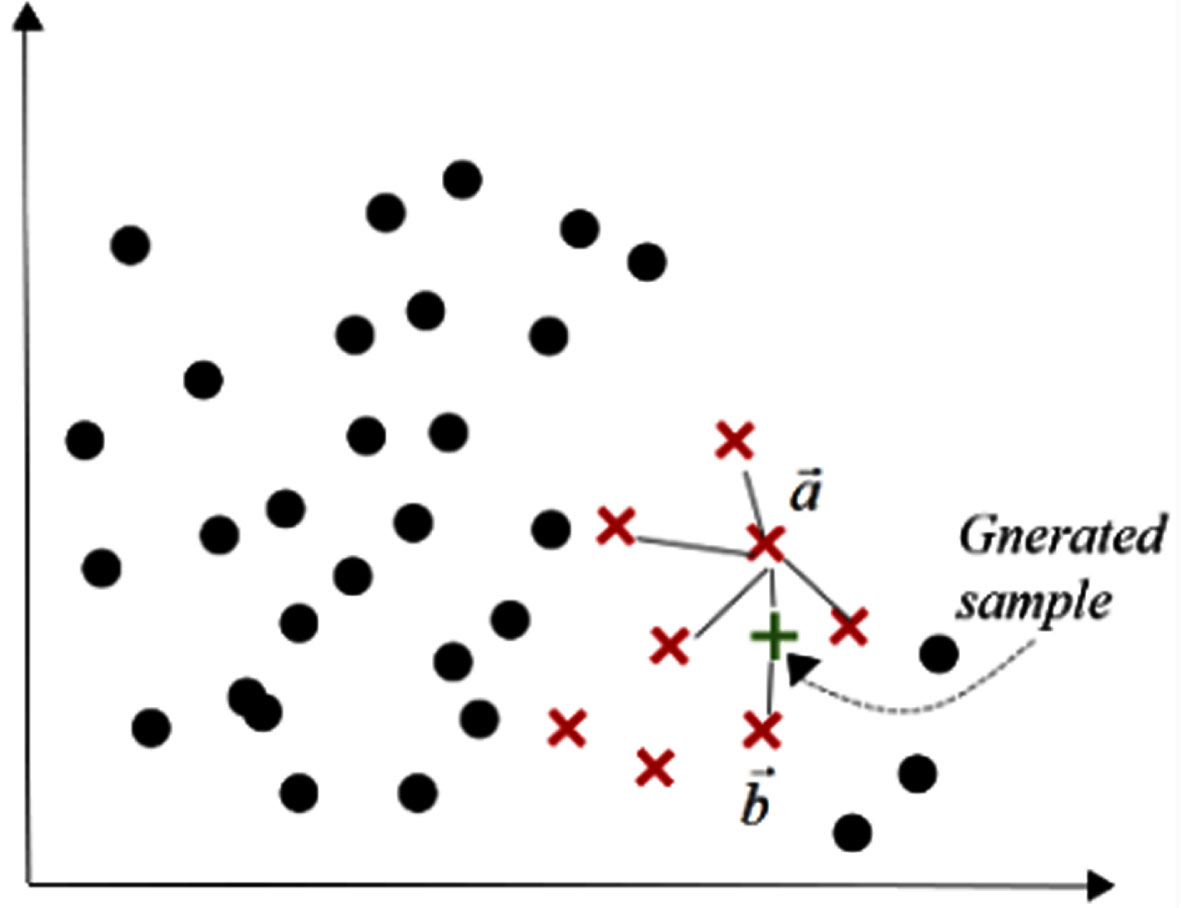
Randomly interpolate between the two samples by $\tilde{x} = \tilde{a} + ω \times (\tilde{b} - \tilde{a})$ , $\tilde{x}$ is a new generated sample. ω is a random weight in [0, 1].

Fig. 1

SMOTE randomly selected a minority sample for linear interpolation (k = 4).

However, as illustrated in Fig. 2, the algorithm has some weaknesses. One of them is that it does not address the within-class imbalance [14]. More samples are generated in areas with dense samples, while fewer samples are generated in areas with sparse samples. Another drawback is that SMOTE may further amplify the noise that exists in the data.

Fig. 2

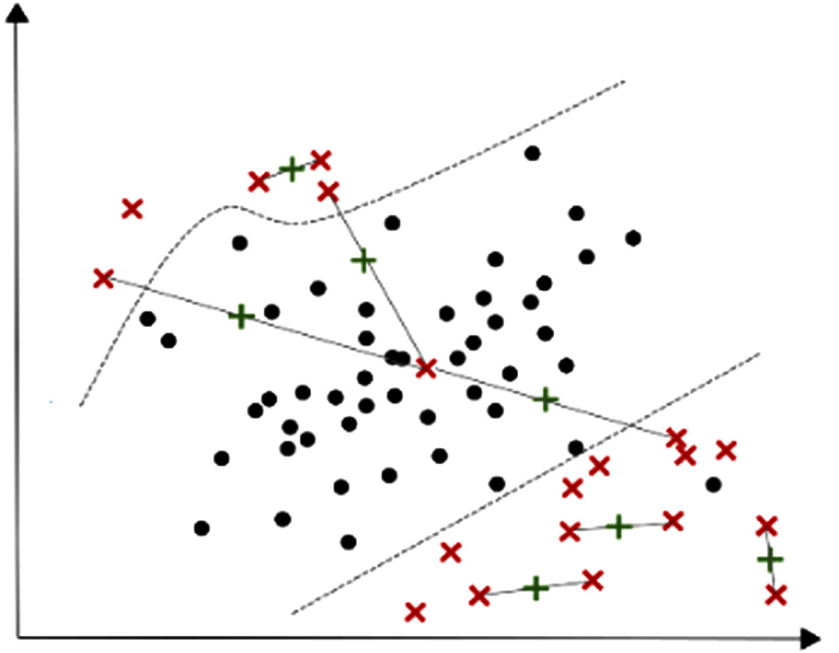
SMOTE may generate minority samples in majority regions (Noise samples). Most non-noise samples are generated in dense minority areas, contributing to within-class imbalance.

There are multiple variations of SMOTE which aim to combat the original algorithm’s weaknesses. Yet, many of these approaches are either very complex or alleviate only a few of SMOTE’s shortcomings. This work proposes combining the K-means clustering algorithm with SMOTE to address some of the drawbacks of previous oversampling algorithms with a simple-to-use technique [10].

2.2 K-means algorithm

K-means is a very important clustering algorithm in cluster analysis. The idea of the K-means algorithm is that, for a given sample set, the sample set is divided into K clusters according to the distance between the samples [23]. Let the points in the cluster be as close together as possible, and let the distance between the clusters be as wide as possible. The K-means can be summarized as:

For each training sample {x⁽¹⁾, … x⁽ⁱ⁾ }, x⁽ⁱ⁾ ∈ Rⁿ.

Randomly select cluster centroids points as μ₁, … μ_k, μ_i ∈ Rⁿ.

Assigning each sample i to the nearby cluster centroids. Formula is as follows: $c^{(i)} = arg min_{j} x^{(i)} - μ_{j}^{2}$ (1)

For each cluster j, use Equation (2) to recalculate the centroid of the class. $μ_{j} = \frac{\sum_{i = 1}^{m} 1 {c^{(i)} = j} x^{(i)}}{\sum_{i = 1}^{m} 1 {c^{(i)} = j}}$ (2)

Repeat steps until the centroid position is no longer updated and the algorithm converges [13]. The algorithm iteration process is shown in Fig. 3. All the parameters of K-means are also parameters of the algorithm in this paper, and the most significant one is the number of clusters K.

Fig. 3

The iterative process of K-means algorithm.

3 Proposed method

The proposed method ABWSMO adopts the popular K-means clustering algorithm, combined with SMOTE oversampling technology, and fuses the idea of boundary weighting to rebalance the dataset. It manages to avoid the generation of noise by oversampling only in safe areas [18]. At the same time, the sampling weight of the sample is determined by the number of majority samples in the k nearest neighbors of the minority boundary point. The regions closer to the boundary in minority samples are given higher sampling weights, so that the samples are generated closer to the boundary in preference. The classification performance of the classifier is improved by increasing the learning of the difficult-to-learn samples at the boundary, resolving the imbalance between and within classes.

3.1 Adaptive boundary weight adjustment strategy

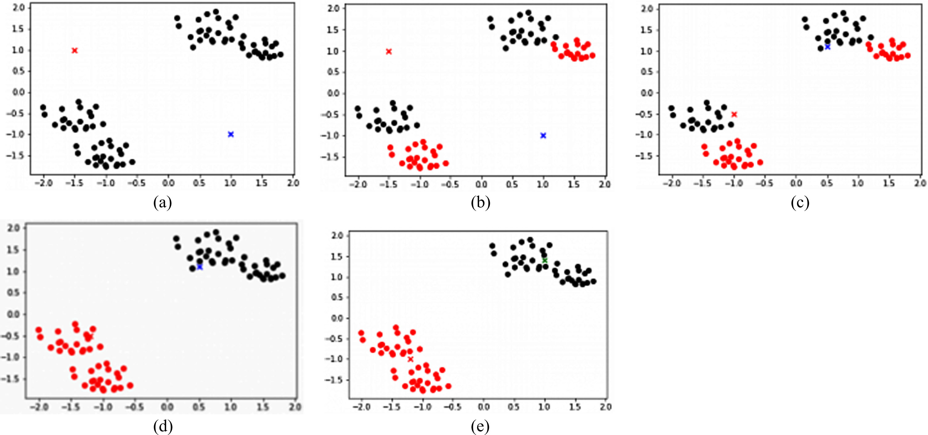
There are various techniques to quantify the importance and learning difficulty of a boundary sample based on the distance between minority and majority samples [9]. First, look for the center of the majority samples. The set of minority samples with the smallest distance within a certain threshold will represent the most informative and important boundary samples. As illustrated in Fig. 4(a), The ‘×’ in the figure represents minority samples, the ‘circle’ represents the majority samples, and the ‘diamond’ represents the center of the majority samples. Calculate the Euclidean distances between minority samples M₁, M₂, M₃, M₄, M₅ and the center of majority samples. As shown in Fig. 4(b), this method exhibits a critical flaw. If the majority class contains two clusters, each majority class must find its nearest cluster center before the minority sample calculates the distance to the center of the majority class, which increases the computational difficulty and reduces the efficiency of the algorithm. The adaptive boundary weight adjustment strategy of the ABWSMO algorithm does not look for the center of majority samples. The sampling weight is determined by the number of majority samples in the K nearest neighbors of each minority sample, and the value is taken as the local sample sampling weight. As illustrated in Fig. 4(c). The highlighted region surrounded by a dotted circle represents the K nearest neighbors search regions for minority samples M₁, M₂, M₃, M₄, M₅. Therefore, in the 4 nearest neighbors of M₁, M₂, M₃, M₄, M₅, accordingly, there are 3, 1, 2, 1, and 0 majority samples. This means that minority sample M₁ is more likely to be near the decision boundary. Therefore, more synthetic samples should be generated for M₁, assigning higher local boundary sample weights forces the classifier to pay more attention to the difficult-to-learn region of the boundary [11].

Fig .4

(a) A sample that determines the boundary based on Euclidean distance; (b) Shortcomings of the original method; (c) Use K nearest neighbors of each minority samples to calculate the weight.

Local sample weights can be calculated as follows:

In the sample of minority, for each minority sample M_i, its k_i nearest neighbors are found in the data set according to the Euclidean distance of n-dimensional space, which is defined as: $r_{i} = \frac{1}{1 + \exp (- α \cdot δ_{i})} i = 1, 2, \dots t$ (3)

(δ_i < k_i), Where δ_i is the number of majority samples in the k_i nearest neighbors. When δ_i = k_i, the sample is defined as noise sample. α is the proportionality coefficient, defined as 0.25 [22].

The larger r_i is, the more likely the sample is to be a boundary sample. Calculate the local sampling weight of each sample, Normalize r_i according to: ${\hat{r}}_{i} = \frac{r_{i}}{\sum_{i = 1}^{t} r_{i}}$ (4)

3.2 Adaptive over-sampling sample size determination strategy

One of the key issues in the oversampling algorithm is how to determine the global sampling weights. In other words, how many samples need to be generated per cluster [17]. In this paper, an adaptive oversampling sample size determination strategy is proposed to oversample only a few clusters with a relatively large proportion of minority samples. This method reduces the effect of noise. In addition, we aim to achieve within-class balance for minority samples. Therefore, the proposed oversampling strategy assigns more generated samples to sparse minority clusters than to dense ones. Whether or not each cluster is oversampled is determined by the proportion of minority and majority samples in the cluster. This can be adjusted by the imbalance rate threshold (or IR), a hyperparameter of ABWSMO which defaults to 1. The imbalance ratio of a cluster is defined as: $\frac{majcnt (a) + 1}{mincnt (a) + 1}$ .

A high sampling weight corresponds to minority samples with a low density and generates more samples. The calculation of global sampling weight can be expressed by four sub-calculations:

Randomly select cluster centroids points as μ₁, … μ_k, μ_i ∈ Rⁿ.

For each selected cluster, calculate the Euclidean distance matrix between the samples of the minority classes.

Calculate the average distance within each cluster, add all the off-diagonal elements of the distance matrix, and divide by the number of off-diagonal elements. To get the density of each cluster, the sample density is defined as: $DS (p) = \frac{\min cnt (p)}{average \min distance {(p)}^{f}}$ (5)

f is the number of features contained in the sample.

Sample sparsity is defined as: $SS (p) = \frac{1}{DS (p)}$ (6)

The global sampling weight of each cluster is defined as the sparsity of the cluster divided by the sum of the sparsities of all the clusters.

Therefore, the sum of all global sampling weights is 1. Because of this property, the global sampling weight of the cluster can be multiplied by the total number of samples to be generated, so as to determine the number of global samples to be generated in the cluster. After determining the global and local sampling weights of the samples, SMOTE algorithm is used to over-sample each selected cluster. For each cluster, for each minority sample, execute instruction ∥ samplingweight (p) × n ∥ × r_i to generate samples, where n is the total number of samples to be generated.

3.3 ABWSMO algorithm

The method proposed in this work uses the k-means clustering algorithm in combination with SMOTE oversampling. It avoids noise by oversampling only in safe regions. Furthermore, it focuses on between-class imbalances and within-class imbalances. What makes this method unique from related methods is not only its simplicity but also its novel and effective synthetic sample allocation strategy. Sample allocation is based on the density of clusters, producing more samples in sparse minority areas than in dense ones to eliminate within-class imbalance. Finally, overfitting is resisted by generating new samples rather than replicating them.

ABWSMO consists of four steps: marking minority boundary points and assigning local weights; clustering; selecting; and oversampling. The algorithm cleverly incorporates two innovative sample global and local weight determination strategies proposed in sections 3.1 and 3.2. An adaptive boundary weight adjustment strategy is used in the step of marking boundary points and assigning local weights. All majority and minority samples are input into the model, the boundary points are marked, and local sampling weights are assigned to each sample through the adaptive boundary weight adjustment strategy. In the clustering step, K-means clustering is used to cluster the input samples into K clusters.

The selection step selects the clustering for oversampling and retains the clustering with a high sample ratio of minority samples.

An oversampling sample size strategy is applied to assign global sample weights to each cluster, that is, the total number of samples to be generated for each cluster to be oversampled, and allocate more samples to minority clusters with sparse samples. Finally, in the over-sampling step, the SMOTE algorithm is applied to each minority sample in each selected cluster to achieve the target proportion of minority and majority samples. The sampling process of this algorithm is shown in Fig. 5.

Fig. 5

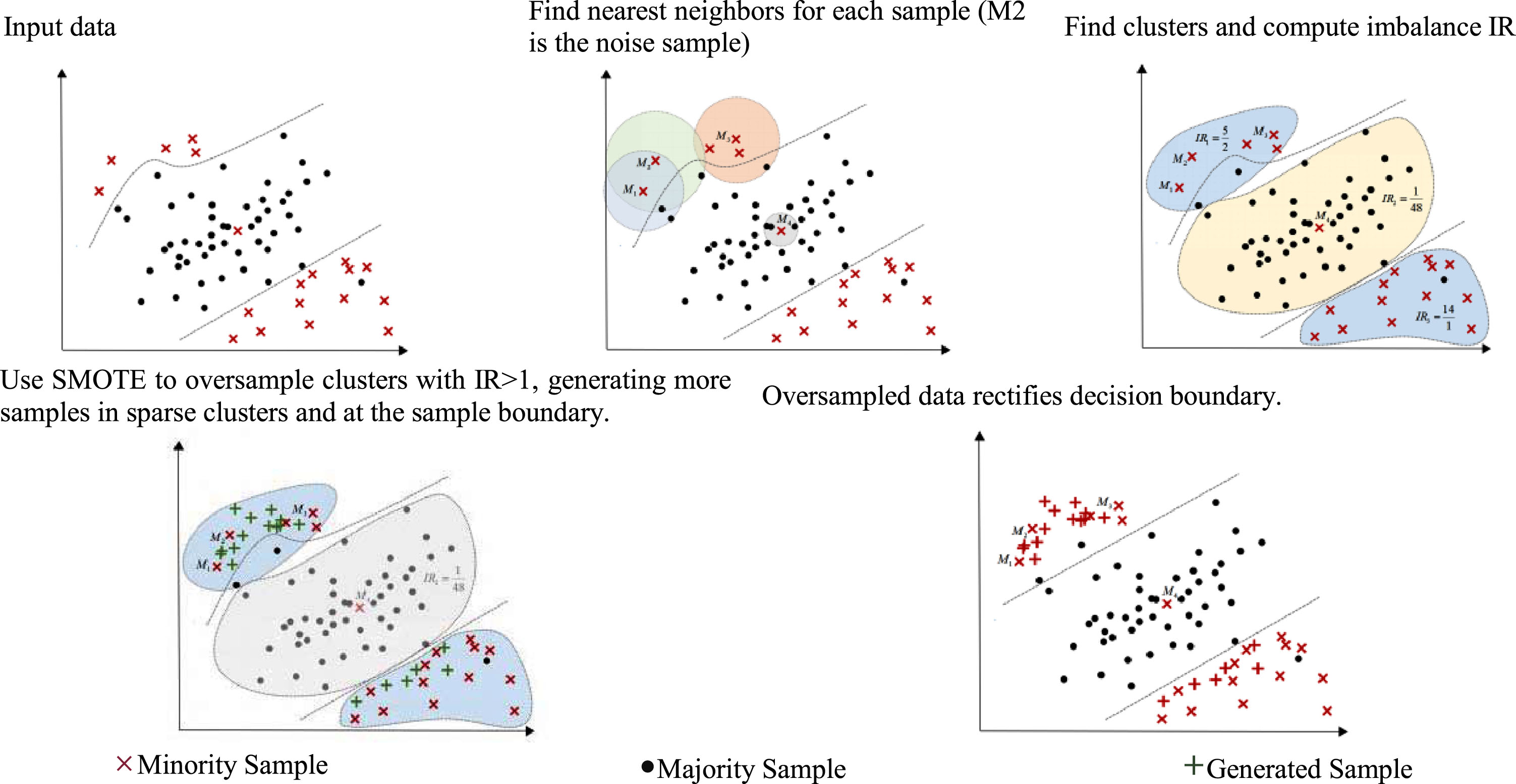
ABWSMO sampling procedure description.

This method is not only simple, but also a new and effective method for synthesizing sample distribution. The sample distribution is based on the clustering density, and more samples are generated in the sparse area of minority samples than in the dense area of minority samples, so as to overcome the within-class imbalance. By assigning a higher local sampling weight to minority class boundary points, the learning intensity of the classifier on boundary samples is increased. In addition, this method clusters without considering the category label so that safe over-sampling areas can be detected. Finally, overfitting is offset by generating minority samples rather than simply copying them.

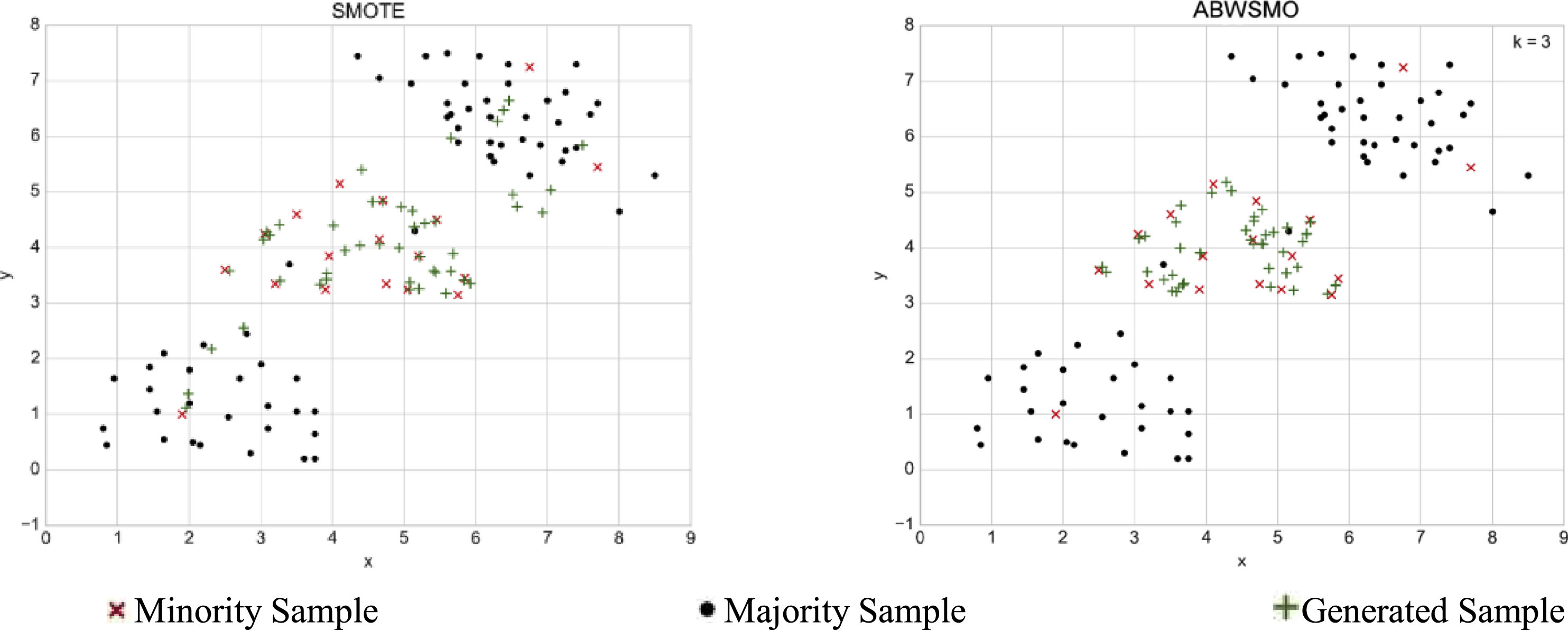
In order to illustrate the effectiveness of the ABWSMO oversampling algorithm, three two-dimensional arrays are used to illustrate. They are created for this work, consist of minority clusters, majority clusters, and noisy clusters. They are referred to as datasets A, B, and C. It can be clearly observed that the application of two innovative local and global sample determination strategies applied to the ABWSMO algorithm effectively avoids noise generation. In contrast to the traditional SMOTE algorithm, the ABWSMO algorithm prioritises the generation of samples near the boundary points. As shown in Figs. 6 –8, it is clear that oversampling via the ABWSMO algorithm effectively avoids the generation of noise compared to the traditional oversampling SMOTE algorithm, while generating samples preferentially close to the boundary points. The problem of imbalance within and between classes is solved, while the effect of class overlap on the oversampling algorithm is eliminated.

Fig. 6

Samples generated through oversampling dataset A with SMOTE and ABWSO.

Fig. 7

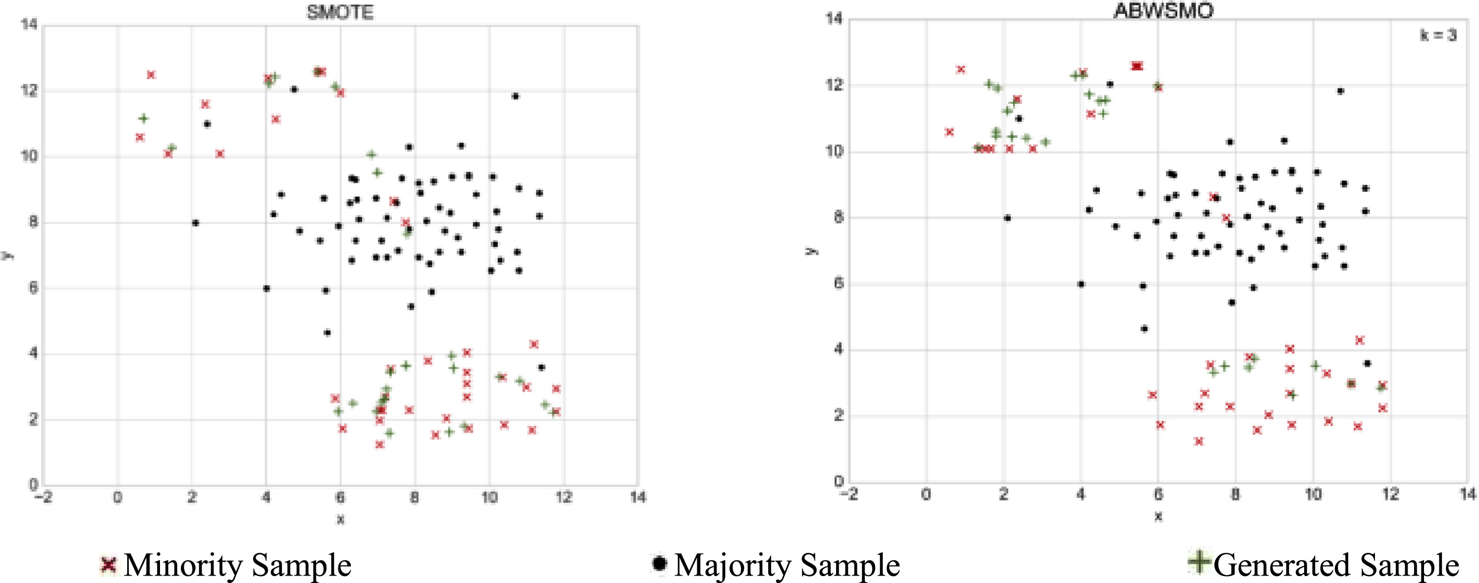
Samples generated through oversampling dataset B with SMOTE and ABWSO.

Fig. 8

Samples generated through oversampling dataset C with SMOTE and ABWSO.

4 Research methodology

4.1 Dataset description

The performance of ABWSMO is evaluated on 13 datasets from the UCI machine learning repository [4]. These datasets vary in size and class distributions to ensure a thorough assessment of performance. Table 1 summarizes the characteristics of the datasets used in our simulation. To ensure a full evaluation of performance, convert a dataset with two or more classes to a dataset with two classes for a majority class and a minority class. In addition, the Python library scikit-learn was used to generate three variations of the artificial “MADELON” dataset, which poses a difficult binary classification problem.

Table 1
Imbalance datasets

# Dataset Minority class Majority class # of features # of instances # of minority instances # of majority instances Imbalanced ratio

1 Vehicle Class “van” All other 17 846 199 647 1 : 3.25

2 Pima Class “pp” All other 7 336 52 259 1 : 4.98

3 Ecoli Class “2” All other 4 625 49 576 1 : 11.76

4 Liver disorders Class “1” All other 6 345 145 200 1 : 1.38

5 Wine Class “2” All other 13 178 71 130 1 : 1.83

6 Libra Class “1”, “2”, “3” All other 90 360 72 288 1 : 4.00

7 LEV Class “1” All other 4 1000 93 907 1 : 9.75

8 Iris Class “2” All other 4 150 50 100 1 : 2.00

9 Heart Class “1” Class”-1” 13 270 120 150 1 : 1.25

10 Glass Class “1” All other 9 214 70 138 1 : 1.97

11 Haberman Class “2” Class”1” 3 306 81 225 1 : 2.78

12 Segment Class of “WINDOW” All other 18 2310 330 1980 1 : 6.00

13 Breast tissue Class “Car”, “fad” All other 9 106 36 70 1 : 1.94

14 Simulated1 Class “min” Class “maj” 200 3000 15 2985 1 : 199.00

15 Simulated2 Class “min” Class “maj” 200 3000 13 2987 1 : 229.77

16 Simulated3 Class “min” Class “maj” 200 3000 22 2978 1 : 135.36

#	Dataset	Minority class	Majority class	# of features	# of instances	# of minority instances	# of majority instances	Imbalanced ratio
1	Vehicle	Class “van”	All other	17	846	199	647	1 : 3.25
2	Pima	Class “pp”	All other	7	336	52	259	1 : 4.98
3	Ecoli	Class “2”	All other	4	625	49	576	1 : 11.76
4	Liver disorders	Class “1”	All other	6	345	145	200	1 : 1.38
5	Wine	Class “2”	All other	13	178	71	130	1 : 1.83
6	Libra	Class “1”, “2”, “3”	All other	90	360	72	288	1 : 4.00
7	LEV	Class “1”	All other	4	1000	93	907	1 : 9.75
8	Iris	Class “2”	All other	4	150	50	100	1 : 2.00
9	Heart	Class “1”	Class”-1”	13	270	120	150	1 : 1.25
10	Glass	Class “1”	All other	9	214	70	138	1 : 1.97
11	Haberman	Class “2”	Class”1”	3	306	81	225	1 : 2.78
12	Segment	Class of “WINDOW”	All other	18	2310	330	1980	1 : 6.00
13	Breast tissue	Class “Car”, “fad”	All other	9	106	36	70	1 : 1.94
14	Simulated1	Class “min”	Class “maj”	200	3000	15	2985	1 : 199.00
15	Simulated2	Class “min”	Class “maj”	200	3000	13	2987	1 : 229.77
16	Simulated3	Class “min”	Class “maj”	200	3000	22	2978	1 : 135.36

4.2 Metrics

There are metrics which have been employed or developed specifically to cope with imbalanced data [25]. In this article, the performance measures used to compare the different approaches are: F-measure, G-mean, and Area under Receiving Operator Characteristic Graph (AUC). A confusion matrix (Table 2) can be constructed to illustrate the alignment of predictions with the true distribution. In the confusion matrix, minority instances are referred to as positive (P) and majority instances are referred to as negative (N).

Table 2
Confusion matrix

P N

Positives Negatives

PP TP FP

Predicted True False

Positives Positives Positives

PN FN TN

Predicted False True

Negatives Negatives Negatives

	P	N
PP	TP	FP
Predicted	True	False
Positives	Positives	Positives
PN	FN	TN
Predicted	False	True
Negatives	Negatives	Negatives

Precision measures the accuracy of the classifier, which means that a sample that is predicted to be positive is actually positive. Recall measures the completeness of the classifier, that is, the number of samples from minority categories that are correctly classified as positive. Parameter β of F_measure adjusts the relative importance between Precision and Recall. F_measure can be calculated by the following formula: $precision = \frac{TP}{TP + FP}$ (7) $recall = \frac{TP}{TP + FN}$ (8) $F_{measure} = \frac{(1 + β^{2}) * recall * precision}{β^{2} * recall + precision}$ (9)G_mean considers the accuracy for both classes. The higher G_mean can be obtained only when the accuracy of both classes is high. G_mean is determined as follows: $G_{mean} = \sqrt{\frac{TP}{TP + FN} \times \frac{TN}{TN + FP}}$ (10) Another effective method to evaluate the performance of imbalanced data classification is the AUC (Area Under the ROC Curve). The ROC curve has been widely used as a visualization technology for classifier evaluation. The closer the ROC curve is to the upper left, the stronger the discrimination ability of the corresponding classifier is. AUC can quantitatively represent the classifier performance corresponding to the ROC curve. The ROC defined as follows: $ROC = \frac{TRP}{FRP} = \frac{TP}{N} \cdot \frac{N_{n}}{FP}$ (11)

4.3 Experiments

The ultimate goal of any oversampling method is to improve the classification results. In other words, an oversampling algorithm is successful if the oversampled data it produces improves the predictive quality and classification performance of a given classifier. In this paper, the proposed ABWSMO method is evaluated on 13 datasets from the UCI database and compared with the other 5 oversampling methods: Random-OverSampling; SMOTE; Boderline1-SMOTE; Boderline2-SMOTE; Cluster-SMOTE.

In order to determine the mean and standard deviation of the performance measures for the over-sampling methods, 4-fold cross validation was used. Each experiment was repeated 3 times report the average in order to alleviate the randomness effects on the results. The criteria for cross validation are G_mean, because it explains all the value indicators in the confusion matrix and provides a more reliable measure for learning from unbalanced data.

In order to evaluate the various oversampling methods, several different classifiers were chosen to ensure that the results obtained could be generalized and not limited by the use of a particular classifier. The choice of classifier was also influenced by the number of hyperparameters: classification algorithms with few or no hyperparameters were preferred. Classification algorithms with few or no hyperparameters are less likely to bias the results due to their specific configuration. With reference to the experience of previous research by experts and scholars, the following classifiers are chosen for this paper. SVM is a common binary classification algorithm that is highly representative for classifying small data sets. For the SVM classifier, the parameter is selected from the values (2^-1, 2⁰, 2¹). For KNN, select the nearest neighbor among the values (4, 5, 6). LR does not need to adjust any parameters [20].

4.4 Results discussions

Tables 3 –5 shows the results of the mean and standard deviation of our proposed ABWSMO method and the other 5 sampling methods using these 3 classifiers on 16 datasets. The best classification algorithm is shown in bold. ABWSMO obtains the best results according to at least one of the measures in 14 out of the 16 datasets when KNN was used and in 15 out of the 16 datasets when SVM and LR were used. For example, in Table 3, on the dataset “Vehicle”, ABWSMO performs best in all three metrics compared to the other five classification algorithms, reaching 0.937, 0.964, and 0.992. Of the six algorithms tested on the dataset “Pima”, Cluster SMOTE performed best in two evaluation metrics, while ABWSMO performed best in one evaluation metric.

Table 3
Results for the Sampling methods on the 13 datasets classified using KNN

Dataset Meas Random oversampling SMOTE Borderline1 SMOTE Borderline2 SMOTE Cluster SMOTE ABWSMO

Vehicle F_M 0.921±0.013 0.953±0.019 0.922±.014 0.934±0.004 0.926±0.022 0.937±0.003

G_M 0.963±0.007 0.963±0.005 0.950±0.010 0.962±0.011 0.963±0.003 0.964±0.005

AUC 0.971±0.011 0.990±0.003 0.962±0.006 0.986±0.012 0.991±0.006 0.992±0.021

Pima F_M 0.591±0.047 0.589±0.080 0.596±0.014 0.607±0.062 0.660±0.037 0.642±0.017

G_M 0.683±0.060 0.678±0.019 0.687±0.071 0.693±0.031 0.736±0.031 0.732±0.012

AUC 0.767±0.080 0.757±0.069 0.714±0.063 0.767±0.056 0.822±0.036 0.833±0.002

Ecoli F_M 0.844±0.005 0.863±0.023 0.756±0.069 0.832±0.067 0.671±0.230 0.887±0.032

G_M 0.933±0.039 0.940±0.021 0.905±0.021 0.923±0.030 0.853±0.024 0.942±0.012

AUC 0.954±0.030 0.957±0.028 0.947±0.028 0.953±0.034 0.949±0.003 0.953±0.033

Liver F_M 0.592±0.023 0.576±0.039 0.596±0.031 0.547±0.039 0.581±0.037 0.563±0.064

G_M 0.561±0.025 0.554±0.044 0.569±0.019 0.554±0.023 0.550±0.040 0.567±0.031

AUC 0.608±0.044 0.602±0.035 0.629±0.044 0.617±0.021 0.611±0.037 0.627±0.030

Wine F_M 0.950±0.030 0.953±0.023 0.958±0.032 0.954±0.011 0.956±0.024 0.979±0.020

G_M 0.956±0.023 0.960±0.013 0.965±0.023 0.953±0.025 0.964±0.022 0.973±0.019

AUC 0.990±0.010 0.990±0.012 0.992±0.012 0.968±0.033 0.990±0.014 0.991±0.013

Libra F_M 0.973±0.013 0.979±0.011 0.946±0.025 0.974±0.023 0.949±0.039 0.983±0.020

G_M 0.983±0.014 0.983±0.015 0.969±0.024 0.968±0.012 0.978±0.022 0.985±0.018

AUC 0.985±0.015 0.988±0.015 0.974±0.023 0.977±0.028 0.992±0.012 0.987±0.011

LEV F_M 0.446±0.033 0.451±0.022 0.436±0.038 0.469±0.056 0.474±0.072 0.473±0.066

G_M 0.761±0.023 0.755±0.034 0.759±0.032 0.668±0.038 0.755±0.045 0.649±0.051

AUC 0.795±0.034 0.799±0.042 0.787±0.037 0.790±0.050 0.814±0.060 0.782±0.043

Iris F_M 0.937±0.032 0.952±0.030 0.916±0.042 0.925±0.032 0.937±0.039 0.953±0.013

G_M 0.956±0.022 0.972±0.016 0.946±0.030 0.955±0.020 0.959±0.029 0.976±0.032

AUC 0.975±0.043 0.985±0.012 0.973±0.026 0.972±0.024 0.979±0.020 0.983±0.023

Heart F_M 0.849±0.024 0.816±0.031 0.809±0.014 0.835±0.033 0.823±0.027 0.853±0.021

G_M 0.857±0.021 0.828±0.029 0.812±0.013 0.845±0.021 0.835±0.023 0.862±0.018

AUC 0.988±0.023 0.880±0.030 0.876±0.015 0.891±0.015 0.894±0.019 0.913±0.021

Glass F_M 0.708±0.023 0.727±0.021 0.696±0.034 0.674±0.021 0.702±0.031 0.732±0.023

G_M 0.856±0.021 0.803±0.017 0.773±0.024 0.754±0.032 0.778±0.027 0.808±0.011

AUC 0.903±0.010 0.855±0.019 0.844±0.048 0.830±0.020 0.853±0.026 0.861±0.022

Haberman F_M 0.441±0.023 0.393±0.068 0.403±0.071 0.385±0.039 0.447±0.043 0.383±0.023

G_M 0.590±0.018 0.552±0.062 0.559±0.068 0.563±0.033 0.593±0.042 0.548±0.024

AUC 0.594±0.015 0.566±0.054 0.324±0.018 0.586±0.029 0.609±0.042 0.587±0.011

Segment F_M 0.833±0.027 0.837±0.023 0.829±0.019 0.838±0.015 0.833±0.041 0.844±0.031

G_M 0.947±0.011 0.956±0.010 0.945±0.032 0.954±0.026 0.953±0.013 0.936±0.016

AUC 0.966±0.011 0.973±0.012 0.973±0.011 0.981±0.010 0.978±0.003 0.953±0.023

Heating F_M 0.697±0.011 0.711±0.030 0.707±0.044 0.733±0.013 0.716±0.021 0.744±0.042

G_M 0.821±0.022 0.835±0.021 0.834±0.035 0.854±0.015 0.841±0.015 0.852±0.012

AUC 0.874±0.014 0.875±0.016 0.866±0.023 0.878±0.024 0.897±0.013 0.874±0.023

Simulated1 F_M 0.541±0.010 0.652±0.009 0.728±0.039 0.715±0.013 0.716±0.021 0.737±0.038

G_M 0.687±0.027 0.795±0.012 0.811±0.025 0.837±0.014 0.841±0.015 0.830±0.022

AUC 0.662±0.033 0.835±0.011 0.850±0.019 0.876±0.024 0.897±0.013 0.878±0.023

Simulated2 F_M 0.552±0.018 0.702±0.041 0.712±0.044 0.721±0.015 0.693±0.025 0.790±0.031

G_M 0.711±0.030 0.725±0.032 0.814±0.027 0.841±0.019 0.743±0.018 0.840±0.012

AUC 0.694±0.016 0.861±0.015 0.852±0.019 0.862±0.024 0.857±0.013 0.864±0.023

Simulated3 F_M 0.632±0.021 0.671±0.023 0.697±0.023 0.711±0.024 0.732±0.023 0.745±0.044

G_M 0.705±0.015 0.821±0.015 0.825±0.018 0.832±0.013 0.867±0.013 0.861±0.022

AUC 0.812±0.015 0.825±0.026 0.836±0.016 0.862±0.022 0.895±0.013 0.875±0.023

Dataset	Meas	Random oversampling	SMOTE	Borderline1 SMOTE	Borderline2 SMOTE	Cluster SMOTE	ABWSMO
Vehicle	F_M	0.921±0.013	0.953±0.019	0.922±.014	0.934±0.004	0.926±0.022	0.937±0.003
	G_M	0.963±0.007	0.963±0.005	0.950±0.010	0.962±0.011	0.963±0.003	0.964±0.005
	AUC	0.971±0.011	0.990±0.003	0.962±0.006	0.986±0.012	0.991±0.006	0.992±0.021
Pima	F_M	0.591±0.047	0.589±0.080	0.596±0.014	0.607±0.062	0.660±0.037	0.642±0.017
	G_M	0.683±0.060	0.678±0.019	0.687±0.071	0.693±0.031	0.736±0.031	0.732±0.012
	AUC	0.767±0.080	0.757±0.069	0.714±0.063	0.767±0.056	0.822±0.036	0.833±0.002
Ecoli	F_M	0.844±0.005	0.863±0.023	0.756±0.069	0.832±0.067	0.671±0.230	0.887±0.032
	G_M	0.933±0.039	0.940±0.021	0.905±0.021	0.923±0.030	0.853±0.024	0.942±0.012
	AUC	0.954±0.030	0.957±0.028	0.947±0.028	0.953±0.034	0.949±0.003	0.953±0.033
Liver	F_M	0.592±0.023	0.576±0.039	0.596±0.031	0.547±0.039	0.581±0.037	0.563±0.064
	G_M	0.561±0.025	0.554±0.044	0.569±0.019	0.554±0.023	0.550±0.040	0.567±0.031
	AUC	0.608±0.044	0.602±0.035	0.629±0.044	0.617±0.021	0.611±0.037	0.627±0.030
Wine	F_M	0.950±0.030	0.953±0.023	0.958±0.032	0.954±0.011	0.956±0.024	0.979±0.020
	G_M	0.956±0.023	0.960±0.013	0.965±0.023	0.953±0.025	0.964±0.022	0.973±0.019
	AUC	0.990±0.010	0.990±0.012	0.992±0.012	0.968±0.033	0.990±0.014	0.991±0.013
Libra	F_M	0.973±0.013	0.979±0.011	0.946±0.025	0.974±0.023	0.949±0.039	0.983±0.020
	G_M	0.983±0.014	0.983±0.015	0.969±0.024	0.968±0.012	0.978±0.022	0.985±0.018
	AUC	0.985±0.015	0.988±0.015	0.974±0.023	0.977±0.028	0.992±0.012	0.987±0.011
LEV	F_M	0.446±0.033	0.451±0.022	0.436±0.038	0.469±0.056	0.474±0.072	0.473±0.066
	G_M	0.761±0.023	0.755±0.034	0.759±0.032	0.668±0.038	0.755±0.045	0.649±0.051
	AUC	0.795±0.034	0.799±0.042	0.787±0.037	0.790±0.050	0.814±0.060	0.782±0.043
Iris	F_M	0.937±0.032	0.952±0.030	0.916±0.042	0.925±0.032	0.937±0.039	0.953±0.013
	G_M	0.956±0.022	0.972±0.016	0.946±0.030	0.955±0.020	0.959±0.029	0.976±0.032
	AUC	0.975±0.043	0.985±0.012	0.973±0.026	0.972±0.024	0.979±0.020	0.983±0.023
Heart	F_M	0.849±0.024	0.816±0.031	0.809±0.014	0.835±0.033	0.823±0.027	0.853±0.021
	G_M	0.857±0.021	0.828±0.029	0.812±0.013	0.845±0.021	0.835±0.023	0.862±0.018
	AUC	0.988±0.023	0.880±0.030	0.876±0.015	0.891±0.015	0.894±0.019	0.913±0.021
Glass	F_M	0.708±0.023	0.727±0.021	0.696±0.034	0.674±0.021	0.702±0.031	0.732±0.023
	G_M	0.856±0.021	0.803±0.017	0.773±0.024	0.754±0.032	0.778±0.027	0.808±0.011
	AUC	0.903±0.010	0.855±0.019	0.844±0.048	0.830±0.020	0.853±0.026	0.861±0.022
Haberman	F_M	0.441±0.023	0.393±0.068	0.403±0.071	0.385±0.039	0.447±0.043	0.383±0.023
	G_M	0.590±0.018	0.552±0.062	0.559±0.068	0.563±0.033	0.593±0.042	0.548±0.024
	AUC	0.594±0.015	0.566±0.054	0.324±0.018	0.586±0.029	0.609±0.042	0.587±0.011
Segment	F_M	0.833±0.027	0.837±0.023	0.829±0.019	0.838±0.015	0.833±0.041	0.844±0.031
	G_M	0.947±0.011	0.956±0.010	0.945±0.032	0.954±0.026	0.953±0.013	0.936±0.016
	AUC	0.966±0.011	0.973±0.012	0.973±0.011	0.981±0.010	0.978±0.003	0.953±0.023
Heating	F_M	0.697±0.011	0.711±0.030	0.707±0.044	0.733±0.013	0.716±0.021	0.744±0.042
	G_M	0.821±0.022	0.835±0.021	0.834±0.035	0.854±0.015	0.841±0.015	0.852±0.012
	AUC	0.874±0.014	0.875±0.016	0.866±0.023	0.878±0.024	0.897±0.013	0.874±0.023
Simulated1	F_M	0.541±0.010	0.652±0.009	0.728±0.039	0.715±0.013	0.716±0.021	0.737±0.038
	G_M	0.687±0.027	0.795±0.012	0.811±0.025	0.837±0.014	0.841±0.015	0.830±0.022
	AUC	0.662±0.033	0.835±0.011	0.850±0.019	0.876±0.024	0.897±0.013	0.878±0.023
Simulated2	F_M	0.552±0.018	0.702±0.041	0.712±0.044	0.721±0.015	0.693±0.025	0.790±0.031
	G_M	0.711±0.030	0.725±0.032	0.814±0.027	0.841±0.019	0.743±0.018	0.840±0.012
	AUC	0.694±0.016	0.861±0.015	0.852±0.019	0.862±0.024	0.857±0.013	0.864±0.023
Simulated3	F_M	0.632±0.021	0.671±0.023	0.697±0.023	0.711±0.024	0.732±0.023	0.745±0.044
	G_M	0.705±0.015	0.821±0.015	0.825±0.018	0.832±0.013	0.867±0.013	0.861±0.022
	AUC	0.812±0.015	0.825±0.026	0.836±0.016	0.862±0.022	0.895±0.013	0.875±0.023

Table 4

Results for the Sampling methods on the 13 datasets classified using SVM

Dataset	Meas	Random oversampling	SMOTE	Borderline1 SMOTE	Borderline2 SMOTE	Cluster SMOTE	ABWSMO
Vehicle	F_M	0.944±0.023	0.953±0.019	0.947±0.013	0.934±0.004	0.858±0.099	0.952±0.021
	G_M	0.958±0.018	0.969±0.013	0.961±0.015	0.960±0.011	0.931±0.064	0.971±0.016
	AUC	0.984±0.011	0.993±0.005	0.985±0.006	0.984±0.012	0.989±0.013	0.984±0.012
Pima	F_M	0.584±0.078	0.589±0.080	0.586±0.076	0.625±0.044	0.660±0.037	0.676±0.023
	G_M	0.673±0.080	0.678±0.019	0.672±0.071	0.674±0.031	0.736±0.031	0.752±0.020
	AUC	0.788±0.083	0.757±0.069	0.745±0.063	0.748±0.036	0.822±0.036	0.843±0.022
Ecoli	F_M	0.844±0.005	0.863±0.023	0.756±0.069	0.832±0.067	0.671±0.230	0.887±0.032
	G_M	0.933±0.039	0.940±0.021	0.905±0.021	0.923±0.030	0.853±0.024	0.942±0.012
	AUC	0.954±0.030	0.957±0.028	0.947±0.028	0.953±0.034	0.949±0.003	0.953±0.033
Liver	F_M	0.623±0.023	0.607±0.055	0.617±0.043	0.646±0.045	0.582±0.030	0.603±0.022
	G_M	0.668±0.025	0.655±0.040	0.669±0.023	0.692±0.012	0.535±0.012	0.649±0.021
	AUC	0.726±0.024	0.727±0.035	0.724±0.034	0.744±0.022	0.661±0.035	0.718±0.030
Wine	F_M	0.966±0.010	0.976±0.020	0.976±0.020	0.976±0.022	0.973±0.023	0.979±0.020
	G_M	0.959±0.011	0.978±0.018	0.978±0.018	0.978±0.012	0.979±0.012	0.979±0.017
	AUC	0.997±0.001	0.999±0.001	0.999±0.001	0.999±0.001	0.999±0.001	0.999±0.001
Libra	F_M	0.508±0.085	0.615±0.140	0.552±0.071	0.610±0.092	0.803±0.033	0.692±0.046
	G_M	0.724±0.072	0.746±0.115	0.762±0.068	0.750±0.082	0.828±0.042	0.721±0.046
	AUC	0.994±0.007	0.993±0.007	0.994±0.013	0.994±0.007	0.988±0.012	0.994±0.018
LEV	F_M	0.478±0.048	0.510±0.0453	0.460±0.049	0.566±0.046	0.452±0.072	0.557±0.028
	G_M	0.736±0.056	0.746±0.049	0.735±0.043	0.760±0.043	0.763±0.045	0.799±0.051
	AUC	0.737±0.044	0.750±0.053	0.756±0.057	0.783±0.060	0.834±0.060	0.863±0.046
Iris	F_M	0.947±0.032	0.956±0.023	0.926±0.032	0.945±0.036	0.828±0.036	0.947±0.023
	G_M	0.964±0.012	0.972±0.016	0.950±0.031	0.961±0.029	0.961±0.029	0.961±0.19
	AUC	0.992±0.003	0.994±0.004	0.974±0.016	0.982±0.019	0.982±0.019	0.994±0.003
Heart	F_M	0.797±0.024	0.795±0.026	0.783±0.022	0.781±0.018	0.812±0.027	0.810±0.034
	G_M	0.817±0.020	0.815±0.017	0.802±0.014	0.802±0.033	0.828±0.023	0.829±0.040
	AUC	0.875±0.026	0.858±0.020	0.847±0.020	0.853±0.027	0.870±0.031	0.877±0.011
Glass	F_M	0.755±0.028	0.731±0.031	0.745±0.038	0.746±0.031	0.622±0.042	0.756±0.013
	G_M	0.828±0.028	0.804±0.041	0.818±0.043	0.821±0.030	0.709±0.067	0.831±0.011
	AUC	0.873±0.020	0.864±0.023	0.866±0.032	0.881±0.027	0.856±0.036	0.871±0.022
Haberman	F_M	0.445±0.036	0.420±0.044	0.446±0.061	0.412±0.035	0.399±0.051	0.428±0.050
	G_M	0.601±0.021	0.580±0.032	0.605±0.049	0.577±0.020	0.558±0.032	0.578±0.034
	AUC	0.661±0.031	0.653±0.041	0.637±0.045	0.643±0.024	0.641±0.039	0.667±0.033
Segment	F_M	0.863±0.016	0.886±0.031	0.844±0.016	0.876±0.012	0.696±0.058	0.887±0.003
	G_M	0.945±0.012	0.956±0.010	0.932±0.021	0.948±0.011	0.915±0.022	0.958±0.014
	AUC	0.979±0.007	0.983±0.003	0.978±0.006	0.972±0.002	0.976±0.006	0.982±0.015
Heating	F_M	NaN	0.591±0.021	0.583±0.021	0.733±0.013	0.696±0.031	0.748±0.042
	G_M	0.431±0.022	0.690±0.008	0.685±0.011	0.854±0.015	0.833±0.014	0.856±0.037
	AUC	0.854±0.017	0.875±0.016	0.864±0.013	0.878±0.024	0.889±0.047	0.910±0.021
Simulated1	F_M	0.637±0.036	0.641±0.013	0.728±0.031	0.715±0.013	0.724±0.022	0.733±0.032
	G_M	0.662±0.028	0.746±0.014	0.828±0.020	0.828±0.015	0.824±0.015	0.829±0.022
	AUC	0.685±0.023	0.841±0.020	0.845±0.021	0.862±0.020	0.877±0.013	0.877±0.023
Simulated2	F_M	0.651±0.017	0.713±0.035	0.734±0.031	0.753±0.023	0.674±0.015	0.789±0.024
	G_M	0.704±0.021	0.724±0.024	0.806±0.018	0.839±0.027	0.755±0.016	0.842±0.013
	AUC	0.689±0.014	0.845±0.016	0.848±0.025	0.853±0.018	0.843±0.012	0.841±0.020
Simulated3	F_M	0.664±0.022	0.658±0.025	0.682±0.022	0.723±0.023	0.737±0.007	0.755±0.032
	G_M	0.732±0.014	0.823±0.018	0.824±0.013	0.844±0.014	0.854±0.018	0.843±0.021
	AUC	0.806±0.016	0.831±0.016	0.855±0.017	0.856±0.013	0.843±0.015	0.866±0.024

Table 5

Results for the Sampling methods on the 13 datasets classified using LR

Dataset	Meas	Random oversampling	SMOTE	Borderline1 SMOTE	Borderline2 SMOTE	Cluster SMOTE	ABWSMO
Vehicle	F_M	0.932±0.020	0.934±0.020	0.924±0.014	0.941±0.014	0.931±0.030	0.924±0.023
	G_M	0.964±0.011	0.961±0.011	0.952±0.021	0.959±0.019	0.962±0.022	0.955±0.015
	AUC	0.991±0.006	0.991±0.003	0.986±0.006	0.990±0.008	0.992±0.021	0.993±0.006
Pima	F_M	0.589±0.071	0.588±0.072	0.586±0.076	0.612±0.062	0.659±0.037	0.660±0.016
	G_M	0.677±0.066	0.676±0.021	0.667±0.070	0.693±0.031	0.741±0.035	0.745±0.017
	AUC	0.758±0.074	0.755±0.059	0.744±0.063	0.768±0.062	0.842±0.031	0.853±0.023
Ecoli	F_M	0.723±0.031	0.696±0.034	0.623±0.043	0.701±0.027	0.693±0.025	0.728±0.022
	G_M	0.867±0.022	0.871±0.029	0.848±0.019	0.846±0.035	0.864±0.014	0.867±0.015
	AUC	0.923±0.016	0.935±0.028	0.914±0.026	0.923±0.018	0.928±0.023	0.934±0.034
Liver	F_M	0.606±0.053	0.628±0.041	0.624±0.061	0.636±0.033	0.617±0.035	0.646±0.024
	G_M	0.641±0.035	0.659±0.037	0.642±0.055	0.672±0.021	0.650±0.032	0.682±0.018
	AUC	0.714±0.032	0.709±0.026	0.719±0.023	0.731±0.030	0.728±0.025	0.718±0.031
Wine	F_M	0.956±0.024	0.945±0.031	0.946±0.027	0.941±0.011	0.945±0.030	0.953±0.030
	G_M	0.948±0.031	0.951±0.028	0.955±0.031	0.938±0.025	0.952±0.032	0.962±0.021
	AUC	0.994±0.004	0.995±0.006	0.994±0.0	0.995±0.003	0.995±0.002	0.997±0.002
Libra	F_M	0.486±0.101	0.513±0.099	0.502±0.083	0.521±0.090	0.499±0.109	0.543±0.089
	G_M	0.642±0.090	0.659±0.076	0.648±0.072	0.660±0.082	0.654±0.101	0.669±0.082
	AUC	0.708±0.092	0.707±0.103	0.701±0.088	0.703±0.098	0.703±0.101	0.707±0.092
LEV	F_M	0.438±0.021	0.463±0.022	0.390±0.034	0.571±0.054	0.448±0.045	0.590±0.071
	G_M	0.802±0.030	0.811±0.031	0.791±0.032	0.821±0.051	0.821±0.041	0.820±0.061
	AUC	0.887±0.031	0.890±0.029	0.886±0.031	0.892±0.030	0.892±0.033	0.899±0.030
Iris	F_M	0.936±0.021	0.929±0.031	0.942±0.017	0.943±0.013	0.941±0.019	0.944±0.012
	G_M	0.955±0.020	0.948±0.025	0.962±0.010	0.961±0.011	0.957±0.017	0.962±0.011
	AUC	0.990±0.007	0.991±0.007	0.990±0.008	0.992±0.006	0.993±0.005	0.995±0.002
Heart	F_M	0.861±0.021	0.847±0.028	0.847±0.031	0.843±0.030	0.853±0.027	0.853±0.021
	G_M	0.875±0.019	0.856±0.029	0.853±0.035	0.866±0.023	0.866±0.026	0.874±0.024
	AUC	0.930±0.011	0.931±0.015	0.926±0.021	0.927±0.013	0.932±0.015	0.929±0.011
Glass	F_M	0.638±0.032	0.637±0.041	0.627±0.043	0.632±0.049	0.640±0.051	0.661±0.023
	G_M	0.724±0.028	0.723±0.033	0.708±0.034	0.723±0.040	0.727±0.049	0.742±0.011
	AUC	0.831±0.032	0.835±0.026	0.816±0.034	0.828±0.035	0.824±0.036	0.839±0.022
Haberman	F_M	0.486±0.048	0.471±0.032	0.458±0.051	0.466±0.022	0.458±0.036	0.509±0.045
	G_M	0.634±0.040	0.616±0.033	0.611±0.044	0.626±0.027	0.606±0.044	0.648±0.051
	AUC	0.672±0.044	0.646±0.026	0.650±0.031	0.655±0.033	0.645±0.041	0.699±0.050
Segment	F_M	0.642±0.038	0.646±0.029	0.604±0.022	0.638±0.015	0.667±0.008	0.665±0.031
	G_M	0.878±0.012	0.879±0.017	0.852±0.034	0.854±0.026	0.873±0.005	0.876±0.016
	AUC	0.942±0.005	0.943±0.008	0.908±0.020	0.918±0.010	0.945±0.003	0.944±0.023
Heating	F_M	0.720±0.039	0.725±0.044	0.720±0.044	0.730±0.050	0.732±0.035	0.730±0.047
	G_M	0.839±0.038	0.844±0.026	0.843±0.035	0.841±0.033	0.839±0.026	0.845±0.044
	AUC	0.916±0.027	0.919±0.028	0.906±0.023	0.916±0.024	0.919±0.024	0.924±0.021
Simulated1	F_M	0.628±0.026	0.663±0.022	0.719±0.028	0.744±0.016	0.733±0.012	0.746±0.030
	G_M	0.654±0.017	0.735±0.016	0.818±0.024	0.819±0.018	0.835±0.015	0.811±0.024
	AUC	0.679±0.020	0.839±0.018	0.836±0.020	0.868±0.021	0.877±0.013	0.879±0.022
Simulated2	F_M	0.654±0.022	0.713±0.035	0.734±0.026	0.749±0.019	0.663±0.022	0.788±0.021
	G_M	0.781±0.019	0.724±0.024	0.825±0.013	0.841±0.028	0.769±0.015	0.843±0.013
	AUC	0.639±0.022	0.836±0.016	0.844±0.014	0.860±0.011	0.842±0.016	0.839±0.020
Simulated3	F_M	0.655±0.017	0.647±0.018	0.673±0.025	0.722±0.020	0.724±0.006	0.745±0.018
	G_M	0.726±0.015	0.816±0.022	0.829±0.023	0.831±0.015	0.848±0.012	0.841±0.024
	AUC	0.815±0.011	0.831±0.016	0.846±0.025	0.849±0.017	0.839±0.025	0.870±0.014

According to DEM’s [8] recommendations for evaluating classifier performance across multiple datasets, the resulting metrics are not compared simply, but rather sorted to produce a ranking. Figure 9 shows the average ranking of each method in terms of F-measure, G-mean, and AUC of all test data sets, with the best performing method ranking at 1 and the worst method ranking at 6. It can be seen that the ranking of ABWSMO is the best under the three evaluation indexes of the three classifiers, while the ranking of other oversampling algorithms is unstable. Combined with the Friedman test [12] and Holm’s method [27] this evaluation method is also used by other authors working on the topic of imbalanced classification.

Fig. 9

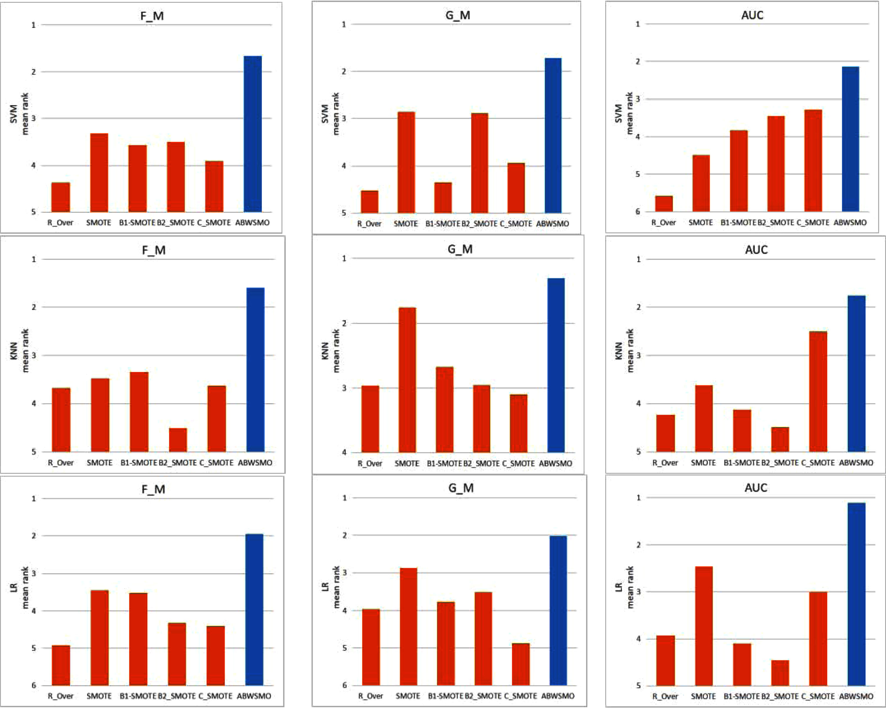
The mean ranking results of the 6 methods on 16 datasets (Best: 1; Worst: 6) Evaluate different classifiers and evaluation indicators.

The Friedman test is a nonparametric equivalent method for repeated measures. The null hypothesis that Friedman tests is whether all classifiers perform similarly in the mean rankings. The Friedman test results are shown in Table 6. From the results, it can be seen that for all three classifiers and for all three measures, there is sufficient evidence at α = 0.05 to reject the null hypothesis, which means that the classifier does not behave similarly.

Table 6

Fridman test

F -measure		G-mean		AUC
Classification method	P-value	Classification method	P-value	Classification method	P-value
SVM	0.004791	SVM	0.001213	SVM	3.11E-06
KNN	1.30E-06	KNN	1.32E-08	KNN	0.000146
LR	1.40E-06	LR	3.31E-06	LR	3.01E-07

A post-hoc test is used since all three performance measures reject the null hypothesis. Holm’s test was used where ABWSMO was considered the control method. Holm’s test is the non-parametric analog of the multiple t-test that adjusts α to compensate for multiple comparisons in a step-down procedure. The null hypothesis is whether ABWSMO is superior to other methods as a control algorithm. Table 7 shows the adjusted α and the corresponding p-value for each method. As can be seen from the table, the proposed ABWSMO method outperforms all other methods based on all three measures when SVM is used as the classifier. When KNN, Logistic Regression, and LR were used as the classifier, ABWSMO was significantly better than all other methods in terms of G-mean and F-measure. On the other hand, SMOTE and Cluster SMOTE perform well according to AUC, while B2-SMOTE and B1-SMOTE perform satisfactorily according to F-measure and G-mean. Moreover, it can be observed that methods that perform well in terms of G-mean also perform well in terms of F-measure while they do not perform well in terms of AUC.

Table 7

Holm’s test

i	α_0.05	F-measure		G-mean		AUC
		Method	P-value	Method	P-value	Method	P-value
Classification method: SVM
1	0.0143	Cluster Smote	0.000697	Random	0.000302	Cluster Smote	5.15E-05
2	0.0167	Random	0.000928	B1-Smote	0.000311	Random	0.001438
3	0.0250	Smote	0.002463	Smote	0.000327	B1-Smote	0.002018
4	0.0333	B1-Smote	0.004526	Cluster Smote	00001205	Smote	0.007731
5	0.0500	B2-Smote	0.009014	B2-Smote	0.001423	B2-Smote	0.011845
Classification method: KNN
1	0.0143	B1-Smote	0.000118	B1-Smote	0.000256	Random	0.027404
2	0.0167	Random	0.000229	Random	0.000681	B1-Smote	0.054130
3	0.0250	Smote	0.001271	Smote	0.0022254	Smote	0.060558
4	0.0333	Cluster Smote	0.001645	B2-Smote	0.0031104	B2-Smote	0.283115
5	0.0500	B2-Smote	0.001902	Cluster Smote	0.0033120	Cluster Smote	0.534232
Classification method: LR
1	0.0143	B1-Smote	7.23E-05	B2-Smote	0.000496	B1-Smote	0.000679
2	0.0167	Random	0.000692	B1-Smote	0.002359	Random	0.002013
3	0.0200	B2-Smote	0.000704	Cluster Smote	0.005322	Cluster Smote	0.033395
4	0.0333	Smote	0.002341	Random	0.024119	B2-Smote	0.116481
5	0.0500	B2-Smote	0.005332	Smote	0.031200	Smote	0.223193

According to the results, compared with the traditional methods, our method is more suitable for data sets with a high unbalance rate, such as GLASS and LEV. In such a dataset, a few samples are highly sparse, and there are multiple sub-clusters of minority samples in the dataset, that is, the degree of imbalance within the class is high. According to our proposed boundary sample weight adjustment strategy and sample number determination strategy, this kind of problem can be well solved.

5 Conclusion

This paper proposed a new oversampling algorithm, A Novel Adaptive Boundary Weighted and Synthetic Minority Oversampling Algorithm for unbalanced Datasets (ABWSMO). The advantage of ABWSMO is that, according to the distribution of the underlying data, the decision boundary is adaptively transferred to a minority sample whose boundaries are difficult to learn by using the idea of boundary weighting, assigning global weight to sub-clusters and local sampling rights to a single instance. This strengthens the classifier’s learning of the boundary’s important information points. At the same time, the integration of the K-means algorithm avoids the problem of noise easily generated by the traditional oversampling algorithm, and effectively overcomes the imbalance between and within classes. ABWSMO was tested on 16 publicly available datasets with different imbalance ratios and compared with other sampling techniques using different types of classifiers. The evaluation of the experiments conducted shows that the proposed technique effectively reduces noise generation, which is crucial in many applications. The results are statistically robust and apply to various metrics suited for the evaluation of imbalanced data classification. The results show that this method is superior to other sampling methods in most datasets. As the proposed oversampling algorithm can be applied to rebalance any dataset independently of the chosen classifier, its potential impact is substantial. The ABWSWO algorithm is significantly effective on relatively small datasets that are not particularly complex in size, and it has limitations for larger as well as more complex datasets. As future work, we will investigate the application of ABWSMO to multi-class classification problems. In the meantime, future work may consequently focus on applying ABWSWO to various other real-world problems.

Footnotes

Acknowledgment

This work has been supported by National Natural Science Foundation of China (No. 52175379).

References

AGNES-SMOTE: An Oversampling Algorithm Based on Hierarchical Clustering and Improved SMOTE, Scientific Programming 2020(2) (2020), 1–9.

Alejo

, Data sampling methods to deal with the big data multi-class imbalance problem, Applied Sciences 10(4) (2020), 1–15.

Aurelio

Y.S.

, De

G.M.

, Almeida

C.L.

, De Castro

C.L.

, et al. Learning from imbalanced data sets with weighted crossentropy function, Neural Processing Letters 50(2) (2019), 1937–1949.

Asuncion

and Newman

D.J.

. UCI Machine Learning Repository [Online]. Available: http://archive.ics.uci.edu/ml/datasets.html

Asniar , Maulidevi

and Surendro

, SMOTE-LOF for Noise Identification in Imbalanced Data Classification[J], Journal of King Saud University –Computer and Information Sciences (ISSN) (2021), 319–1578.

Błaszczyński

and Stefanowski

, Local data characteristics in learning classifiers from imbalanced data, Advances in Data Analysis with Computational Intelligence Methods. Springer, Cham (2018), 51–85.

Chawla

N.V.

, Bowyer

K.W.

, Hall

L.O.

, et al. SMOTE: Synthetic minority over-sampling technique, Journal of Artificial Intelligence Research 2002(16), 321–357.

Demiar

and Schuurmans

, Statistical comparisons of classifiers over multiple data sets, Journal of Machine Learning Research 7(1) (2006), 1–30.

Elreedy

and Atiya

A.F.

, A comprehensive analysis of synthetic minority oversampling technique (SMOTE) for handling class imbalance-ScienceDirect, Information Sciences 505 (2019), 32–64.

10.

Enm

, A analysis of synthetic minority oversampling technique(SMOTE) for handling class imbalance–ScienceDirect, Information Sciences 405 (2020), 37–70.

11.

Friedman

, The use of ranks to avoid the assumption of normality implicit in the analysis of variance, Publications of the American Statistical Association 32(200) (1939), 675–701.

12.

Georgios

, Fernando

and Felix

, Improving imbalanced learning through a heuristic oversampling method based on k-means and SMOTE, Information ences 465 (2018), 1–20.

13.

Guan

, Zhang

, Xian

, et al. SMOTE-WENN: Solving class imbalance and small sample problems by oversampling and distance scaling, Applied Intelligence 2020(4), 1394–1409.

14.

Hui

, Wang

W.Y.

and Mao

B.H.

, Borderline-SMOTE: A New Over-Sampling Method in Imbalanced Data Sets Learning// International conference on intelligent computing. Springer, Berlin, Heidelberg (2005), 878–887.

15.

Huang

, Zhang

C.Z.

and Yuan

, Predicting extreme financial risks on imbalanced dataset: a combined kernel FCM and kernel SMOTE based SVM classifier, Computational Economics 2020(6), 1–30.

16.

Hazarika

B.B.

and Gupta

, Density-weighted support vector machinesfor binary class imbalance learning, Neural Computing andApplications 33(9) (2021), 4243–4261.

17.

Johnson

J.M.

and Khoshgoftaar

T.M.

, Survey on deep learning with class imbalance, Journal of sBig Data 6(1) (2019), 27.

18.

, Ju

J.A.

, Si

C.A.

, et al. A weighted hybrid ensemble method for classifying imbalanced data, Knowledge-Based Systems 203 (2020), 106087.

19.

Kovacs

, Smote-variants: A python implementation of 85 minority oversampling techniques, Neurocomputing 366(Nov.13) (2019), 352–354.

20.

and Hu

, Research on unbalanced training samples based on SMOTE algorithm, , Journal of Physics Conference Series 1303 (2019), 012095.

21.

, Zhang

, Lai

C.S.

, et al. Cost-sensitive weighting and imbalance-reversed bagging for streaming imbalanced and concept drifting in electricity pricing classification, IEEE Transactions on Industrial Informatics 15(3) (2018), 1588–1597.

22.

Peng

, Leung

V.C.M.

and Huang

, Clustering approach based on mini batch k-means for intrusion detection system over big data, IEEE Access (2018), 11897–11906.

23.

Roy

, Cruz

R.M.O.

and Sabourin

, Astudy on combining dynamic selection and data preprocessing for imbalance learning, Neurocomputing 286(Apr.19) (2018), 179–192.

24.

Rodriguez-Torres

, Carrasco-Ochoa

J.A.

and Martínez-Trinidad

J.F.

, Deterministic oversampling methods based on SMOTE, Journal of Intelligent and Fuzzy Systems 36(5) (2019), 4945–4955.

25.

Shaikh

, Daudpota

S.M.

, Imran

A.S.

, et al. Towards improved classification accuracy on highly imbalanced text dataset using deep neural language models, Applied Sciences 11(2) (2021), 869.

26.

Holm

, A simple sequentially rejective multiple test procedure, Scandinavian Journal of Statistics 6(2) (1979), 65–70.

27.

Ssa

, Hl

, Plb

, et al. CEGAN: Classification EnhancementGenerative Adversarial Networks for unravelingdata imbalance problems[J], Neural Networks 133 (2021), 69–86.

28.

Wang

, Liu

, Zhang

, et al. A new method of diesel fuel brands identification: SMOTE oversampling combined with XGBoost ensemble learning, Fuel 282 (2020), 118848.

29.

Zheng

and Zhao

, Cost-sensitive hierarchical classification for imbalance classes, Applied Intelligence 50(1) (2020), 2328–2338.

30.

Zareapoor

, Shamsolmoali

and Yang

, Oversampling adversarial network for class-imbalanced fault diagnosis, Mechanical Systems and Signal Processing 149 (2021), 107175.

A novel adaptive boundary weighted and synthetic minority oversampling algorithm for imbalanced datasets

Abstract

Keywords

1 Introduction

2 Related theory

2.1 SMOTE algorithm

3.1 Adaptive boundary weight adjustment strategy

4.1 Dataset description

Table 2 Confusion matrix P N Positives Negatives PP TP FP Predicted True False Positives Positives Positives PN FN TN Predicted False True Negatives Negatives Negatives

4.4 Results discussions

Footnotes

Acknowledgment

References

Table 2
Confusion matrix

P N

Positives Negatives

PP TP FP

Predicted True False

Positives Positives Positives

PN FN TN

Predicted False True

Negatives Negatives Negatives