Modeling the hardness properties of high-performance concrete via developed RBFNN coupling matheuristic algorithms

Abstract

Examining the properties of High-Performance Concrete (HPC) has been a big challenge due to the highly heterogeneous relationships and coherence among several constituents. The employment of silica fume and fly ash as eco-friendly components in mixtures benefits the concrete to improve its physical features. Although machine learning approaches are utilized broadly in many studies solitarily to estimate the mechanical features of concrete, causing to reduce accuracy and lift the cost and complexities of computational networks. Consequently, current research aims to develop a Radial Basis Function Neural Network (RBFNN) integrating with optimization algorithms in order to precisely model the mechanical characteristics of HPC mixtures including compressive strength (CS) and slump (SL). Feeding the dataset of HPC samples to hybrid models will result to reproduce the given CS and SL factors simultaneously. The results of the models showed that the maximum rate of correlation between estimated values and measured ones was obtained at 98.3% while the minimum rate of RMSE was calculated at 3.684 mm (and MPa) in the testing phase. Employing such soft-oriented approaches has been benefiting us to reduce costs and increase the result accuracy.

Keywords

High-performance concrete radial basis function neural network compressive strength slump whale optimization algorithm

1 Introduction

High performance concrete (HPC) ingredients are employed widely in long bridges, skyscrapers, dams, etc. These materials often contain other additives such as, fly ash (FA), silica fume, blast furnace slag and superplasticizer as supplementary substance [1, 2]. The dosage of each ingredient can be adjusted to achieve the imposed performance and target intensity [3]. Since the requirement for cement as a major building material, having high price compared with different kind of concrete components, the problems related to greenhouse gas emissions during manufacturing, there is great interest in replacing it with pozzolan material. A lot of waste has been used, as mineral additives in HPC to protect environment [4]. However, utilization of the pozzolan mineral mixture improves the stability and mechanical properties of the concrete. Moreover, it can also be used to reduce cement consumption and carbon dioxide emissions, which can lead to global warming and raw material waste. The green concrete term concrete can be applied for this concrete type [5]. On the other hand, HPC generally has a low w/b ratio and requires a larger amount of cement than conventional concrete [6].

For example, instead of cement, more binders such as FA, lime powder, silica fume, and blast furnace slag can be mixed to prevent uneven distribution of larger particles in fresh concrete. Also, passing ability, flowability, and resistance of HPC is enhanced through adding superplasticizer admixtures and modifiers of viscosity, but it will increase the overall cost of the concrete [7, 8]. Whereas, concerns have been expressed around the world about reducing the use of natural resources in concrete manufacturing and replacing them with alternative waste components. Thus, sustainable high-strength HPCs are manufactured by lowering cement contents by replacing them with mineral wastes such as fly-ash.

It is difficult to predict the compressive strength (CS) and slump (SL) of concrete after choosing the mixing ratio because the mixtures are so heterogeneous. Employing machine learning approaches or statistical ways for appraising the mechanical features by declining errors among estimated outcomes and experiment data (as targets) has received a lot of attention in researches [9 –12]. Recently, many machine learning algorithms are developed to model the special features of HPC effectively and accurately. Regarding several ways, the most popular ones are related to single and multi-layer of Neural Networks [13 –15] plus the coupling with Monte Carlo stochastic sampling [16].

As well as using Artificial Neural Networks (ANN) in the companion with modified firefly algorithm [17] and fuzzy-ARTMAP [18 –20]. Also, ensemble computational techniques such as random forest (RF) [21], support vector regression (SVR) [11, 22], adaptive boosting [23], data-mining [24] and gradient boosting (GB) [25] and boosting smooth transition regression trees (BSTRT) [26] are also different models that have been conducted the predicting concrete physical features. Young et al. [26] did research with the aid of neural networks, gradient boosting, random forest, and SVR models to estimate the CCS of more than 10,000 samples based on measured components of mixtures and industrial considerations with desirable results of correlation higher than 90 percent [27, 28]. Yeh and Lien [29] in another article developed a genetic tree operational model, in combination with the genetic algorithm and operation tree to calculate the some concrete features. Tsai and Lin [31], Gandomi and Alavi [30], Mousavi et al. [31, 32], and Lim et al. [29] used gene expression programmings (GEP) to derive various models for the modeling concrete CCS. Besides mentioned examples, there are numerous applications of AI-based models to estimate key dependent parameters affected by decision variables such as evaluating structural and thermal response of reinforced concrete (RC) beams and columns; at a specific point in time or through tracing time–temperature/deformation history, for up to four hours of fire exposure [33], analyzing the efficiency of biochar in soils with varying particle size distribution for increasing soil–water characteristic curves [34] or developing models for predicting residual tensile strength of Glass fiber reinforced polymer (GFRP) bars aged in the alkaline concrete environment [35].

On the other hand, due to the advantages of Radial Basis Function Neural Network (RBFNN), a powerful branch of ANN, many researchers have used it for prediction purposes [36 –39]. It should be noted that applying such estimating models solely to solve equations, can be accompanied by inaccuracy and errors, especially when assigning arbitrary variables. Some authors, interestingly, have developed integrated models of ANN and fuzzy logic [40, 41], regression analyses [42], SVM, and even linear regression [43, 44] with some optimization algorithms to optimize model weights and biases. In this regard, as the novelty of present research, optimization algorithms have been employed to assist the base model to find its arbitrary values at the optimal level for producing outputs with desirable accuracy and unbiased. In fact, modeling the hardness features of HPC including CS and SL will be fulfilled. For this purpose, employing the coupled RBFNN with two matheuristic algorithms is considered for optimizing the prediction process. In this regard, Whale Optimization Algorithm (WOA) and Salp Swarm Algorithm (SSA) have been utilized to minimize the complexity and cost of the computational network and then, finally, to improve the model precision simultaneously. There are several papers using mentioned algorithms with successful results [45 –50]. Generally, the developed RBFNN models called WORBF and SSRBF are supposed to decline the costs and uncertainties involved in experimental ways to appraise the compressive strength and slump of concrete mixtures composed of certain ingredients. In the next section, the samples’ components will be introduced as well as the hybrid models mechanism.

2 Materials and methods

2.1 Radial basis function neural network

Introduced by Broomhead and Lowe [38], a Radial basis function neural network (RBFNN) is defined as a feedforward type of network trained with an algorithm trained as supervised. As shown using Fig. 1, the RBF contains 3 main layers: the input, hidden, and output layers.

Fig. 1

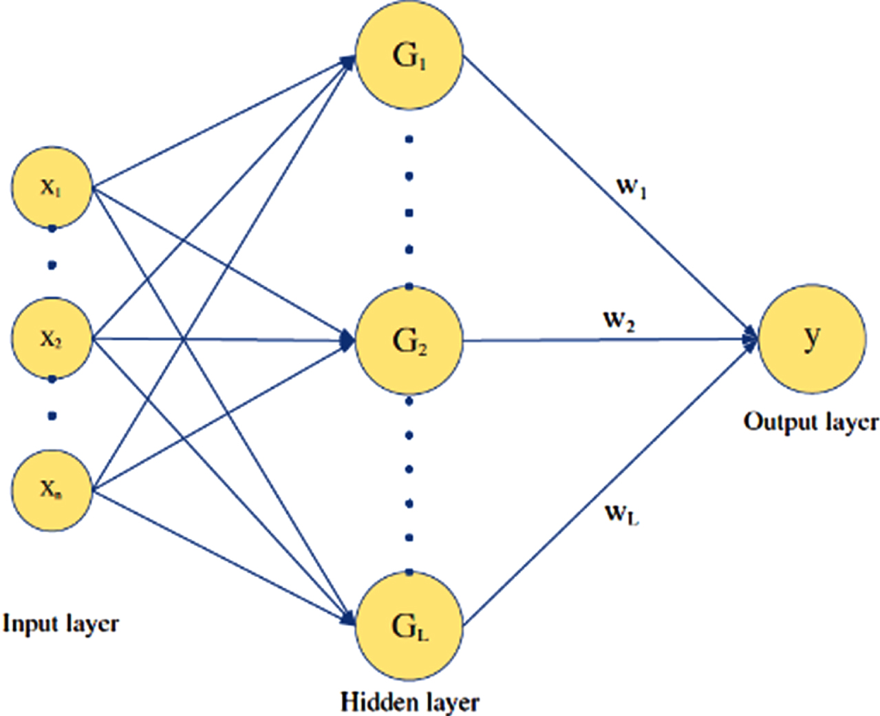
The radial basis function neural network structure.

There are several types of RBFs, such as Gaussian, hardly multiquadric, Inverse multi-quadratic, and Sigmoid functions. The Gaussian RBF is one of the most well-known functions characterized by a center and a spread.

The input layer is a simple part of a network where a node does not run the process. In addition, the node number in the input layer is the same as the variable number [51]. The second layer named hidden seems as the calculator layer, containing radial basis function (RBF) with circular type to find answers. This layer receives the dataset from the first one (input) that uses the RBF to perform a non-linear mapping to the input value. The symmetric function used in RBFNN calculates the distance of a particular input value from a center point. However, there are various types of RBF, including hardly multiquadric, Gaussian, Sigmoid functions, and Inverse multi-quadratic. Gauss RBF has been a well-known function elaborated by spread rate and center [52].

Utilizing the RBF on input vectors, the hidden layer output nodes can be transferred to the output layer with the aggregation of data produced by hidden layer in the simple regression process within the output layer. The RBFNN process can be listed as: 1) determining the radial distance (d_i) between the center (c_i) and input vector (x) for the ith node of RBF in the hidden layer, and, the outcomes (h_i) will be computed by the network (G) with relations presented in following:

$d_{i} = ∥ x - c_{i} ∥$ (1) $h_{i} = G (d_{i} \times σ_{i})$ (2) where σ_i shows the width of i RBF neuron embedded within the hidden layers, and G represents the main function of RBF model. The results of the output layer are specified with Eq. (6): $y = \sum_{i}^{1} w_{i} h_{i}$ (3) where the number of neurons equals one in hidden layer, and weights are defined with w_i among the neurons of output and hidden layers.

2.2 Whale optimization algorithm

The whale optimization algorithm (WOA) was designed based on the hunting prey by creating bubble-net by humpback whales shown in Fig. 2 [53]. In fact, it has been an intelligent swarm-based approach considered to solve the complex optimization problems having continuous domain [54–56]. Seeking prey within multi-dimensional spaces in the swarm, whales will be located as the decision variables, while the objective function is designed to have the minimum distance between whales concerning the position of prey. The time constraint function as locations for a whale is evaluated by the operation steps written as follows [53–57]: (i) shrinkage circling hunt, (ii) exploit phase (as the attack in bubble-net), and (iii) Explore phase (as finding preys). As shown in Fig. 2, when recognizing the prey position, the whale goes to encircle it by moving in 9 steps. This algorithm defines the prey as the most suitable potential solution (target near the best answer) due to having no information on the optimal position of preys in the searching area. For finding the best search candidate every possible attempt is taken into consideration.

Fig. 2

The bubble net created by humpback whale.

Interestingly, other agents try to update their locations adjacent to the best answer that is shown through Fig. 3 [52].

Fig. 3

The spiral updating process [52].

$\vec{D} = | C . {\vec{X}}^{*} (t) - \vec{X} (t) |$ (4) $\vec{X} (t + 1) = {\vec{X}}^{*} (t) - A . \vec{D}$ (5) $A = 2 . a . r - a$ (6) $C = 2 . r$ (7) in which ${\vec{X}}^{*}$ = the global best location, $\vec{X}$ = position of humpback whale, t = recent attempt. Also, a declines linearly between 2 and 0, and r = accidental value distributed normally in [0–1]. The stages are explained in the following:

For the Exploitation phase, the hunting bubble net is defined using Fig. 4 [52]. The same space among the whale positions and preys will be defined by applying a mathematical method that is helix. The hunter positions (in a spiral shape) is tunned after moving [55]:

Fig. 4

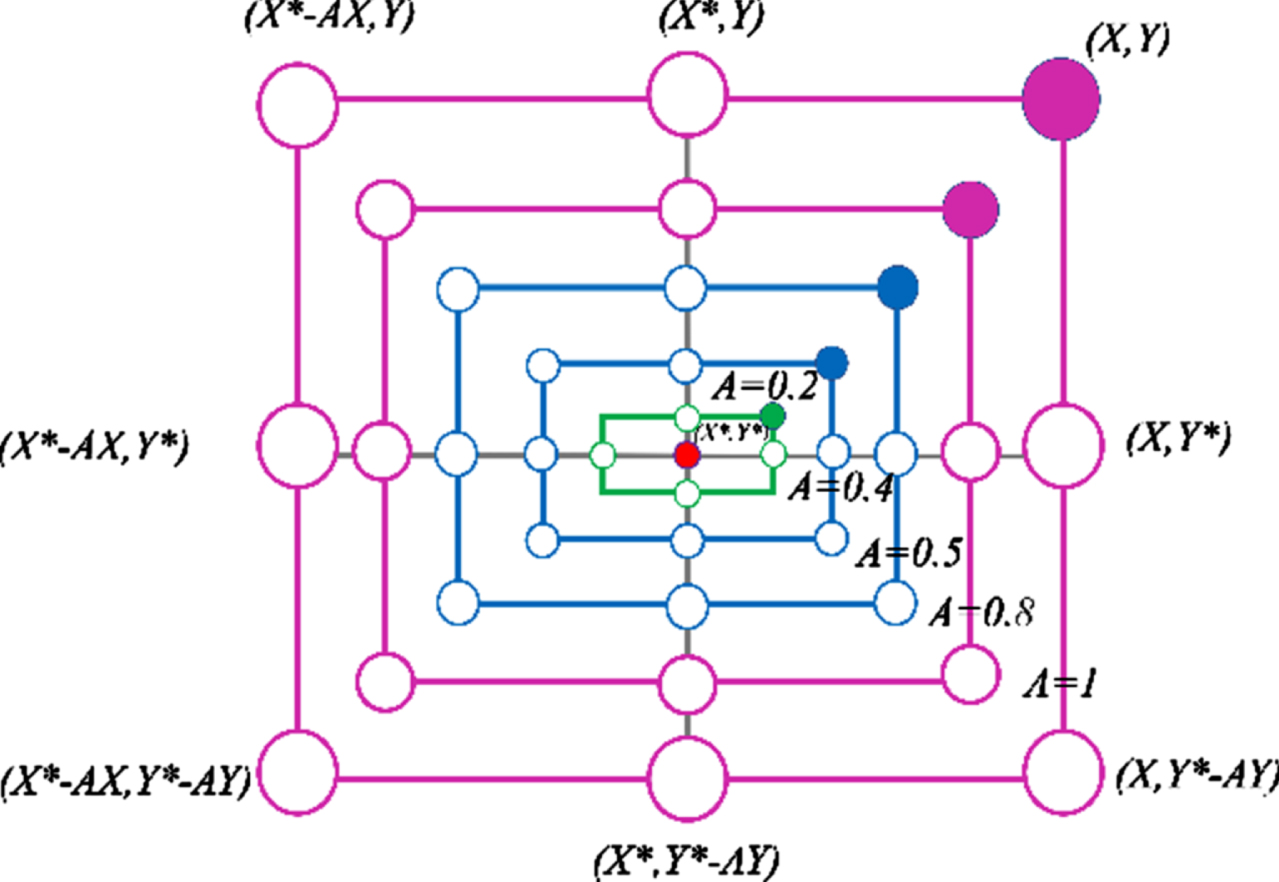
Exploitation phase [52].

$\vec{X} (t + 1) = e^{bk} . cos (2 . pi . k) . {\vec{D}}^{'} (t) + {\vec{X}}^{*} (t)$ (8) ${\vec{D}}^{'} (t) = | {\vec{X}}^{*} (t) - \vec{X} (t) |,$ (9) where b is the fixed value and k shows number as to be arbitrary, b represents the helix shape that is logarithmic, and k shows the accidental value with normal distribution in the range of (–1 to 1).

For exploration phase as shown by Fig. 5 [52], if A< –1 or A > 1, the agent of the search will be dated via a randomly selected whale at elite agent location:

Fig. 5

Exploration phase [52].

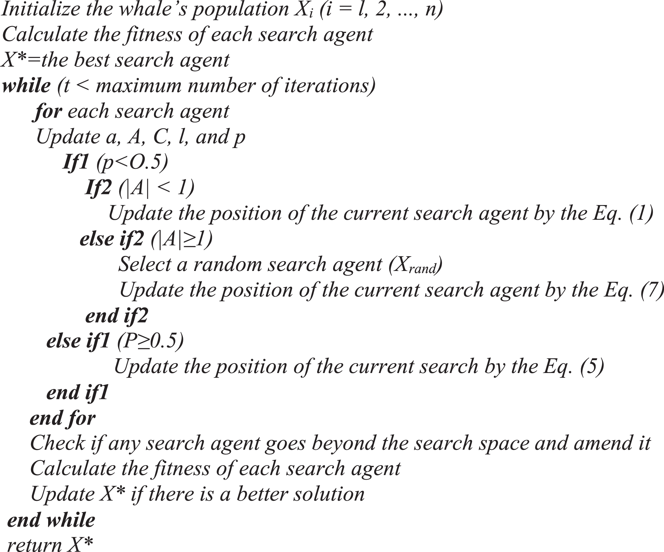
$\vec{X} (t + 1) = \vec{X_{rand}} - A . {\vec{D}}^{'}$ (10) ${\vec{D}}^{''} = | C . \vec{X_{rand}} - \vec{X} (t) |$ (11) where, $C . \vec{X_{rand}}$ shows whales arbitrarily for iterations proposed. In addition, the pseudo-code of WOA has been brought in Fig. 6. Also, for more detail the main reference of WOA is available [50].

Fig. 6

The pseudocode of the WOA algorithm.

2.3 Salp swarm algorithm

The Salp swarm algorithm (SSA), as an intelligent optimizer swarm basis, was inspired by the foraging process of salp swarms [46]. In the struggle for more food sources, these creatures are linked by salp chains, allowing them to quickly communicate and locate food sources [47]. In the Salp School, different salps play different roles: followers and leaders. Followers follow the leader’s instructions and leaders lead the entire population. The final goal of salp is to find the best source of food, indicated as F in the searching space. As with other group basis algorithms, the initial population, consisting of the numbers and location of individuals, will be predefined. Every individual is a prospective solution for the best answer. All solutions’ space has been denoted by U_i that is a two-dimensional matrix. $U_{i} = [\begin{matrix} u_{1}^{1} & \dots & u_{d}^{1} \\ ⋮ & ⋱ & ⋮ \\ u_{1}^{n} & \dots & u_{d}^{n} \end{matrix}]$ (12)

Continuously, the initialized swarm of salps will be updated by processing mathematic operations within the model, in which followers and leaders track the various equations. However, a leader plays a main role in searching food and navigation, as updated in Eq. (10): $u_{m}^{1} = {\begin{matrix} F_{m} + c_{1} (({kb}_{m} - {jb}_{m}) c_{2} + {jb}_{m}) c_{3} ⩾ 0 \\ F_{m} - c_{1} (({kb}_{m} - {jb}_{m}) c_{2} + {jb}_{m}) c_{3} ⩽ 0 \end{matrix}$ (13) where the leader position in the dimension m is shown by $u_{m}^{1}$ ; F_m is the source position of food for the dimension m, jb_m and kb_m shows, respectively, the power and upper boundaries of the dimension m. c₂ and c₃ variables as accidental magnitudes from 0 to 1, determining the direction of later search in the search domain toward+inf. or –inf. and search step size. The variable, also, creating a balance between exploration space and exploitation depth is c₁. Considerably, c₁ declines with the iteration number increasing that is obtained by Eq. (11): $c_{1} = 2 e^{- {(\frac{4 j}{J})}^{2}}$ (14) wherein j and J stand for, respectively, number of current and maximum iteration. For a follower salp, the given position will be upgraded as shown in in Eq. (12): $u_{m}^{i} = \frac{1}{2} (u_{m}^{i} + u_{m}^{i - 1})$ (15) where, $u_{m}^{i}$ shows the ith salp position for the dimension m and i≥2. Fig. 4 has shown the Pseudo code of SSA.

2.4 Data preparation to train models

Modeling the mechanical properties of HPC mixtures via RBFNN would be accompanied with metaheuristic algorithms to generate WORBF and SSRBF hybrid models. Actually, this study examined a dataset containing 181 HPC samples [56] including fine/coarse aggregates, water/binder ratio, air agent, fly-ash, and superplasticizer. Notably, the CS and SL measurements were performed on the 28th day of the concrete age. Table 1 provides a summary of relevant data from a statistical point of view in which CS shows the compressive strength, SL is slump, W/B is the ratio of water to binder, W is water, S/A shows ratio of the weight of fine aggregate to that of all aggregate, SF silica-fume, FA fly-ash, AE content of air-entraining agent, SP shows the superplasticizer. Mentioned dataset can be divided into two types: i) independent variables, which are the components mixed to create the HPC blend ii) dependent variables of mechanical properties: compressive strength and slump features affected by the introduced independent data i. Therefore, all data is fed in hybrid WORBF and SSRBF models as a training and validation phases and then tested. In this regard, the above three stages are performed as subphases of the training phase, too. Specifically, 70% of the mixtures’ data are chosen in the train phase and another 30% is used in the same proportion in the test and validation phases. Fig. 7 shows the whole data used to train models. The coupling mechanism of optimizers SSA and WOA with RBF to generate holistic frameworks of SSRBF and WORBF has been revealed through Fig. 8.

Table 1
Summary statistical report of model inputs

Parameter CS Slump W/B W S/A FA AE SF SP

Unit (MPa) (mm) (%) (kg/m3) (%) (%) (kg/m3) (%) (kg/m3)

Max 123 260 45 180 53 20 0.08 25 36.5

Min 38 95 18 140 35 0 0 0 1.89

Ave 74.17 202.73 31.17 162.13 42.15 5.8 0.03 6.44 10.93

St. dev. 26.64 25.93 8.77 12.12 5.37 8.03 0.03 8.43 8.63

Median 63 205 30 160 42 0 0.038 0 8

Parameter	CS	Slump	W/B	W	S/A	FA	AE	SF	SP
Max	123	260	45	180	53	20	0.08	25	36.5
Min	38	95	18	140	35	0	0	0	1.89
Ave	74.17	202.73	31.17	162.13	42.15	5.8	0.03	6.44	10.93
St. dev.	26.64	25.93	8.77	12.12	5.37	8.03	0.03	8.43	8.63
Median	63	205	30	160	42	0	0.038	0	8

Fig. 7

Input data used to train models including: a) air entraining, b) fly-ash, c) ratio of the weight of fine aggregate to the weight of all aggregate, d) superplasticizer, e) water, f) water to binder ratio, g) compressive strength, and h) slump flow.

Fig. 8

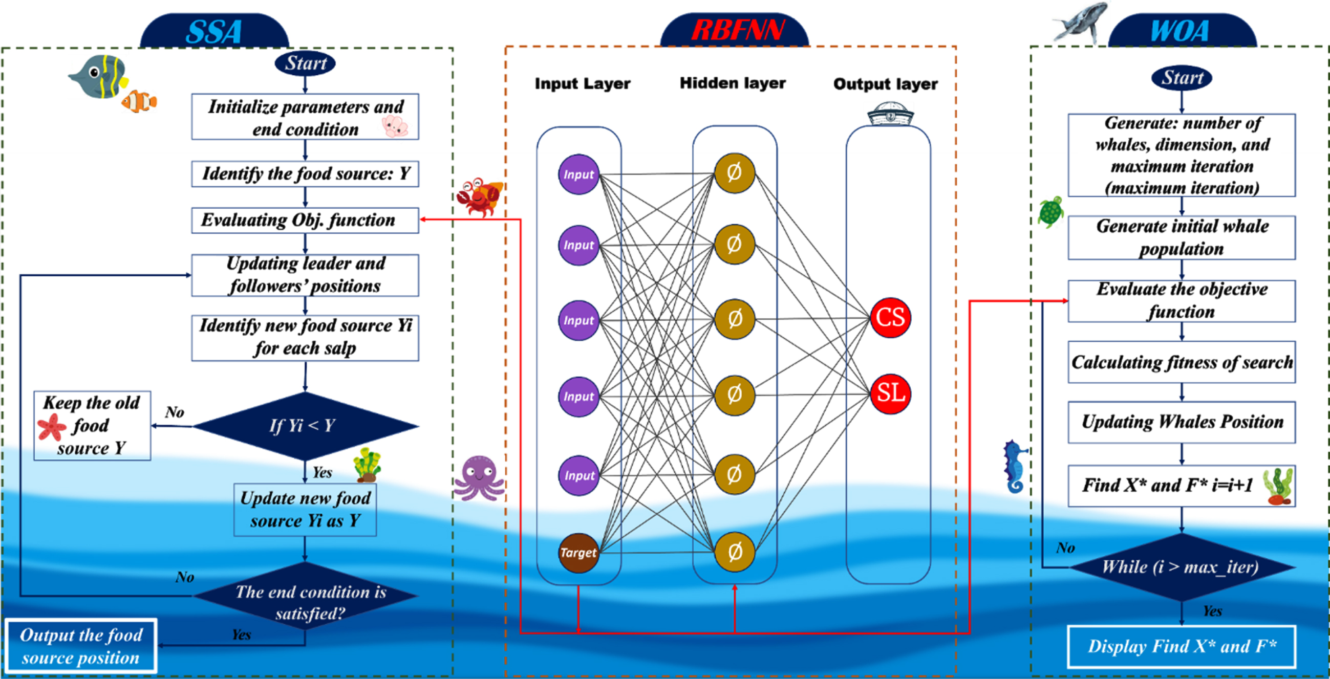
Flowchart of developed hybrid models: WORBF and SSRBF.

2.5 Evaluation of developed hybrid models

For assessing the performance of WORBF and SSRBF in the prediction of compressive strength and slump rate of high-performance concrete (HPC) samples, various types of evaluation indicators are shown through Table 2. In Table 2, t_n represents the measured numbers of CS and SL and the averages are indicated via $\bar{t}$ ; the predicted values have been shown with p_N with average of $\bar{p}$ . The number of HPC mixtures for the training and testing phases are indicated by n_train and n_test, respectively.

Table 2
Evaluating indices for analyzing the proposed frameworks

Criteria Nomenclatures Equation Assessment

Variance account factor VAF $(1 - \frac{var (t_{n} - y_{n})}{var (t_{n})}) * 100$ (6) Higher is desirable

Mean absolute error MAE $\frac{1}{N} \sum_{n = 1}^{N} | p_{n} - t_{n} |$ (7) Lower is desirable

Root mean squared error RMSE $\sqrt{\frac{1}{N} \sum_{n = 1}^{N} {(p_{n} - t_{n})}^{2}}$ (8) Lower is desirable

Pearson’s correlation coefficient R² $(\frac{\sum_{n = 1}^{N} (t_{n} - \bar{t}) (p_{n} - \bar{p})}{\sqrt{[\sum_{n = 1}^{N} {(t_{n} - \bar{p})}^{2}] [\sum_{n = 1}^{N} {(p_{n} - \bar{p})}^{2}]}})$ 2 (9) Higher is desirable

Statistical parameter including the various indices OBJ $(\frac{n_{train} - n_{test}}{n_{train} + n_{test}}) \frac{{RMSE}_{train} + {MAE}_{test}}{R_{train}^{2} + 1} + (\frac{2 n_{train}}{n_{train} + n_{test}}) \frac{{RMSE}_{test} - {MAE}_{test}}{R_{test}^{2} + 1}$ (10) Lower is desirable [33]

Criteria	Nomenclatures	Equation	Assessment
Variance account factor	VAF	$(1 - \frac{var (t_{n} - y_{n})}{var (t_{n})}) * 100$ (6)	Higher is desirable
Mean absolute error	MAE	$\frac{1}{N} \sum_{n = 1}^{N} \| p_{n} - t_{n} \|$ (7)	Lower is desirable
Root mean squared error	RMSE	$\sqrt{\frac{1}{N} \sum_{n = 1}^{N} {(p_{n} - t_{n})}^{2}}$ (8)	Lower is desirable
Pearson’s correlation coefficient	R²	$(\frac{\sum_{n = 1}^{N} (t_{n} - \bar{t}) (p_{n} - \bar{p})}{\sqrt{[\sum_{n = 1}^{N} {(t_{n} - \bar{p})}^{2}] [\sum_{n = 1}^{N} {(p_{n} - \bar{p})}^{2}]}})$ 2 (9)	Higher is desirable
Statistical parameter including the various indices	OBJ	$(\frac{n_{train} - n_{test}}{n_{train} + n_{test}}) \frac{{RMSE}_{train} + {MAE}_{test}}{R_{train}^{2} + 1} + (\frac{2 n_{train}}{n_{train} + n_{test}}) \frac{{RMSE}_{test} - {MAE}_{test}}{R_{test}^{2} + 1}$ (10)	Lower is desirable [33]

3 Results and discussions

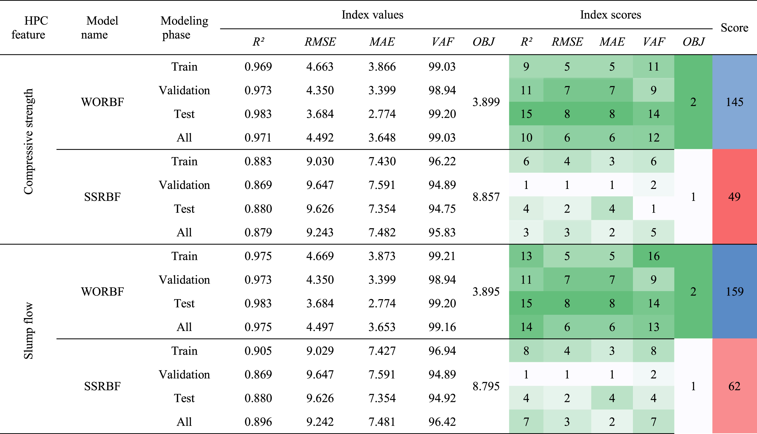
The modeling process was conducted for the developed frameworks WORBF and SSRBF. In fact, by feeding the input data of HPC ingredients as well as the compressive strength and slump flow rates as targets to models, training operation was done to predict the mentioned target numbers with similar inputs. Actually, the hardness properties of samples were surveyed in four different conditions as brought in Table 3. The indices aforementioned assessed the results of models in four stages of training, validation, testing, and considering all of the data. In addition, in the score part of the table, the mentioned results of indicators were ranked and then summed to generate the final scores for each defined condition. As shown in Table 3, modeling the slump flow of HPC samples was done with better results. However, in the training phase of modeling CS by WOA optimizer, the correlation index of R² was calculated at 96.9 percent that was 11% more than that of SSRBF. The high-accuracy modeling based on the RMSE index was done by WORBF with 3.684 mm (and MPa) for both concrete aspects. On the other hand, the WOA optimizer could tune the RBFNN to reach the prediction of CS and SL according to the MAE index. In testing phase the minimum rate of MAE is diagnosed for all of models between various stages that 2.77 mm (and MPa) was the minimum rate of error seen in simulations. Assessment of the models using VAF proved the fact that WORBF was successful in prediction. With this respect, in the modeling the slump rate of HPC samples, the training phase could receive a 99.21 rate that was 3.52% more than the SSRBF result. Despite the fact that referred four indicators had four stages of modeling, the OBJ index is calculated based on the results of other criteria, so can show a comprehensive view of the models’ ability to appraise the target features of HPC. Regarding the results, the SSA was not prosperous compared to WOA. For estimating the SL factor WORBF could do a better job with the rate of 3.89 that was 139% more than that of SSRBF. While for estimation of CS the difference was calculated at 140% that SSRBF had an 8.79 mm error. Relied on the evaluative results of five assessment criteria, the ranking of each index was done and they were summed to show the total scores in the last column. Based on the total scores of the models, WOA has been efficient in tunning RBFNN with 66% and 61% discrepancies to appraise the CS and SL properties of HPC samples respectively.

Table 3
The results of evaluation criteria and scoring models

Nevertheless, WORBF and SSRBF models to estimate the target values of compressive strength and slump flow used same data inputs as ingredients and measured CS and SL. To survey the interaction of them rather to each other, Fig. 9 has indicated the correlation index of R² between mentioned parameters and also the target values of CS and SL. Regarding the correlation rates seen in Fig. 9, the highest R² can be found among compressive strength with water to binder ratio (W/B) in negative direction, superplasticizer and silica-fume in positive way which are dedicated with red and blue box, respectively. On the other side, for slump as expected, the water to binder ratio (W/B) plays the main role then fine aggregate to total aggregates ratio. According to the ingredient used in HPC compounds, the roles of each additive is clear with the aid of Fig. 9. For example, except for silica-fume and superplasticizer, other remaining materials have reduced the stability and cohesion of concrete then led to decreasing compressive strength

Fig. 9

Correlation of inputs and targets used in models.

Fig. 10

Counter map of: a) water, superplasticizer, CS, b) water, superplasticizer, SL, c) water/binder, fine aggregate/total aggregate, SL.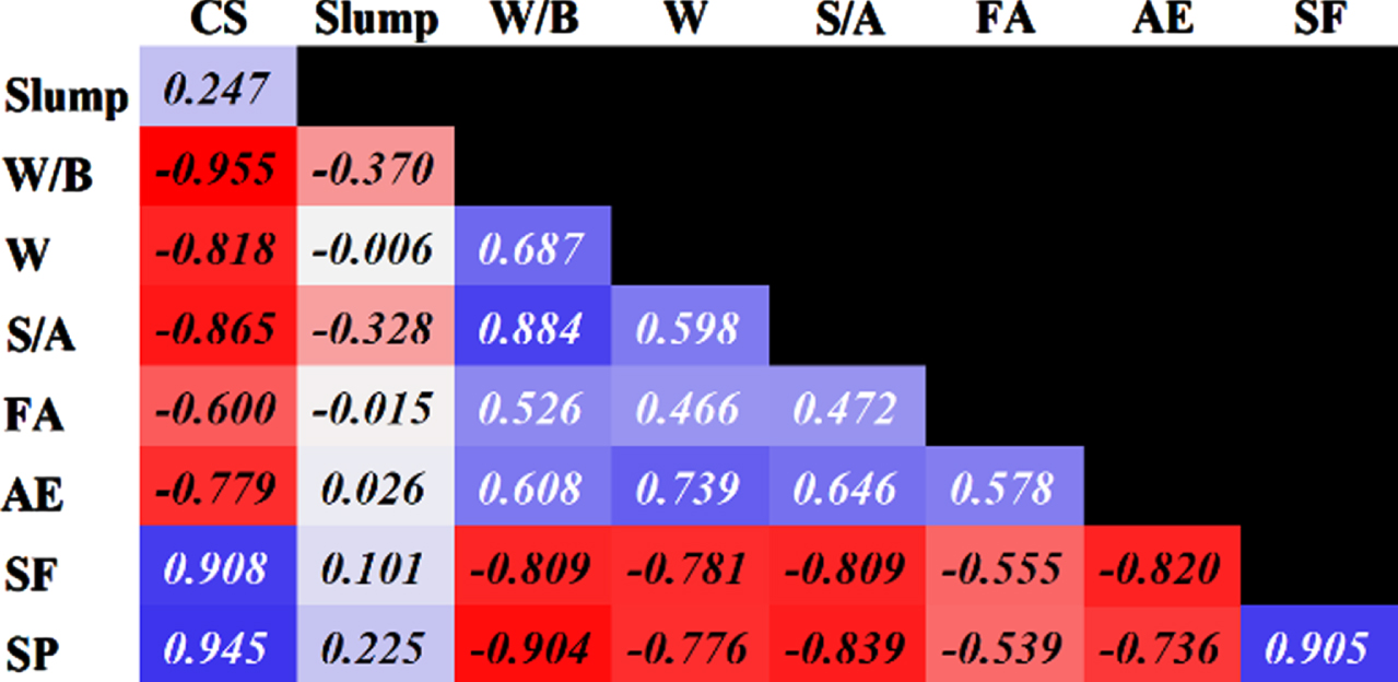

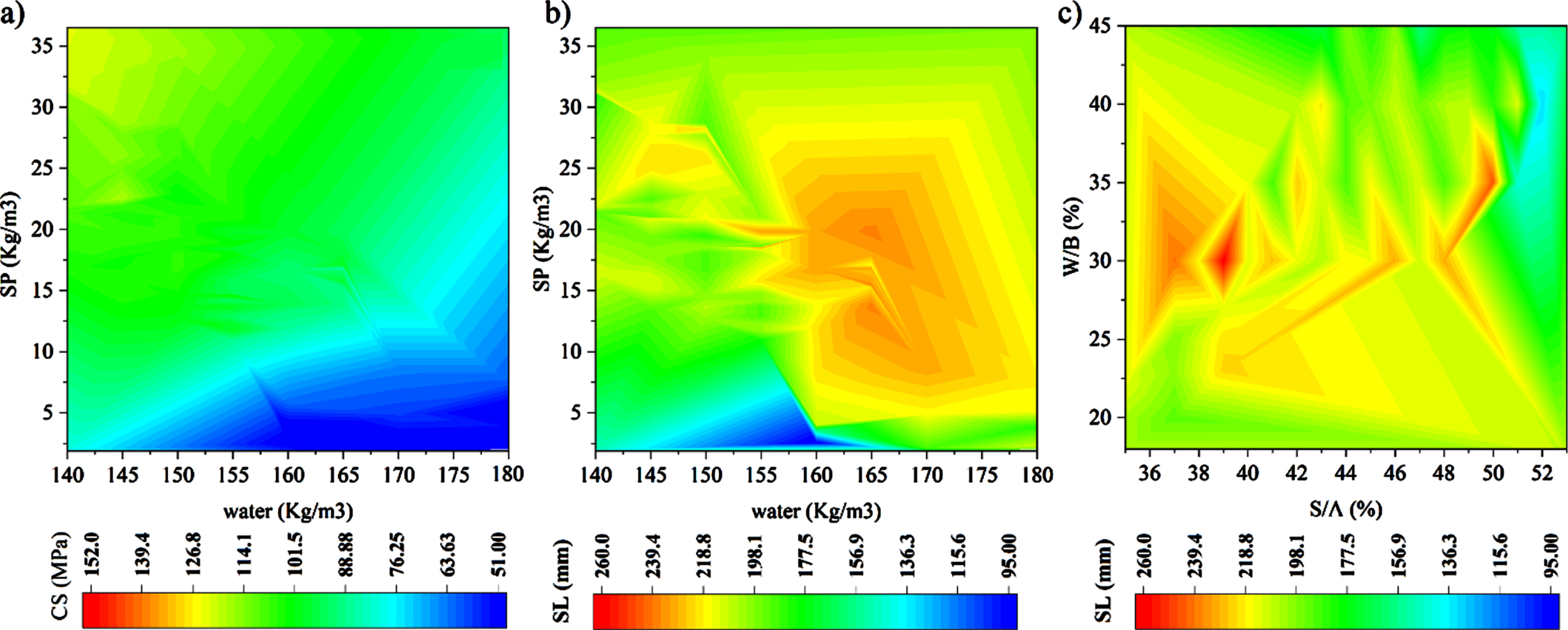
rate. Additionally, to scrutinize the impacts of efficient materials with high correlation, Fig. 10 has presented the behavior of mixing these ingredients and the response of CS and SL.

Based on Fig. 10 for compressive strength (a), the roles of superplasticizer and water is clearly obvious that by increasing water and decreasing SP, the CS would decline. Despite the reduction of CS with water increasing, the covering role of SP could enhance the CS rate. Moreover, considering SL with the effects of same materials (b), the lowest SL has been happened at the lowest rate of SP. In Fig. 10 (c), the impacts of W/B and S/A on SL simultaneously, cannot prove a same pattern but in a certain zone of W/B (25% –37.5%), the SL has been topped to its highest rate. Nevertheless, by increasing S/A and W/B linearly, the S/A could prevail the effects of water and has reduced the slump of HPC.

Modeling the geomechanical features of HPC samples is important to survey in terms of error rates that are defined the difference between predicted and measured value. To this end, Fig. 11 has shown the performance of each models to estimate the CS and SL factors. Based on Fig. 11, the modeling by WOA optimizer has been prospering compared to SSA that the points of plots can confirm this fact. In estimation of CS by WORBF (a) gathering points around the fitting line is more than SSRBF (b). To better understand the modeling process, also the equations of fitting line can assist to know how the CS points were modeled. In this regard, the slope of fitting line relevant to WORBF is 0.97 while that of SSRBF has been calculated 0.88, with 9.3% difference. In addition, a near distance between bisector line of Y = X and fitting line in WORBF shows a better simulation of compressive strength rates rather to SSRBF. Besides, the distribution of CS points in SSRBF is more broad than WORBF. On the other side, modeling SL was done at the similar condition and the WOA could tune the RBFNN better than SSA. In estimating slump rates, WORBF by reducing the errors better than SSRBF, gathered the SL points at better conditions and more closer to the fitting line that the RMSE of earlier model was calculated about 106 percent more than latter one. The slope of fitting line equation, also, was a computed 0.91 for WORBF while 0.88 for another model, with 3.3 percent difference.

Fig. 11

Measured (target) values against the predicted values modeled by: a) WORBF (estimating CS), b) SSRBF (estimating CS), c) WORBF (estimating SL), and d) SSRBF (estimating SL).

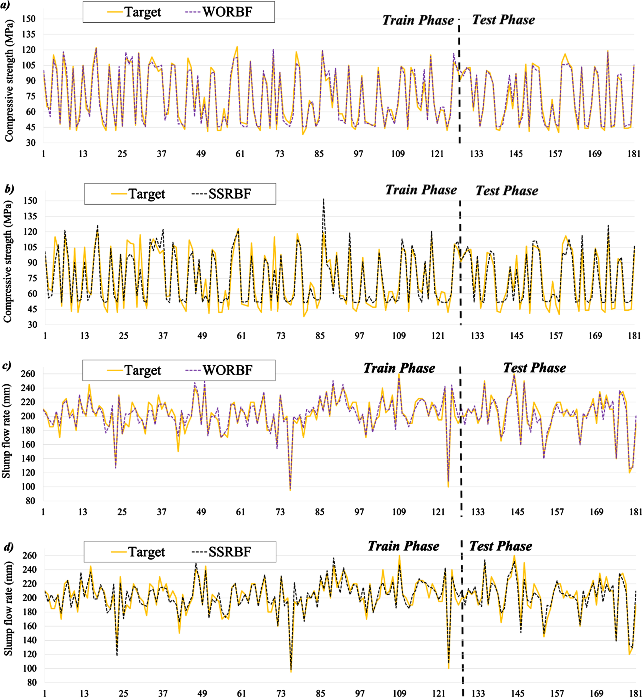
To bolding the the differences of modeling rates with measured (as targets), Fig. 12 has attempted to show the gaps for each HPC samples. As shown in Fig. 12, the coincidence of model lines with measured lines are at acceptable conditions, while there are some mismatch between them. The main gaps can found in modeling CS by SSRBF (b) that in testing phase most of errors has been cured while in estimation of SL there are cases of overestimation and underestimation. For CS modeling, the highest errors can be found in SSRBF especially for mixture #86 that in WORBF (a) it is placed on the target line. Generally, the modeling results in testing phase has been improved by considering the gaps among dashed line of model and target lines. Also the SL of samples were modeled with gaps but in this case, the gaps are rarely found to be large. With this respect, there can be found positions in SSRBF that have exceeded the target line. For example, in sample #54 that is leaved in the training stage, the SL has been estimated higher than target line. But generally, the modeling of slump flow with to developed models of WORBF and SSRBF has been simulated better than compressive strength factor.

Fig. 12

Error percentage rates embedded in CS and SL modeled by: a) WORBF (estimating CS), b) SSRBF (estimating CS), c) WORBF (estimating SL) and d) SSRBF (estimating SL).

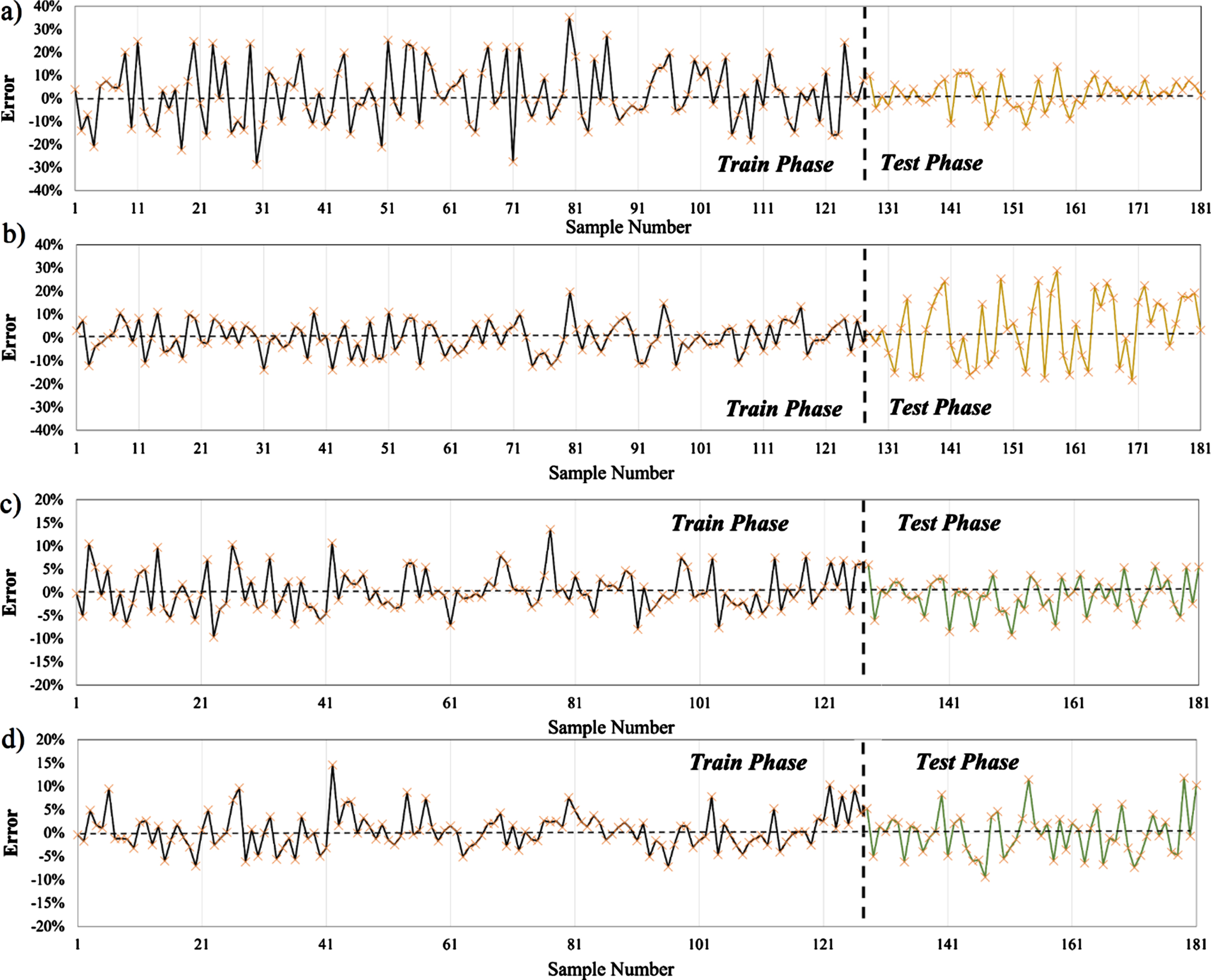
For enlarging the mentioned gaps between measured and modeled target values, the errors should be provided to give us a detailed view of modeling process for each sample. In this regard, Fig. 13, indicates the capability of models in overcoming errors in modeling operation. In light of analyzing performance of models in removing errors, considering the error threshold of similar concrete characteristic would help us. With considering this fact in Fig. 13, the CS charts has the error range of –40% to+40% and for SL –20% to+20%. This fact can prove that the error limit of CS is twice SL.

Fig. 13

Error histogram plus the normal distribution curves for: a) Training phase in estimating CS, b) Testing phase in estimating CS, c) Training phase in estimating SL, and d) Testing phase in estimating SL.

According to Fig. 13 in estimation of CS, two various trend in data distribution can be found. Firstly, for WORBF, the training phase has led to reduce the errors in testing phase, showing the appreciable training process. While the inverse circumstances can be seen for SSRBF in which the error domain of testing phase is lower than training phase. The high-error HPC samples modeled by WORBF are seen in mixtures #95 with 14.70% error, #117 with 13.4% error, #158 with 13.74% error while similar samples in SSRBF was modeled with 13.17%, 2.94%, 28.89% error. Similar event can be seen in estimation of slump flow diagrams.

Based on Fig. 13(c), the WOA has been successful to train the model RBFNN to generate the SL rates. Because of results that in testing phase the error rates are diminished outstandingly from averagely 2.97% to 3.59%. SSA optimizer also could do better job but in testing phase the error rates went up for the samples that in WORBF had better results.

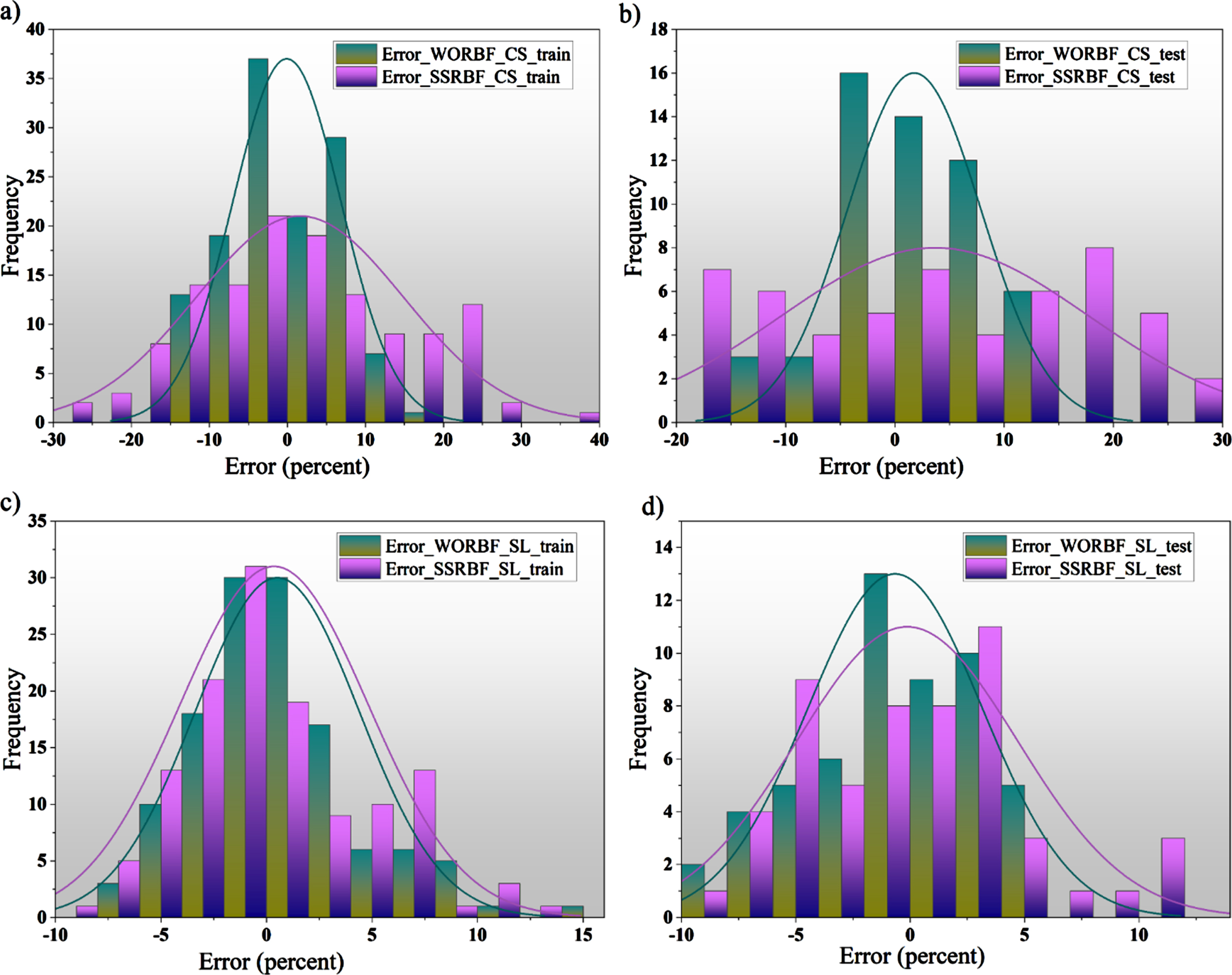
Distribution of errors are so important that in Fig. 14 using the normal distribution curve of errors for each models can give us the ability of models in dealing with errors. As can be seen from the Figs. 14-a and 14-b, to appraise the CS values, the WOA has minimized the errors near to the zero level in training stage while SSA optimizer has distributed the errors among broadly leading to flattening the normal distribution curve of errors. In opposite state, the normal distribution curve of errors for WORBF is sharpened and resembles to bell. For testing phases, however this story runs true and error distribution of SSRBF do not follow the normal distribution. Nonetheless, in estimation of SL, both models have worked alike compared to CS and even in training phase, the SSA could manage the errors better than WOA. But in testing phase WORBF appears to play better role in controlling errors.

4 Conclusion

Examining the properties of High-Performance Concrete (HPC) has been a big challenge due to the highly heterogeneous relationships and coherence among several constituents. The employment of some specific additives such as superplasticizer, silica-fume and fly-ash as eco-friendly components in mixtures benefits the concrete to improve its physical features. Although machine learning approaches are utilized broadly to solve problems, employing models solitarily to estimate the mechanical features of concrete in similar researches has caused in reducing the accuracy and lift the cost and complexities of computational networks. Therefore, in this study a Radial Basis Function Neural Network (RBFNN) was developed with two optimization algorithms of Whale Optimization Algorithm (WOA) and Salp Swarm Algorithm (SSA) in order to precisely model the mechanical characteristics of HPC mixtures including compressive strength (CS) and slump (SL). The hybrid models of WORBF and SSRBF could reproduce the SL and CS rates of 181 HPC compounds based on the data of ingredients feeding the models. By generating results in the training phase of modeling CS using WORBF, the correlation index of R2 was calculated 96.9 percent that was 11% more than that of SSRBF. The high-accuracy modeling based on RMSE index was done by WORBF with 3.684 mm (and MPa) for both concrete aspects. On the other hand, the WOA optimizer could tune the RBFNN to reach prediction of CS and SL according to MAE index. In testing phase the minimum rate of MAE was diagnosed for all of models between various stages that 2.77 mm (and MPa) was the minimum rate of error seen in simulations. In addition, based on OBJ indicator encompassing various types of indicators, the SSA was not prosperous compared to WOA. For estimating SL factor WORBF could do better job with the rate of 3.89 that was 139% more than that of SSRBF. Moreover, the WOA minimized the errors near to the zero level in training stage while SSA optimizer distributed the errors among broadly leading to flattening the normal distribution curve of errors. In opposite state, the normal distribution curve of errors for WORBF was sharpened and resembled to the shape of a bell. For testing phases, however error distribution of SSRBF did not follow the normal distribution. Nonetheless, in estimation of SL, both models worked alike compared to CS and even in training phase, the SSA could manage the errors better than WOA. But in testing phase, WORBF appeared to play better role in controlling errors.

To sum up, most of results affirmed that both models were capable to generate the acceptable outcomes while in some cases the WORBF appeared better than SSRBF. Generally, using such methods instead of experimental ways can increase the profitability of researches when using the physical appliances seems costly; especially, using high-accuracy models has enhanced the applicability of smart models in reducing the costs and energy loss and definitely increasing the accuracy of estimation. However, some limitations can be happened for other predictions when employing various dosages of concrete components, or using experimental data having probable error in gauging each constituent to develop a predictive framework with an aim of modeling mechanical features of other concrete mixtures.

References

Neville

and Aïtcin

P.-C.

, High performance concrete— An overview, Mater Struct 31(2) (1998), 111–117. doi: 10.1007/BF02486473.

Leung

C.K.Y.

Concrete as a building material, Encycl Mater Sci Technol (2011), pp. 1471’1479.

Pala

, Özbay

, Öztas

and Yuce

M.I

, Appraisal of long-term effects of fly ash and silica fume on compressive strength of concrete by neural networks, Constr Build Mater 21(2) (2007), 384–394. doi: 10.1016/j.conbuildmat.2005.08.009.

Hassan

and Wille

, Experimental impact analysis on ultra-high performance concrete (UHPC) for achieving stress equilibrium (SE) and constant strain rate (CSR) in Split Hopkinson pressure bar (SHPB) using pulse shaping technique, Constr Build Mater 144 (2017), 747–757. doi: 10.1016/j.conbuildmat.2017.03.185.

Golewski

G.L.

, Green concrete composite incorporating fly ash with high strength and fracture toughness, J Clean Prod 172 (2018), 218–226.

Jalal

, Pouladkhan

, Harandi

O.F.

and Jafari

, Comparative study on effects of Class F fly ash, nano silica and silica fume on properties of high performance self compacting concrete, Constr Build Mater 94(90), 104, 2015.

Kurt

, Kotan

, Gül

M.S.

, Gül

and Aydin

A.C.

, The effect of blast furnace slag on the self-compactability of pumice aggregate lightweight concrete, Sadhana 41(2) (2016), 253–264.

Güneyisi

, Gesoglu

, Al-Goody

and İpek

, Fresh and rheological behavior of nano-silica and fly ash blended self-compacting concrete, Constr Build Mater 95 (2015), 29–44.

Dey

, Miyani

and Sil

, Application of artificial neural network (ANN) for estimating reliable service life of reinforced concrete (RC) structure bookkeeping factors responsible for deterioration mechanism, Soft Comput 24(3) (2020), 2109–2123. doi: 10.1007/s00500-019-04042-y.

10.

Nakata

I.M.

, Fernández

F.G.

, Carrillo

A.T.

, Haro

P.E.

, Pinaud

L.A.

, Application of the Monte Carlo method to estimate the uncertainty in the compressive strength test of high-strength concrete modelled with a multilayer perceptron, Rev La Constr 17(2) (2018), 319–329.

11.

Yan

and Shi

, Prediction of elastic modulus of normal and high strength concrete by support vector machine, Constr Build Mater 24(8) (2010), 1479–1485. doi: 10.1016/j.conbuildmat.2010.01.006.

12.

Shariati

et al., A novel hybrid extreme learning machine–grey wolf optimizer (ELM-GWO) model to predict compressive strength of concrete with partial replacements for cement, Eng Comput 2020. doi: 10.1007/s00366-020-01081-0.

13.

Lai

and Serra

, Concrete strength prediction by means of neural network, Constr Build Mater 11(2) (1997), 93–98. doi: 10.1016/S0950-0618(97)00007-X.

14.

H.-G.

and Wang

J.-Z.

, Prediction of compressive strength of concrete by neural networks, Cem Concr Res 30(8) (2000), 1245–1250. doi: 10.1016/S0008-8846(00)00345-8.

15.

Öztas

, Pala

, Özbay

, Kanca

, Çlar

and Bhatti

M.A.

, Predicting the compressive strength and slump of high strength concrete using neural network, Constr Build Mater 20(9) (2006), 769–775. doi: 10.1016/j.conbuildmat.2005.01.054.

16.

Słoński

, A comparison of model selection methods for compressive strength prediction of high-performance concrete using neural networks, Comput Struct 88(21–22) (2010), 1248–1253. doi: 10.1016/j.compstruc.2010.07.003.

17.

Bui

D.-K.

, Nguyen

, Chou

J.-S.

, Nguyen-Xuan

and Ngo

T.D.

, A modified firefly algorithm-artificial neural network expert system for predicting compressive and tensile strength of high-performance concrete, Constr Build Mater 180 (2018), 320–333. doi: 10.1016/j.conbuildmat.2018.05.201.

18.

Kasperkiewicz

, Racz

and Dubrawski

, HPC Strength Prediction Using Artificial Neural Network, J Comput Civ Eng 9(4) (1995), 279–284. doi: 10.1061/(ASCE)0887-3801(1995)9:4(279).

19.

Yaprak

, Karacı

and Demir

İ.

, Prediction of the effect of varying cure conditions and w/c ratio on the compressive strength of concrete using artificial neural networks, Neural Comput Appl 22(1) (2013), 133–141. doi: 10.1007/s00521-011-0671-x.

20.

Sarıdemir

, Prediction of compressive strength of concretes containing metakaolin and silica fume by artificial neural networks, Adv Eng Softw 40(5) (2009), 350–355. doi: 10.1016/j.advengsoft.2008.05.002.

21.

Han

, Gui

, Xu

and Lacidogna

, A generalized method to predict the compressive strength of high-performance concrete by improved random forest algorithm, Constr Build Mater 226 (2019), 734–742. doi: 10.1016/j.conbuildmat.2019.07.315.

22.

Rafiei

M.H.

, Khushefati

W.H.

, Demirboga

and Adeli

, Supervised Deep Restricted Boltzmann Machine for Estimation of Concrete., ACI Mater J 114(2) (2017);.

23.

Feng

D.-C.

et al., Machine learning-based compressive strength prediction for concrete: An adaptive boosting approach, Constr Build Mater 230 (2020), 117000. doi: 10.1016/j.conbuildmat.2019.117000.

24.

Chou

J.-S.

, Chiu

C.-K.

, Farfoura

and Al-Taharwa

, Optimizing the prediction accuracy of concrete compressive strength based on a comparison of data-mining techniques, J Comput Civ Eng 25(3) (2011), 242–253.

25.

Erdal

H.I.

, Karakurt

and Namli

, High performance concrete compressive strength forecasting using ensemble models based on discrete wavelet transform, Eng Appl Artif Intell 26(4) (2013), 1246–1254. doi: 10.1016/j.engappai.2012.10.014.

26.

Anyaoha

, Zaji

and Liu

, Soft computing in estimating the compressive strength for high-performance concrete via concrete composition appraisal, Constr Build Mater 257 (2020), 119472. doi: 10.1016/j.conbuildmat.2020.119472.

27.

Young

B.A.

, Hall

, Pilon

, Gupta

and Sant

, Can the compressive strength of concrete be estimated from knowledge of the mixture proportions? New insights from statistical analysis and machine learning methods, Cem Concr Res 115 (2019), 379–388. doi: 10.1016/j.cemconres.2018.09.006.

28.

Asteris

P.G.

, Skentou

A.D.

, Bardhan

, Samui

and Pilakoutas

, Predicting concrete compressive strength using hybrid ensembling of surrogate machine learning models, Cem Concr Res 145 (2021), 106449.

29.

Yeh

I.-C.

and Lien

L.-C.

, Knowledge discovery of concrete material using genetic operation trees, Expert Syst Appl 36(3) (2009), 5807–5812.

30.

Gandomi

A.H.

and Alavi

A.H.

, A new multi-gene genetic programming approach to nonlinear system modeling. Part I: materials and structural engineering problems, Neural Comput Appl 21(1) (2012), 171–187.

31.

Mousavi

S.M.

, Gandomi

A.H.

, Alavi

A.H.

and Vesalimahmood

, Modeling of compressive strength of HPC mixes using a combined algorithm of genetic programming and orthogonal least squares, Struct Eng Mech An Int J 36(2) (2010), 225–241.

32.

Mousavi

S.M.

, Aminian

, Gandomi

A.H.

, Alavi

A.H.

and Bolandi

, A new predictive model for compressive strength of HPC using gene expression programming, Adv Eng Softw 45(1) (2012), 105–114.

33.

Pazouki

, Golafshani

E.M.

, Behnood

Predicting the compressive strength of self-compacting concrete containing Class F fly ash using metaheuristic radial basis function neural network, Struct Concr 2021. doi: 10.1002/suco.202000047.

34.

Gao

and Jun-Wei

, Estimation of pile settlement applying hybrid radial basis function network with BBO, ALO, and GWO optimization algorithms, J Appl Sci Eng 25(6) (2022), 1031–1044.

35.

Broomhead

D.S.

, Lowe

Radial basis functions, multi-variable functional interpolation and adaptive networks, Royal Signals and Radar Establishment Malvern (United Kingdom), 1988.

36.

Moodi

, Ghasemi

and Mousavi

S.R.

, Estimating the compressive strength of rectangular fiber reinforced polymer–confined columns using multilayer perceptron, radial basis function, and support vector regression methods, J Reinf Plast Compos 41(3–4) (2022), 130–146.

37.

Topcu

İ.B.

and Sarıdemir

, Prediction of compressive strength of concrete containing fly ash using artificial neural networks and fuzzy logic, Comput Mater Sci 41(3) (2008), 305–311. doi: 10.1016/j.commatsci.2007.04.009.

38.

Zarandi

M.H.F.

, Türksen

I.B.

, Sobhani

and Ramezanianpour

A.A.

, Fuzzy polynomial neural networks for approximation of the compressive strength of concrete, Appl Soft Comput 8(1) (2008), 488–498.

39.

Atici

, Prediction of the strength of mineral admixture concrete using multivariable regression analysis and an artificial neural network, Expert Syst Appl 38(8) (2011), 9609–9618. doi: 10.1016/j.eswa.2011.01.156.

40.

Chou

J.-S.

and Tsai

C.-F.

, Concrete compressive strength analysis using a combined classification and regression technique, Autom Constr 24 (2012), 52–60.

41.

Chou

J.-S.

and Pham

A.-D.

, Enhanced artificial intelligence for ensemble approach to predicting high performance concrete compressive strength, Constr Build Mater 49 (2013), 554–563.

42.

Tien Bui

, Abdullahi

M.M.

, Ghareh

, Moayedi

and Nguyen

, Fine-tuning of neural computing using whale optimization algorithm for predicting compressive strength of concrete, Eng Comput 37(1) (2021), 701–712.

43.

Sarir

, Chen

, Asteris

P.G.

, Armaghani

D.J.

and Tahir

M.M.

, Developing GEP tree-based, neuro-swarm, and whale optimization models for evaluation of bearing capacity of concrete-filled steel tube columns, Eng Comput 37(1) (2021), 1–19.

44.

Zhao

, Nguyen

, Nguyen-Thoi

, Asteris

P.G.

, Zhou

Improved Levenberg–Marquardt backpropagation neural network by particle swarm and whale optimization algorithms to predict the deflection of RC 715 beams, Eng comput (2021), pp. 1–23.

45.

Kandiri

, Golafshani

E.M.

and Behnood

, Estimation of the compressive strength of concretes containing ground granulated blast furnace slag using hybridized multi-objective ANN and salp swarm algorithm, Constr Build Mater 248 (2020), 118676.

46.

et al., Developing a hybrid model of salp swarm algorithm-based support vector machine to predict the strength of fiber-reinforced cemented paste backfill, Eng Comput 37(4) (2021), 3519–3540.

47.

Kandiri

and Fotouhi

, Prediction of the module of elasticity of green concretes containing ground granulated blast furnace slag using hybridized multi-objective ANN and Salp swarm algorithm, J Constr Mater 2 (2021), 2.

48.

Golafshani

E.M.

and Behnood

, Application of soft computing methods for predicting the elastic modulus of recycled aggregate concrete, J Clean Prod 176 (2018), 1163–1176.

49.

Luan

et al., QSPR study of permeability coefficients through low-density polyethylene based on radial basis function neural networks and the heuristic method, Comput Mater Sci 37(4) (2006), 454–461. doi: 10.1016/j.commatsci.2005.11.003.

50.

Mirjalili

and Lewis

, The whale optimization algorithm, Adv Eng Softw 95 (2016), 51–67.

51.

Mafarja

M.M.

and Mirjalili

, Hybrid whale optimization algorithm with simulated annealing for feature selection, Neurocomputing 260 (2017), 302–312.

52.

Trivedi

I.N.

, Jangir

, Kumar

, Jangir

, Totlani

A novel hybrid PSO–WOA algorithm for global numerical functions optimization, in Advances in computer and computational sciences, Springer, 2018, pp. 53–60.

53.

Nasiri

and Khiyabani

F.M.

, A whale optimization algorithm (WOA) approach for clustering, Cogent Math Stat 5(1) (2018), 1483565.

54.

Rana

and Abd Latiff

M.S.

, A cloud-based conceptual framework for multi-objective virtual machine scheduling using whale optimization algorithm, Int J Innov Comput 8(3) (2018).

55.

Kaveh

Sizing optimization of skeletal structures using the enhanced whale optimization algorithm, in Applications of metaheuristic optimization algorithms in civil engineering, Springer, 2017, pp. 47–69.

Parameter	CS	Slump	W/B	W	S/A	FA	AE	SF	SP
Unit	(MPa)	(mm)	(%)	(kg/m3)	(%)	(%)	(kg/m3)	(%)	(kg/m3)
Max	123	260	45	180	53	20	0.08	25	36.5
Min	38	95	18	140	35	0	0	0	1.89
Ave	74.17	202.73	31.17	162.13	42.15	5.8	0.03	6.44	10.93
St. dev.	26.64	25.93	8.77	12.12	5.37	8.03	0.03	8.43	8.63
Median	63	205	30	160	42	0	0.038	0	8

Modeling the hardness properties of high-performance concrete via developed RBFNN coupling matheuristic algorithms

Abstract

Keywords

1 Introduction

2 Materials and methods

2.1 Radial basis function neural network

Table 3 The results of evaluation criteria and scoring models

References

Table 3
The results of evaluation criteria and scoring models