
Abstract
Strength of high performance concrete (HPC) is not depends upon water to cement ration only but it is also persuaded by the several components of the concrete. The HPC is a vastly compound material, which create its behavior property very difficult in modeling to analyze. The main aim of this paper is to provide the utilization possibilities of Gene Expression Programming (GEP) to predict the HPC compressive strength (HPCCS) at highly complex behavior. A set of 1030 samples of HPC was collected from open access repository that was developed in the laboratory and represented suitable experimental results, which includes eight attributes (i.e., age, blast furnaces slag, cement, fly ash, water, superplasticizer, fine aggregate and coarse aggregate). The obtained results are compared with other computational intelligence technique (i.e., RBF neural Network) to validate the performance analysis of the proposed approach. This method is used to predict the HPCCS in high strength level. Moreover, as per available literature, this is the first attempt to implement the GEP in this domain to predict the HPCCS.
Introduction
Concrete is an amalgamated material made of coarse and fine aggregate composed together with a paste of cement which get hardness after a time period. Most of concretes are made of Portland cement/calcium aluminate cements. Besides this, asphalt concrete is widely utilized for making of road surfaces [1].
There are twenty three types of concrete [2] which have been made for suitable purpose/variety composed with a wide range of composite elements. These types are: Normal Strength Concrete, Plain or Ordinary Concrete, Reinforced Concrete, Prestressed Concrete, Precast Concrete, Light – Weight Concrete, High-Density Concrete, Air Entrained Concrete, Ready Mix Concrete, Polymer Concrete (i.e., Polymer concrete, Polymer cement concrete, and Polymer impregnated concrete), High-Strength Concrete, High-Performance Concrete, Self – Consolidated Concrete, Shotcrete Concrete, Pervious Concrete, Vacuum Concrete, Pumped Concrete, Stamped Concrete, Limecrete, Asphalt Concrete, Roller Compacted Concrete, Rapid Strength Concrete, and Glass Concrete. Pictorial views for some different type of concrete are given in Fig. 1 [2].
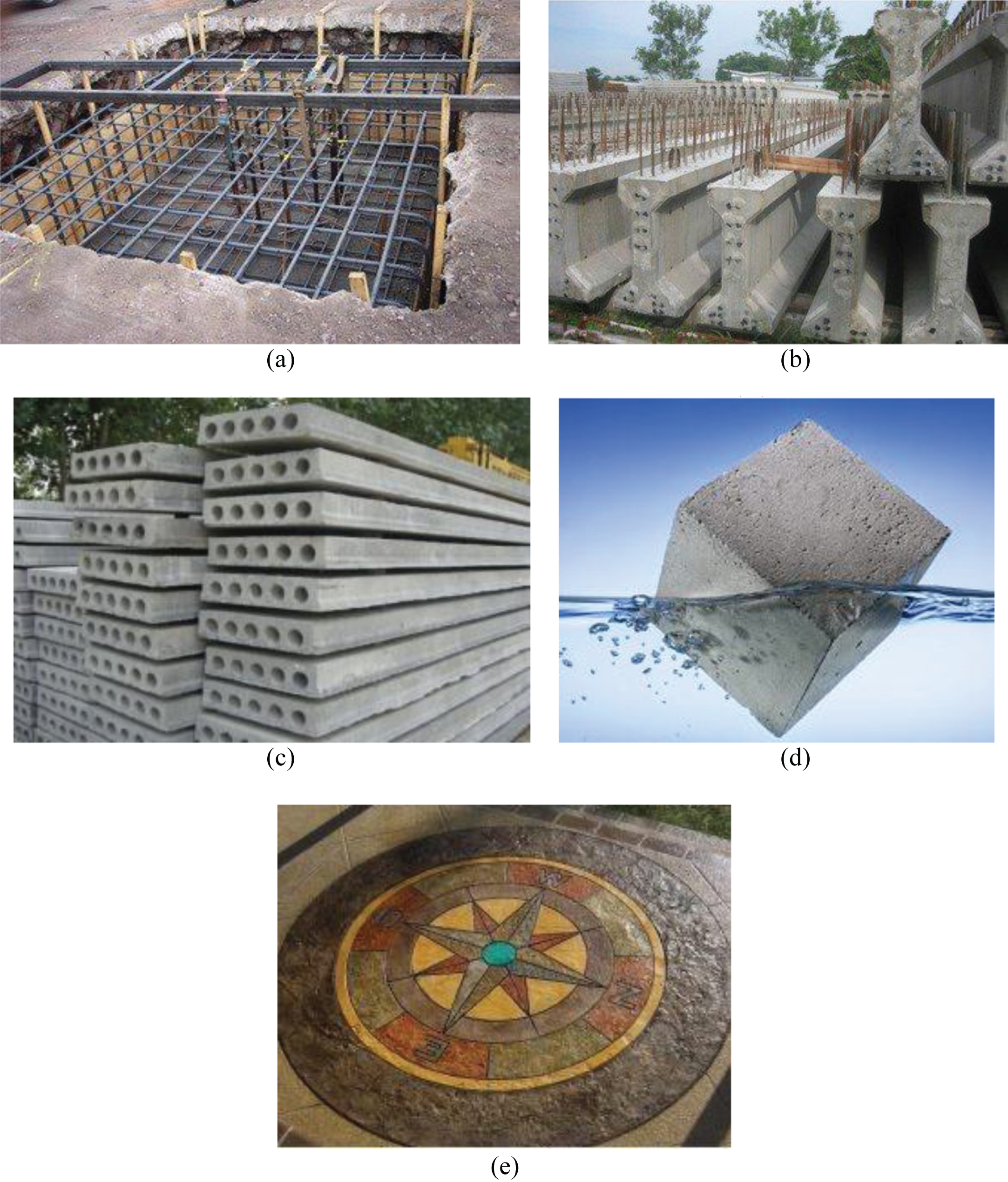
(a) Reinforced Concrete, (b) Prestressed Concrete, (c) Precast Concrete, (d) Lightweight Concrete and (e) Stamped Concrete.
HPC increase the quality and feature characteristics/buildabily of the usual concrete. Several oedinary and specific materials are utilized to produce a specific type concrete which should match the specific requirements. A specific mixing process, being positioned and healing experiences is to be required to develop and manage HPC perfectly. Moreover, expensive tests are needed to analysis and indicate the compliance with the required project requirements. Basically, HPC has been utilized in tall building, bridges, poles, agricultural applications, shotcrete repair and bridges for its properties. On an average sixteen properties are tested on HPC specimen as per the specific test method for a specific property [3]. For example, “high strength” by “ASTM 39 (AASHTO T 22)”, “high-early flexural strength” by “ASTM 78 (AASHTO T 97)”, “High-early compressive strength” by “ASTM C 39 (AASHTO T 22)”, “Abrasion resistance” by “ASTM C 944”, “Low permeability” by “ASTM C 1202 (AASHTO T 277)”, “Chloride penetration” by “AASHTO T 259 & T 260”, “High resistivity” by “ASTM G 59”, “Low absorption” by “ASTM C 642”, “Low diffusion coefficient” by “Wood, Wilson and Leek (1989) Test”, “Resistance to chemical attack” by “Expose concrete to saturated solution in wet/dry environment”, “Sulfate attack” by “ASTM C 1012”, “High modulus of elasticity” by “ASTM C 469”, “High resistance to freezing and thawing damage” by “ASTM C 666, Procedure A”, “High resistance to deicer scaling” by “ASTM C 672”, “Low shrinkage” by “ASTM C 157”, “Low creep” by “ASTM C 512 standard” is evaluated for each specimen [3]. But at the same time, all properties may not be carried out at the same specimen. As per the requirement, required properties are tested for HPC specimen.
Related with HPC strength development, numerous researches have been studied which represented that concrete strength improvement is evaluated not only by water-cement ratio, albeit it is affected through the element of other ingredients. Therefore, recorded 1030 practical data set have represented the experimental/actual adaptability of this rule within broad range and limited variations have been adumbrated. The cogency of additional material’s effect on PHC strength should be studied. This strength will vary with variation of composition of supplement material with the water-cement ratio [4]. Moreover, knowledge of composition is related with understanding of concrete nature and behavior. For this purpose, we have to optimize the mixture of concrete which is the biggest research area of HPC strength estimation. Performing the experiment in each time is costlier and time consuming so overcome this research area and reduce the experimental capital cost, GEP based HPC comprehensive strength estimation model has been developed.
GEP has the main advantage of both GA and GP techniques [5–9]. It has self optimization characteristic which is very important property for modeling of material behavior. In this domain, several ANN based model have been modeled for modeling of material behavior [4]. But, due to numerous limitations of ANN models, GEP play a heuristic analysis for HPC comprehensive strength. Moreover, this is the very first attempt to develop GEP modeling in this domain to evaluate the comprehensive strength. While, there are numerous applications of GEP in other domain [5–9].
This paper is presented into four section. Section 1 represent the back ground highlight of the study. Experimental datasets used and methdology have been represented in section 2. In methodology, proposed approach and Step-by-step procedure for development of GEP and RBF model haven explained. Section 3 explain the obtaine results and discussed in detail and conclusion of the study is represented in section 4.
Data set used
The experimental data sets of 1030 samples has been collected from publicly available resources of UCI Machine learning Reprository [4]. This data sets includes eight input variables (i.e., cement, blast furnaces slag, fly ash, water, superplasticizer, coarse aggregate, fine aggregate and age) of different composition levels. The measurement unit for 1 to 7 input variables is kg/m3 (quantitative mixture) and last attribute is number of days for testing a sample. The range variation for each attribute is represented in Table 1 and graphicaly shown in Fig. 2.

Data Sets Components Ranges.
Data sets components ranges
Several number of concrete specimen from above analysis were computed. During the calculations, some of them were deleted due to special curing scenario and larger size of aggregation. Approximate 1030 concrete specimen were experimentaly designed under normal conditions for evaluation purposes, which is represented by an input vector Z. This input vrctor Z has one output value concrete compresive strength-CCS) corresponding to each sample, was divided into two groups: traing (700 samples) and testing (330samples) group. The train and test datasets are not included to each other during the training phase. The statistical parameters for each variables of both training and testing dataset have been evaluated and frequency based histogram representation has been represented below in Fig. 3.
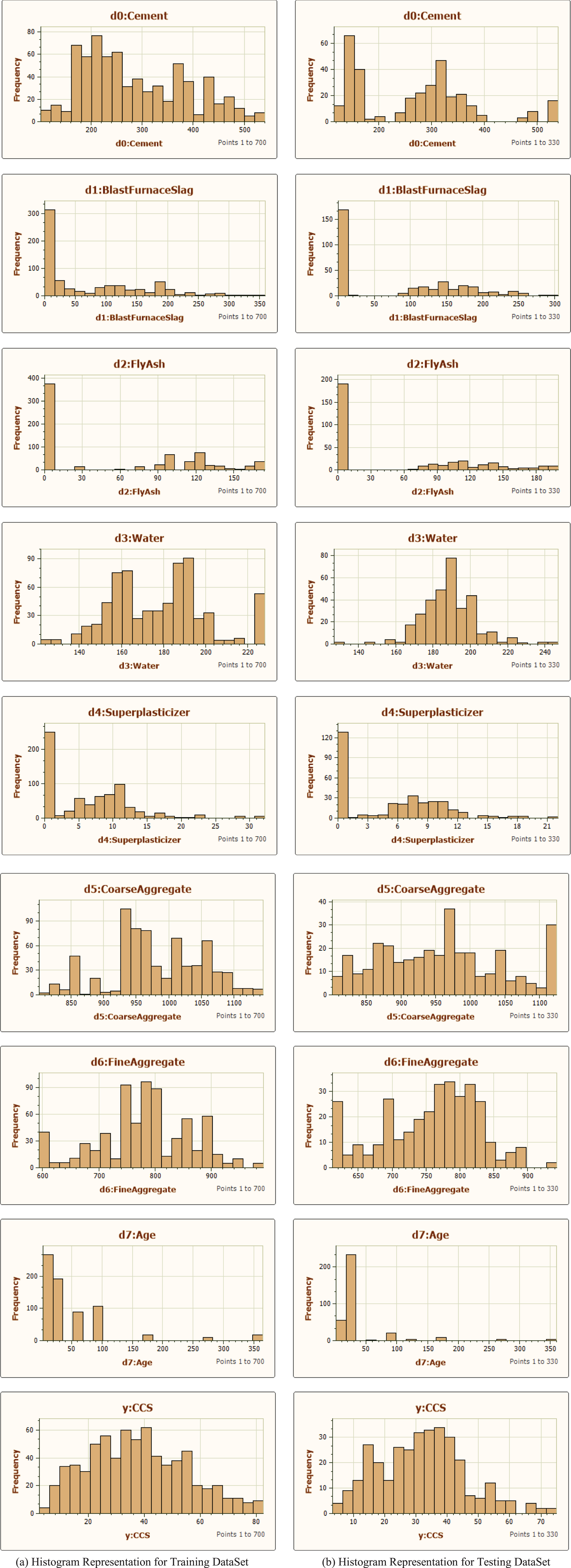
Histogram representation for training and testing data set.
After preprocessing the both training and testing data, the statistical analysis is given below for each variables in Table 2:
Statistical anaysis for training and testing data set
d1:BlastFur = BlastFurnanceSlag; d4:Superp = Superplasticizer; d5:CoarseAg = CoarseAggregate; d6:FineAg = FineAggregate; STD = standard Deviation.
Proposed approach for the prediction of HPCCS is shown in Fig. 4, which shows the step-wise-step procedure for the prediction. The selection of trained model is depends upon the minimal value of mean squared error. When training phase is performed with desired prediction accuracy, testing is done. The testing data for testing phase is totally separately than training data.

Proposed Algorithm.
The prediction accuracy of HPCCS is depends on the number of input variables. It will vary with variation of input variables. So selection of number of input variable and implementation of new approach is a major research gap in this area. To bridge this gap, Gene Expression Programming (GEP) based model for selecting most relevant input variable and prediction of HPCCS is proposed and presented in subsequence section. The big reason for choosing the GEP based model in this problem is that GEP select the variables as well as predict the target value also. So, both selection and prediction may perform by using GEP. Other big reason for opting the GEP is that it has both advantages of Genetic Algorithm (GA) and Genetic Programming (GP). Therefore, we do not require any other optimization technique for optimizing the parameters of GEP.
Entities are utilized as populations in GEP identical to GP and GA. These entities are known as parse tree. Properties of parse trees are nonlinear with distinct size and shape and are adopted as per its evaluated fitness value. The fitness value of a program is depends upon its crossover, mutation and rotation. The computation of fitness value (z
k
) of a program (k) is represented by Equations (2) and (3) [21]:
Where x = selection range, ℓ(p,i)= returned value by the individual chromosome (p) for fitness case (i) (from N fitness cases), and s i = target value for fitness case i. Figure 5 represented the expression tree formation from a developed gene of GEP model.

Expression Tree (ET) representation of a Gene.
Developed genes include tail & head. For each model, length of head (h) was provided by the user whereas length of tail (T) is computed by using Equation (4) [21]:
The arrangement of structural and functional part of genes and its representation in expression trees shows the development of valid programs. Figure 6 represents the complete working procedure of GEP model in detail.

GEP algorithm [7].
The utilization of RBF is function approximation, classification, time series prediction which is formulated first in 1988 by two researchers (Lowe and Broomhead) from Royal Signal and Radar Establishment (RSRE), Ministry of Defence (MoD), United Kingdom. The RBF network generally utilized for activation function in ANN and output is linear combination of RB functions of inputs and neuron’s parameters. The RBF network is utilized for time series prediction, classification, function approximation and controlling the system. The mathematical architect of RBF NN is given below:
Where, N = no. of hidden layer neuron, c
k
= center vector of kth neuron, w
k
= weight of k
th
output linear neuron. RBF is generally used Gaussian as:
The w k , c k and β k parameters are optimized and found as per fit between out put Z (y) and data sample y.
The Equation (4) of RBF is unnormalized, which can be normalized as:
Where,
This is known as “normalized RB function” and can be utilized for CCS prediction.
GEP based HPCCS prediction
HPCCS is evaluated by using GEP approach and obtained its mathematical model is represented below with prediction accuracy of 98.72% in testing phase:
f = gep3Rt((((reallog(((d(CoarseAggregate)/d(Cement))2))*(gep3Rt(d(BlastFurnaceSlag))2))+d(Cement))2));
f1 = f+(d(Superplasticizer)-((1.0/(reallog(gep3Rt(G2C 9))))*gep3Rt(((d(Cement)/G2C6)+(d(Superplasticizer)-d(Age))))));
f2 = f1+min(gep3Rt((d(BlastFurnaceSlag)-d(Water))), ((((d(FlyAsh)+d(Superplasticizer))/2.0)-reallog(G3C 5))*min(G3C5,d(Age))));
f3 = f2+(((((d(Superplasticizer)2)+(d(FineAggregate)-d(FlyAsh)))/2.0)+gep3Rt((d(CoarseAggregate)*d(B lastFurnaceSlag))))/(d(Age)*((G4C5+G4C3)/2.0)));
where, calculated constant variables are: G2C9 = 7.13; G2C6 = 7.26; G3C5 = 6.90; G4C5 = –2.55; G4C3 = –9.11; and evaluated rank value of each input variables is: Cement = 1; BlastFurnaceSlag = 2; FlyAsh = 3; Water = 4; Superplasticizer = 5; CoarseAggregate = 6; FineAggregate = 7; Age = 8;
Representation of a GEP model’s gene is presented below:
3Rt.X2.+.*.d0.Ln.X2.X2.3Rt./.d1.d5.d0.c9.d6.d3.d1.d5.c9.d3.d0
+
–.d4.*.Inv.3Rt.Ln.+.3Rt./.–.c9.d0.c6.d4.d7.c5.d2. c5.d3.d4.c6
+
Min2.3Rt.*.–.–.Min2.d1.d3.Avg2.Ln.c5.d7.d2.d4. c5.c7.d0.d0.c5.d0.d3
+
/.+.*.Avg2.3Rt.d7.Avg2.X2.–.*.c5.c3.d4.d6.d2.d5. d1.d1.d6.d6.d2
Where, numerical Constants for
Representation of genes into an ET is shown in Fig. 7:

ET for genes of GEP model.
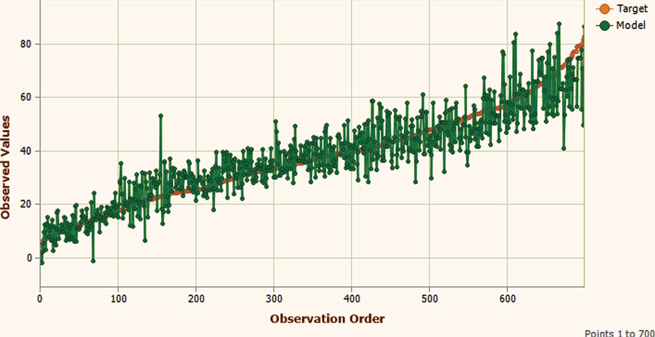
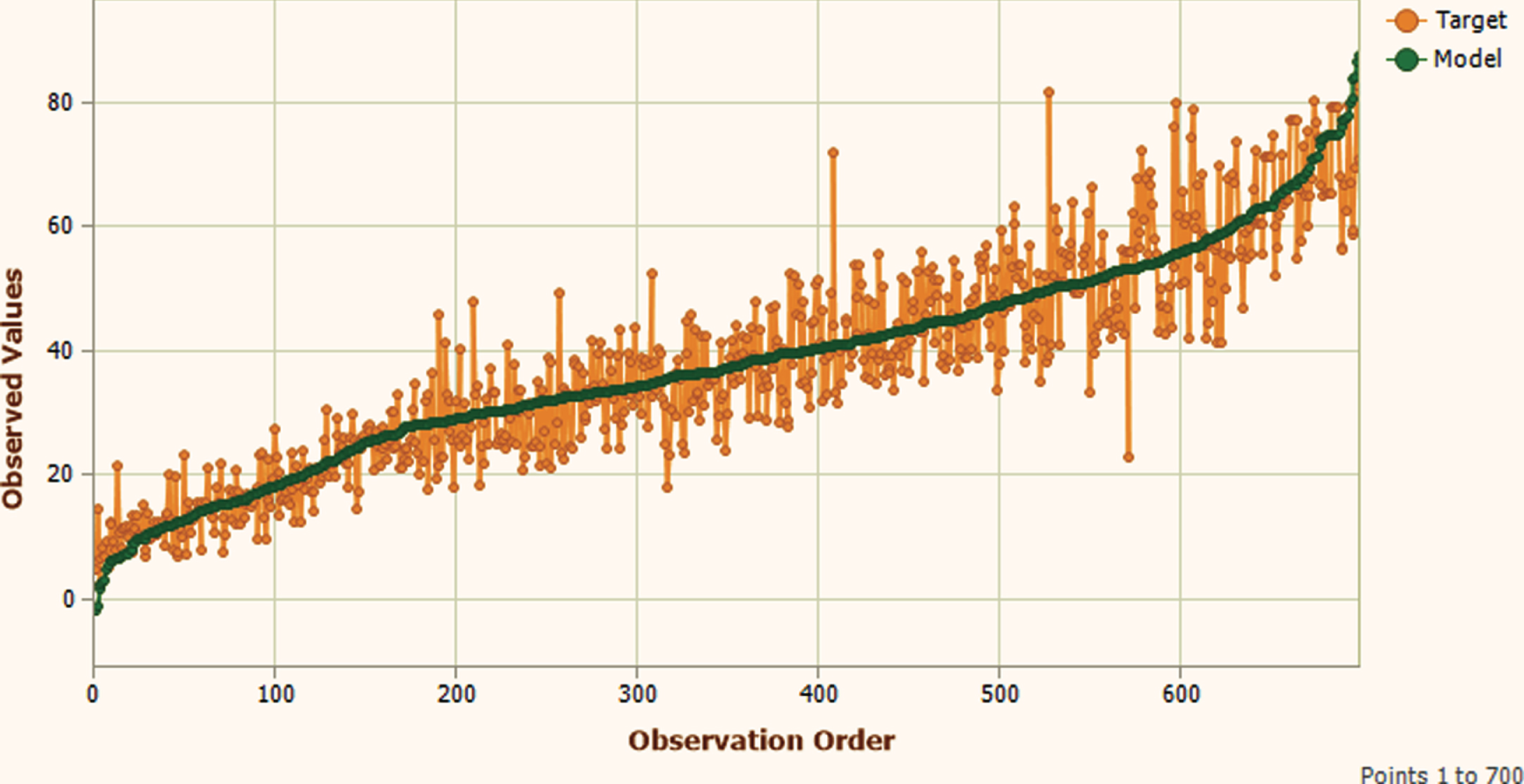
The obtained results during training and testing phase are represented in Figs. 8 to 19 respectively for further validation of the proposed GEP based model.

Training Phase Scattered plot.
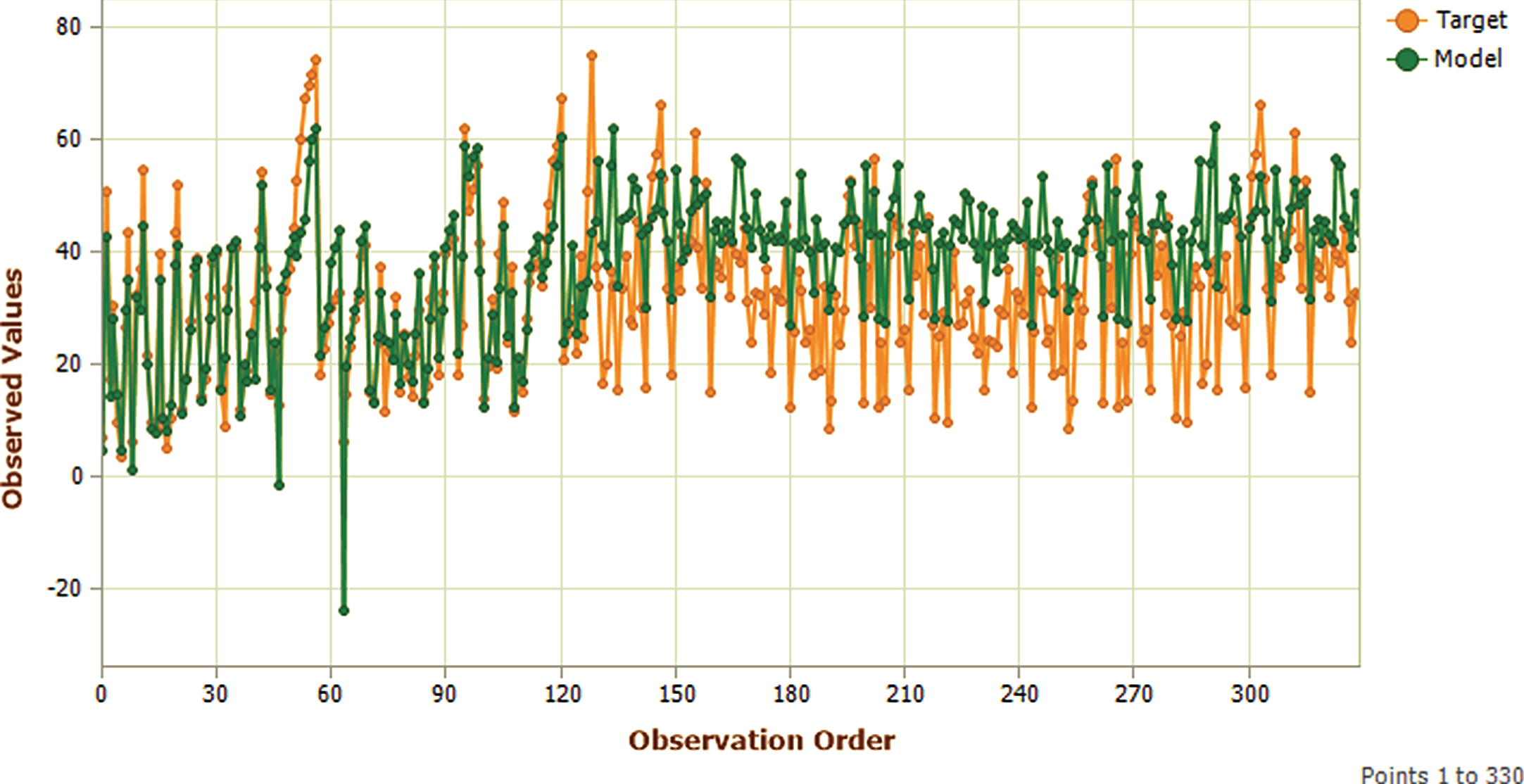
Training Phase Target shorted fitting plot.
Training Phase Model shorted fitting plot.
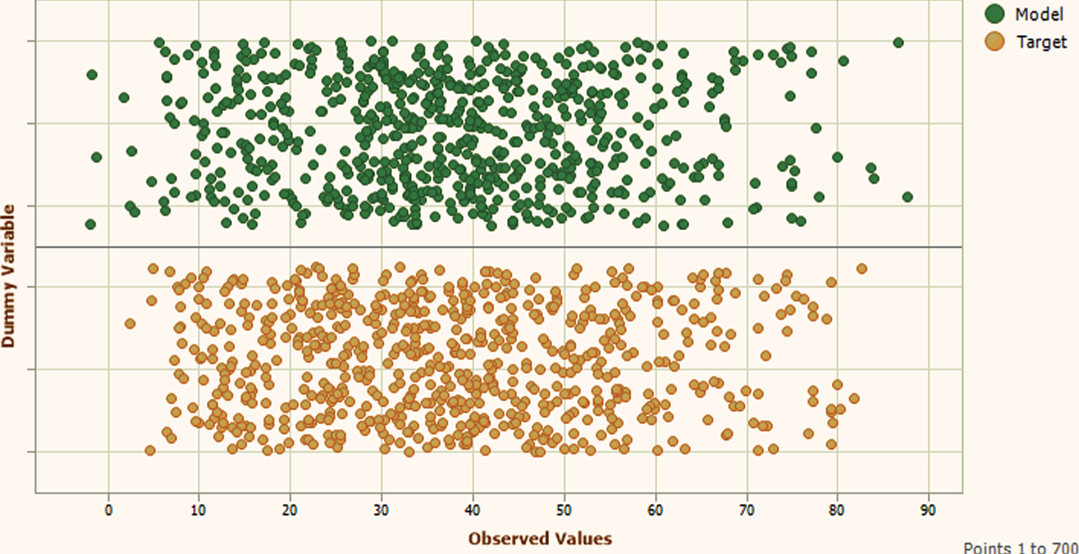
Training Phase Stacked distribution.
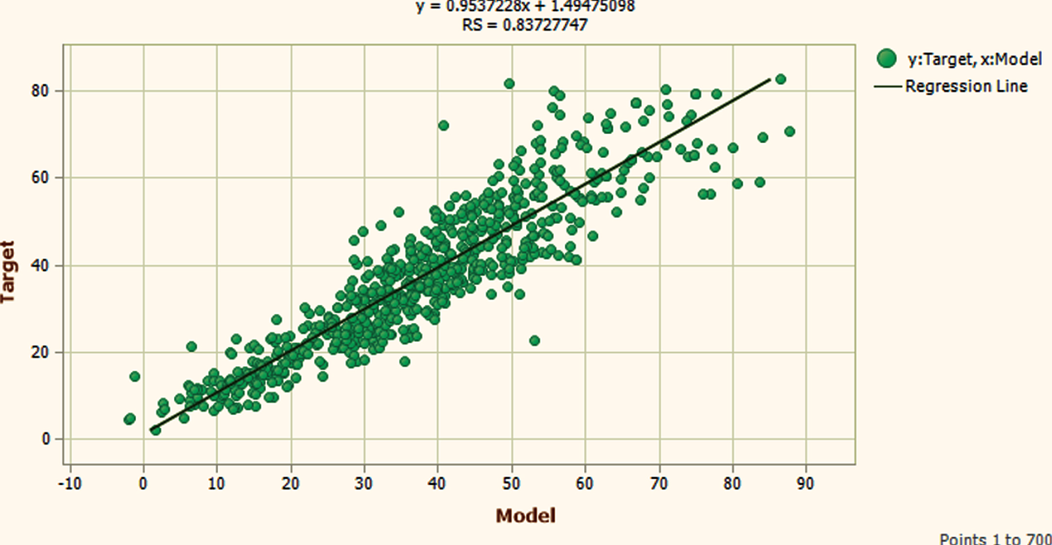
Training Phase Scatter plot.
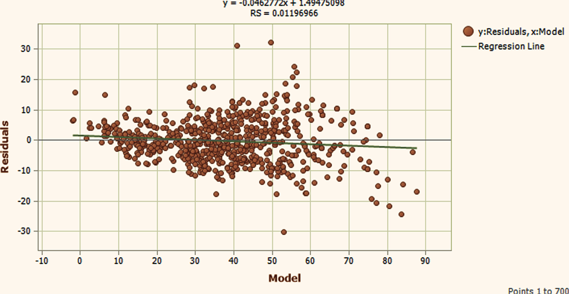
Training Phase Residual plot.
Testing Phase Scattered plot.
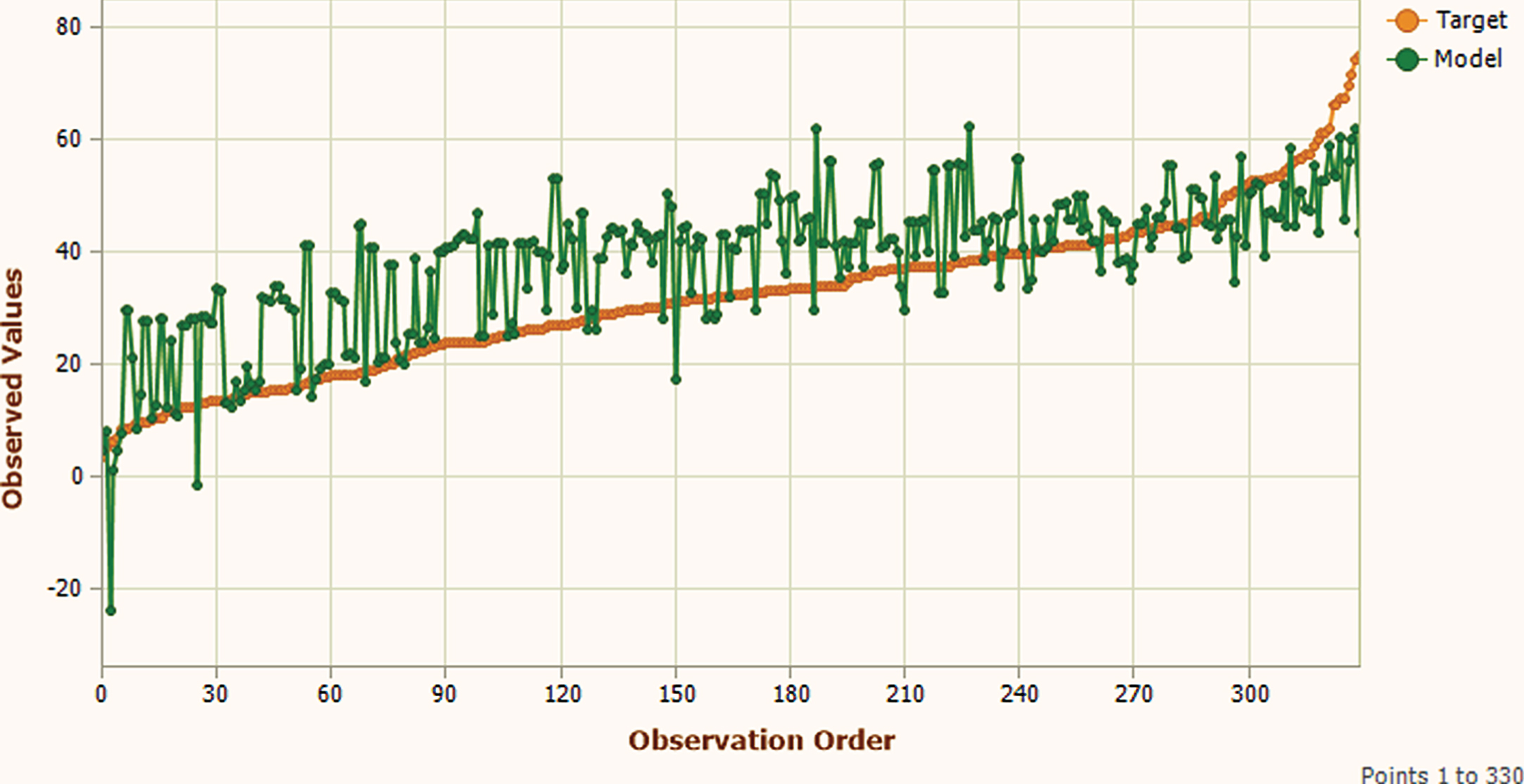
Testing Phase Target shorted fitting plot.
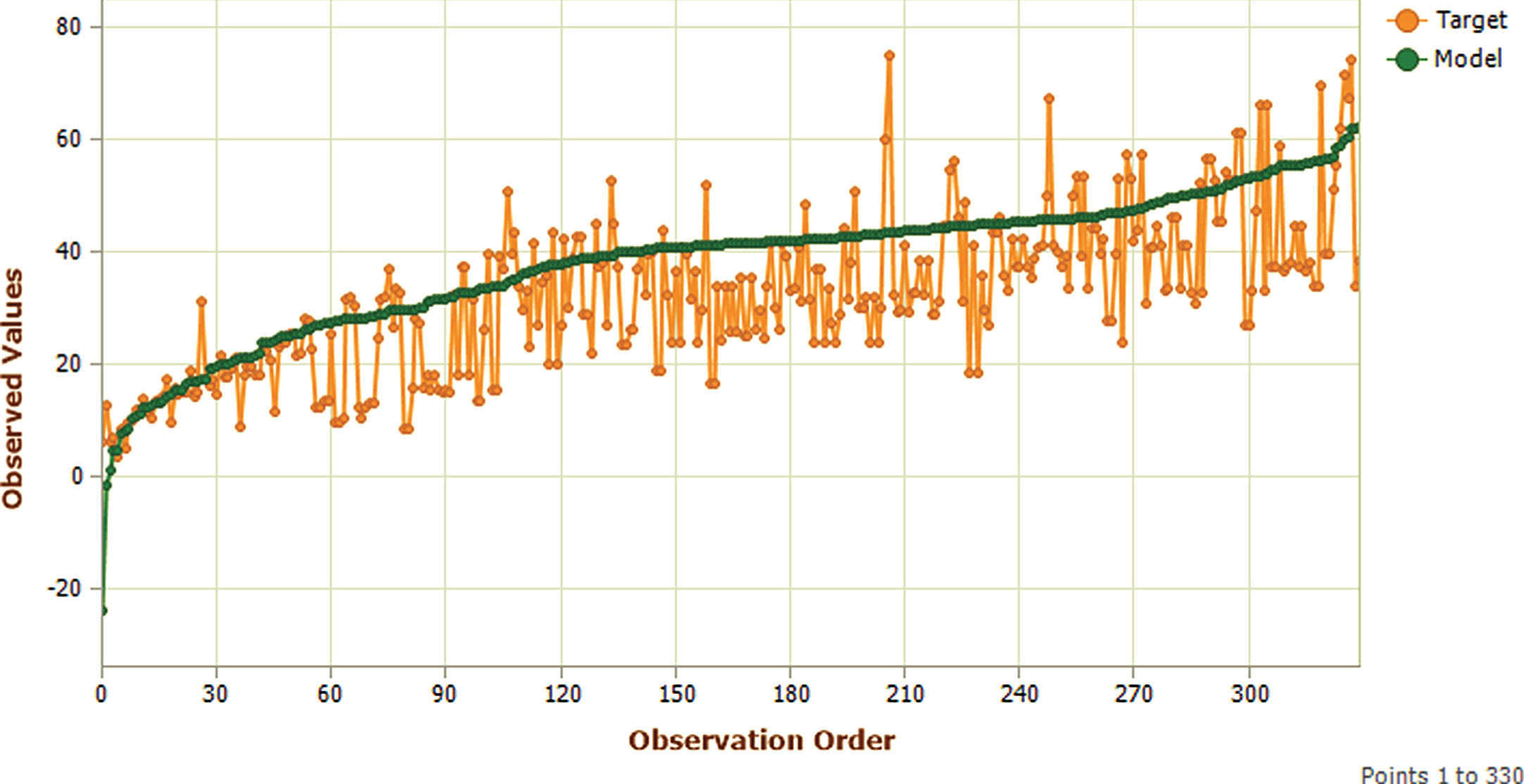
Testing Phase Model shorted fitting plot.

Testing Phase Stacked distribution.
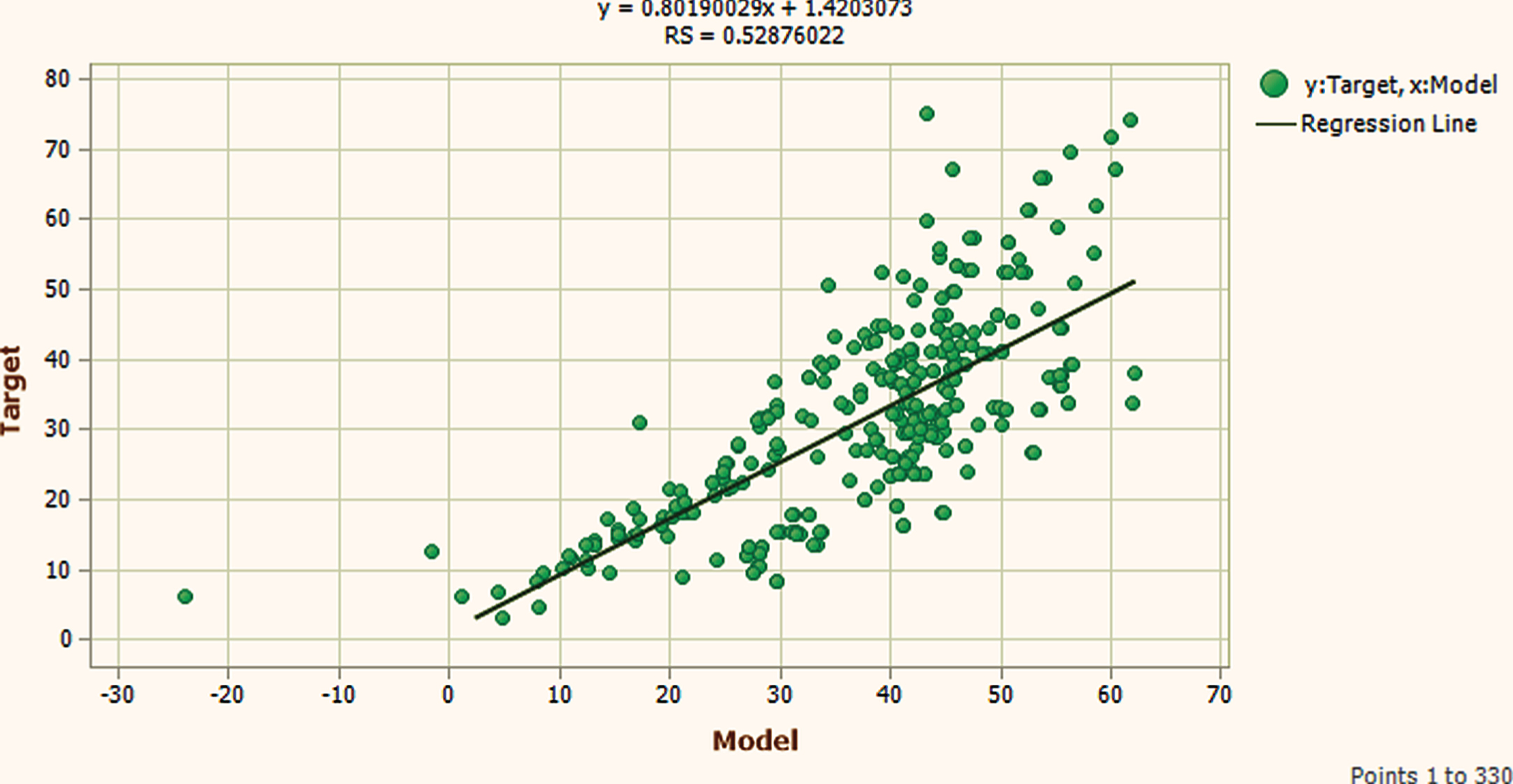
Testing Phase Scatter plot.
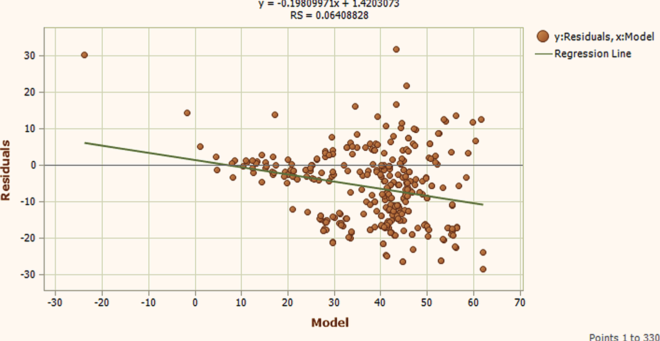
Testing Phase Residual plot.
With the help of mathemetical modelling of RBF neural network as mentioned in section 2.4, the MATLAB codes are implemented for HPCCS prediction by using radialy available 1030 experimental dataset which includes eight input neurons at input layer, one output neuron at output layer and maximum number of neurons at hidden layer is equal to the number of training data samples or may be calculated by using Equation (11) [10–16] and obtained results for training and testing phase are given in Fig. 19.
Matlab coding based regression plot for training and testing phase results are shown in Figs. 20 to 22.

Training Phase performance plot.
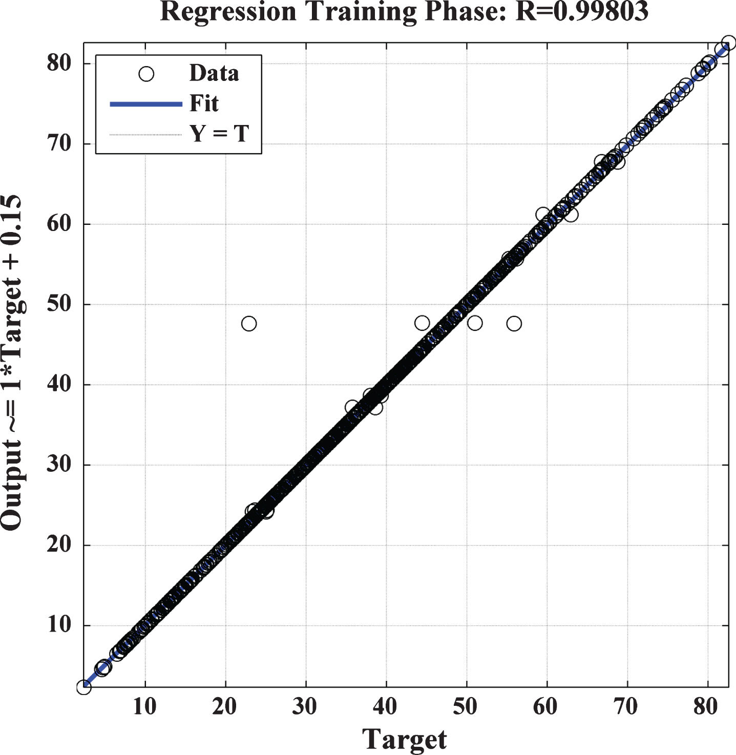
Training Phase regression plot.

Testing Phase regression plot.
For fair comparison of proposed GEP approach, RBF neural network has been designed to predict the HPCCS and the obtained results from GEP and RBF have been compared. The testing phase accuracy for GEP is 98.72% whereas 95.36% for RBF neural network, which represents advancement of GEP as compare with RBF as shown in Table 3. Some practical experimental studies have been shown in Table 4, which shows higher correlation of predicted output through GEP and RBF with respect to measured value.
Performance analysis of the GEP and RBF models
Performance analysis of the GEP and RBF models
Predicted results of 154 samples by using GEP and RBF models
In the presented paper GEP model is developed based on available 1030 data set of eight input variables for the prediction of high performance concrete compressive strength. Concrete compressive strength is predicted by using 1030 data sets. The accuracy of the proposed model is found to be 98.72% and obtained results are compared with conventional computational intelligent technique such as RBF. The HPCC prediction accuracy of RBF is 95.36% during testing phase which shows the superiority of the proposedmethod.
The future work is to implementing the proposed approach in real field.