Using radial basis function for estimating the high-performance concrete compressive strength with optimizing AVOA and SSA

Abstract

Compressive strength (CS) is concrete’s most important mechanical property, as it plays an important role in setting design criteria. Thus, an accurate and early assessment of the CS of concrete can minimize time, labor, and cost. This paper investigated the ability of the Radial Basis Function (RBF) to handle the prediction of CS. The nonlinearities raised from the novel utilized admixtures between the input variables and output CS is tried to be conducted with the RBF model. In order to make a flexible framework combination of the RBF model with the African Vulture Optimization (AVOA) and Salp Swarm Algorithm (SSA) techniques are considered. The results achieved from the RBF-AVOA model indicated good agreement between the actual and predicted values. The proposed model provides a very accurate HPC compressive strength prediction. In addition, the correlation coefficient R² is equal to (0.997), and the values of mean absolute error (MAE) (0.1917 MPa), root mean square error (RMSE) (0.937 MPa), and variance account coefficient (VAF) (99.73%) are low. The performance of the RBF-AVOA model, compared to other models, provided the desired advantage and more stable predictions. AVOA plays a key role in modeling results, improving generalization capabilities, avoiding redundant data, and decreasing uncertainty.

Keywords

High-performance concrete compressive strength african vulture optimization algorithm salp swarm algorithm radial basis function

1 Introduction

Concrete is widely utilized as a building material because of its availability, economical, and widely applicable [1]. However, its fragility is its main drawback when used in seismic zones. The main disadvantages which need to be overcome are less tensile strength and less tensile strength to tearing and spreading [2]. The scenarios as mention have resulted in a great need for concrete with critical qualities like high strength, high workability, durability, and toughness [3]. High-performance concrete (HPC) [4], High-strength concrete (HSC), and fiber-reinforced high-performance concrete composite (FRHPCC) are some sorts of concrete.

Compared to conventional concrete, they have excellent attributes [5]. HPC production requires supplemental cement-based materials such as bagasse ash, silica fume, and fly ash as a binder [6, 7]. Under typical conditions, replacing regular Portland cement with a concrete microfilter can decrease the concrete’s porosity, especially in the long term. Also, mineral additives such as bagasse ash contribute to the concrete’s brittleness [8]. Cracks typically occur over time for various reasons, containing dry shrinkage in hardened concrete and plastic shrinkage in the pre-cured state. Therefore, these cracks weaken the concrete’s water resistance and expose concrete structures to being affected by destructive substances such as chlorides, moisture, bromine, and sulfates [9]. Therefore, improving the hardened concrete’s attributes is an important concrete technology goal [10].

Over the last few decades, much attention has been paid to applying artificial neural networks (ANNs) in specifying the concrete’s compressive strength [11]. No theoretical relationship is needed between the dosage of its components required to establish the ANN model and the concrete’s compressive strength [12]. The essentials are a sufficient database for the training and testing process. With a well-trained ANN, able to enter numbers representing the dosage of concrete components like cement, water, other mixtures, and sand, ANN quickly provides the expected concrete’s compressive strength [13 –15].

ANN applications typically need to split the database into 2 sets, 1 for learning and 1 for validation. Generally, the test suite should include at least 10% of the databases. If not, ANNs tend to overload the train set, resulting in poor performance in real-world applications. ANN models have been developed to predict the concrete’s CS for 28 days. They used a database that also built an ANN model for the same application. Data has been reorganized. Fewer data are used for testing, and more data is used for training [16 –21].

Fly ash (FA) is a fine-grained material produced by burning coal to powder in the furnaces of power plants [7]. Electrostatic or mechanical precipitators collect by-products of such power generation and are widely used by engineers in the concrete industry to decrease anthropogenic CO2 emissions [22]. FA is important in the concrete matrix, containing microstructural performance, workability, and strength. FA is usually considered a collection of particles that affect the performance of concrete as a combined result of the several particles’ effects [23]. Sink beads are a hydro-cyclone-separated fly ash component that absorbs about 40% of FA per unit weight. The chemical and physical attributes of submerged spheres, like particle size, density, compressibility above 700 MPa, and pozzolanic activity, differ from fly ash and significantly impact HPC performance in real-world engineering applications. Nevertheless, little literature is related to subsidence pearls, especially subsidence pearls as an alternative cement component to HPC cement [24].

Silica fume (SF) has two functions: concrete filler and pozzolan. Increasing the silica fume content reduces the concrete’s workability but improves short-term mechanical details like 28-day CS [25]. Although the publication details that the silica fume’s usage in concrete significantly improves the concrete’s mechanical properties, researchers have not reached a firm conclusion on the optimal proportion of silica fume alternatives [26]. Some researchers have shown varying degrees of substitution as optimal for achieving maximum concrete strength, and others have studied characteristic parameters affecting the concrete’s compressive strength. For the past two decades, these parameters have included cement-based materials, FA and SF in particular [27 –29].

Radial basis function (RBF) neural networks have excellent pattern variety and function-matching capabilities. This is a three-tier forward network. It contains a three-tiered network [30]. The first layer is the input layer, and the number of nodes corresponds to the input dimension. The second layer is the hidden layer; the nodes’ number depends on the issue’s complexity. The third layer is the transport layer. The nodes’ number outside the layer corresponds to the output data’s dimension [31]. RBF neural networks’ different layers have different functions. The hidden layer is non-linear. The RBF function is utilized as a basis function to transform an input vector space into a hidden layer space, linearizing the original linear inseparable issue and linearizing the output layer.

The present study tries to define a flexible model which can conduct with the complex nonlinearity between input variables and output. This complexity multiplies considering the cementitious admixtures. To handle this complex problem, a hybrid framework capable of adapting to different forms of mixed design and corresponding various nonlinearity is introduced. The radial base function facilitates the main task of modeling, and the adaption task is carried out by the novel optimization algorithms, namely the African Vulture Optimization and Salp Swarm Algorithm. The results of the novel hybrid model and their performance in the prediction of compressive strength are justified to find out a model that meets the desires in prediction with acceptable accuracy.

2 Materials and methodology

2.1 Data gathering

This study evaluated the final dataset of 170 conventional Portland cement samples, including various additives and cured under normal conditions [32, 33].

The dataset contains varying percentages of class F fly ash, silica fume, and superplasticizer. The class F fly ash, classified as ASTM class F, is in powdered form and used as a substitute for cement. It replaces a range of 0 to 55% of the binder materials in different mix designs, with a maximum utilization of 275 kg/m3. The condensed silica fume (SF) is also used as a replacement for binder, ranging from 0 to 5%. The dataset is divided into three parts based on the water-to-cement ratio (0.3, 0.4, 0.5). The mix designs incorporate ASTM type 1 Portland cement.

Table 2 shows eight items: cement (C), fly ash (Fa), Micro silica (MS), water (W), total aggregate (Ta), coarse aggregate (Ca), and Superplasticizer (SP), the input parameters. Moreover, the ratio of input variables related to cement content was presented. Also, a parallel of the data is shown in Fig. 1. Unexpected accuracy of input variables like fly ash and Micro silica was indicated. Here, the maximum (Max), minimum (Min), average (Ave), and standard deviation (St.dev) of CS are 107.8, 24, 64.03, and 15.35 MPa, respectively. Except for CS, the final output, the remaining variables are expressed in (kg/m3). Table 1 and Fig. 1 show that the CS resolution depends on not only the seven variables’ usage but also a complex procedure to determine the strength of concrete. This problematizes the strategy of predicting this type of data. These ratios mean that the effects of total aggregate, fly ash, and silica fume on CS are equal. However, the coefficient of variation and ratio input variables should affect the sensitivity of the design model. In addition, many components and ratios complicate CS calculations. The data was split into 70% and 30% as learning and validation datasets.

Table 1
The variables contained in the dataset and their statistical property

Variables Unit Statistical properties

Max Min Ave St.dev

Compressive strength (CS) (MPa) 107.8 24 64.03232 15.3551

Binder (B) (kg/m³) 500 394 418.381 40.137

Fly ash (FA) (kg/m³) 275 0 101.08 66

Micro Silica (MS) (kg/m³) 43.3 0 21.843 17.88

Superplasticizer (SP) (kg/m³) 13 0 4.472 3.094

Coarse aggregate (CA) (kg/m³) 1157 1086 1133.571 24.405

Total aggregate (TA) (kg/m³) 186 1668 1805.786 63.249

Water (W) (kg/m³) 205 118.2 165.64 28.703

Age day 180 28 68.57 49.99

Variables	Unit	Statistical properties
Compressive strength (CS)	(MPa)	107.8	24	64.03232	15.3551
Binder (B)	(kg/m³)	500	394	418.381	40.137
Fly ash (FA)	(kg/m³)	275	0	101.08	66
Micro Silica (MS)	(kg/m³)	43.3	0	21.843	17.88
Superplasticizer (SP)	(kg/m³)	13	0	4.472	3.094
Coarse aggregate (CA)	(kg/m³)	1157	1086	1133.571	24.405
Total aggregate (TA)	(kg/m³)	186	1668	1805.786	63.249
Water (W)	(kg/m³)	205	118.2	165.64	28.703
Age	day	180	28	68.57	49.99

Table 2

Developed assessment results of models by evaluators

Hybrid Models	Sections	Evaluators
		R²	RMSE	MAE	VAF
RBF-AVOA	Learning	0.9869	1.7655	0.7511	98.6691
	Validation	0.9974	0.9191	0.1917	99.7395
RBF-SSA	Learning	0.9851	1.7883	0.884	98.44
	Validation	0.994	1.3127	0.4942	99.3968

Fig. 1

The parallel plot of HPC ingredients and related compressive strength.

Fig. 2

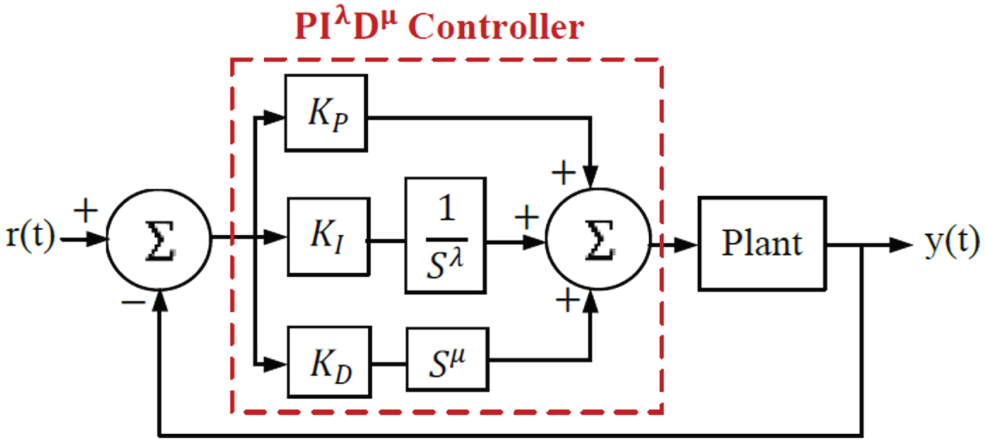
Controller structure of PD^μ-I^λ [40].

Fig. 3

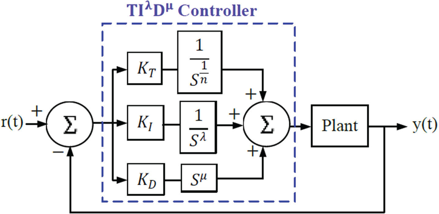
Controller structure of TI^λD^μ [40].

Fig. 4

Controller structure of PD^μ-I^λT [40].

2.2 African vulture optimization algorithm (AVOA)

The African Vulture optimization algorithm (AVOA) was utilized to select the optimal parameters for PD_μ-I^λT control. This algorithm is a meta-simulation for discrete and continuous optimizations and various explored issues. The AVOA method influenced the African vultures’ manner through feeding and navigation. AVO algorithm is split into several stages. Each stage of the algorithm formula below is the algorithm’s definition.

2.2.1 Primary stage

The first resident is formed. Then the effectiveness of the complete solution is calculated. Candidate solutions can be split into two groups. The best solution is determined for each group. Equation (1) is also employed with other options to achieve an impressive solution for groups one and two. It is the vulture that best F(i) explains. At each fitness iteration, the total population is recomputed.

$F (i) = {\begin{matrix} {Bestvulture}_{i} {ifT}_{i} = A_{1} \\ {Bestvulture}_{2} if T_{i} = A_{2} \end{matrix}$ (1)

The A₁andA₂ are the sum of both parameters equal to 1 and is in the range [0,1]. For each group, according to the A₁andA₂ ’s values, the remaining vultures assemble in one of the solutions sufficient. Depending on the group:

$T_{i} = \frac{R_{i}}{\sum_{i = 1}^{n} R_{i}}$ (2)

The P exhibits vulture is filled. The value of S is defined by Equation (3):

$R = (2 \times {rand}_{1} + 1) \times y \times (1 - \frac{{rep}_{i}}{maxrep}) + u$ (3)

Equation (4) specified u:

$\begin{matrix} u = v \times (\sin^{n} (\frac{π}{2} \times \frac{{rep}_{i}}{maxrep}) \\ + \cos (\cos^{n} (\frac{π}{2} \times \frac{{rep}_{i}}{maxrep}) - 1) \end{matrix}$ (4)

The rep_i indicates the iterations’ current number. maxrep determined an integer iteration’s maximum. Random numbers in the range [1,1], [2,2], and [0,1], respectively, for rand, y, and v. Before the optimization operation, n Constant coefficients were adjusted.

2.2.2 Searching stage

The AVOA searching phase is currently under consideration. Two formula-based methods (5). Also, one must set the F1 parameter in the range [0,1] and select one of the two methods before exploring. The following formula can be expressed at this phase in the following:

$\begin{matrix} T (i + 1) \\ = {\begin{matrix} F (i) - B (i) \times R if F_{1} ⩾ {rand}_{f 1} \\ F (i) - R + {rand}_{2} ((ud - ld) \times {rand}_{3} + ld) \end{matrix} \end{matrix}$ (5)

$B (i) = | Y \times T (i) - T (i) |$ (6)

The T (i + 1) displays the vector of the vulture’s status at the current iteration. rand_f1andrand₂ generated between 0 and 1 and defined the random numbers. Y indicates a non-systematic motion enhancement coefficient vector. The value of Y can be calculated as X = 2×rand and changes during the iteration. udandld show the upper and lower limits of the variable. rand₃ is used to increase the factor of randomness.

2.2.3 Utilization stage

This stage tests the AVOA’s effectiveness. Furthermore, this phase is divided into two stages, each utilizing two different methods. To choose between two methods, Stage one and Stage two, the parameters F₂ and F₃ are used to determine, respectively. The values F₂ and F₃ are assigned before performing the search,

2.2.4 Primary utilization step

If the |R| ⩾ 0.5, AVOA penetrates the first Utilization step. In the range [0,1], this step begins by developing a random number called rand_R2. This step with different methods is given by equation (7). In addition, vultures often make regular spiral flights. Formula (9) and (7) are employed to model rotary flight.

$\begin{matrix} T (i + 1) \\ = {\begin{matrix} B (i) \times (R + {rand}_{4}) - a (t) if S_{2} ⩾ {rand}_{R 2} \\ T (i) - (R_{1} + R_{2}) if S_{2} < {rand}_{R 2} \end{matrix} \end{matrix}$ (7)

$a (t) = T (i) - F (i)$ (8) $\begin{matrix} R_{1} = F (i) \times (\frac{{rand}_{5} \times T (i)}{2 π}) \times cos (T (i)) \end{matrix}$

$R 2 = F (i) \times (\frac{{rand}_{6} \times T (i)}{2 π}) \times sin (T (i))$ (9) here rand₄, rand₅ and rand₆ have random values from 0 to 1; a (t) indicates the distance between the vulture and one of the best vultures of the two groups.

2.2.5 Secondary utilization step

AVOA initiates the second step of Utilization when the value of |R| < 0.5 Furthermore, at the beginning of this step, a random number in the range [0,1] described by rand_F3 is developed. This step with different methods is given by equation (12).

Due to food competition, multiple vultures may move toward the same food source. Formulations (22) and (23) can be used to formulate this movement.

On the other hand, other vultures become aggressive when looking for food. They all move toward the vulture’s head in different positions. An expression to simulate these settings uses equation (24).

Here, BestVulture₁ (i) andBestVulture₂ (i) are the best vultures of each of the two groups. b shows the dimensions of the problem. Furthermore, y and w are random numbers, their values vary from 0 to 1, and α represents several fixed.

$\begin{matrix} T (i + 1) \\ = {\begin{matrix} \frac{(U_{1} + U_{2})}{2} (10) if T_{a} ⩾ {rand}_{F 3} \\ P (i) - | b (t) | \times \times ER (b) (11) if T_{a} < {rand}_{F 3} \end{matrix} \end{matrix}$ (12)

$\begin{matrix} U_{1} = & {BestVulture}_{1} (i) \\ - \frac{{BestVulture}_{1} (i) \times P (i)}{{BestVulture}_{1} (i) \times P {(i)}^{2}} \times R \end{matrix}$ (13) $\begin{matrix} U_{1} = & {BestVulture}_{2} (i) \\ - \frac{{BestVulture}_{2} (i) \times R (i)}{{BestVulture}_{2} (i) \times R {(i)}^{2}} \times R \end{matrix}$

$ET (a) = 0.01 \times \frac{y \times δ}{{| w |}^{1 / α}}$ (14)

$δ = (\frac{τ (1 + α) \times sin (\frac{π α}{2})}{τ (1 + 2 α) \times α \times 2 \times \frac{(α - 1)}{2}})$ (15)

2.3 Salp swarm algorithm (SSA)

Salp Swarm Algorithm (SSA) [34] is a new optimization method for solving various optimization issues. It stimulates the salp’s manner in the wild; Salp is a barrel-shaped enveloped plankton and a member of the Salp family. Moreover, their tissues are similar to jellyfish, and their motion, demeanour, and body weight have high water content. Pumping water through the gelled body changes its location, and its motion is by contraction [35, 36]. Marine salp has a herding habit called the salp chain. This manner can help promote motion and feed through rapid changes in harmony [37, 38]. According to this behavior, the algorithm has modeled the Salp series in a mathematical format and tested it with an optimization issue [39].

SSA begins by dividing the population into two groups: leaders and followers. The other salps are called the following, and the previous salp in the sequence is called the leader. The position of the salp is specified in n dimensions, representing the problem’s search space, where n defines the variable in question. These salps look for food sources that indicate the herd’s destination. Use the following formula to perform this action on the Salp leader since the location needs to be updated frequently:

$y_{j}^{1} = {\begin{matrix} P_{j} + b_{1} (({ud}_{j} - {ld}_{j}) b_{2} + {ld}_{j}) b_{3} ⩽ 0 \\ P_{j} + b_{1} (({ud}_{j} - {ld}_{j}) b_{2} - {ld}_{j}) b_{3} > 0 \end{matrix}$ (16)

Here $y_{j}^{1}$ is the leader’s position in the j^th dimension, the food source in that dimension is P_j, and the lower and upper bounds are ldandud_j, respectively. b₂ and b₃ are randomly generated in the range [0,1] to explore space. The parameter b₁ is also a very significant factor in this algorithm because it serves to balance between the search stage and the utilization stage and is computed in the following:

$n_{1} = 2 e^{- {(\frac{4 l}{l_{\max}})}^{2}}$ (17)

Here l_max and l show the maximum number of iterations and the current repetition, respectively. After updating the position of leader, SSA begins updating the position of follower utilizing the following formula:

$y_{j}^{i} = \frac{1}{2} (y_{j}^{i} + y_{j}^{i - 1})$ (18)

$y_{j}^{i}$ is the i^th position of the follower in the j^th dimension, and (i) is bigger than 1.

2.4 Radial basis function (RBF)

Due to the radial basis function neural network (RBFNN) can approximate difficult non-linear terrain from input and output data employing a simple topology method, it has become very popular these days. The RBFNN is a domain approximation network that simulates the neural network system of the adaptive human brain region and mutual envelope-receiving regions. A feedforward neural network with hidden layers and structure-matching specification functions has three layers, and the output layer is linear weight independent. Compared with BP neural network, there is no issue of slow region reduction or isotropic, and the speed of knowledge is fast, so it is widely employed in function approximation, pattern diagnosis, image processing, and non-linear time series prediction.

An RBF neural network’s topology system contains input, hidden, and output layers. In addition, sending the details without any processing is the responsibility of the input layer. The hidden layer helps to generate a local response to the input signal. The output layer employs a linear method to weigh the hidden layer’s output linearly. A schematic diagram of the system is illustrated in Fig. 5. This terrain from the input layer to the output layer is non-linear, but the terrain from the hidden layer to the output layer is a linear network system that evades minimal issues in local systems and improves learning speed.

Fig. 5

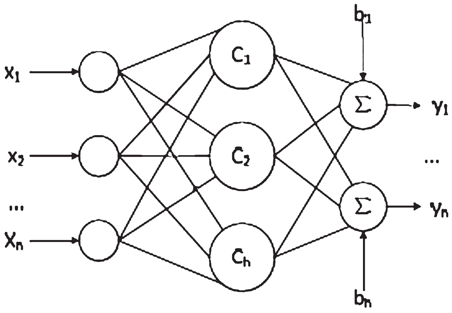
Structure of RBFNN [41].

Where the hidden layer’s processing activity, which is the radial process δj, can be defined in the following:

$δ j (Y) = exp (- \frac{∥ x - {cj}^{2} ∥}{2 ρ_{j}^{2}})$ (19)j = 1, 2, ... , n

In the equation, Y is the input detail, and the center of the j^th radial basis function is c_j, and the basis function variance is ρ_j, and the number of hidden layer neurons is n.

The output layer is in the following:

$x_{m} = \sum_{j = 1}^{n} w_{jm} δ j (Y) + b_{j}$ (20)m = 1,2, ... , n

2.5 Evaluation criteria

Various statistical criteria were applied to evaluate the validity of the assumed model RBF-AVOA and RBF-SSA against the reference model. Correlation coefficient (R²), root mean square error (RMSE), mean absolute error (MAE), and variance account factor (VAF).

$R^{2} = {(\frac{\sum_{i = 1}^{n} (p_{i} - \bar{p}) (t_{i} - \bar{t})}{\sqrt{[\sum_{i = 1}^{n} {(p_{i} - \bar{t})}^{2}] [\sum_{i = 1}^{n} {(t_{i} - \bar{t})}^{2}]}})}^{2}$ (21)

$RMSE = \sqrt{\frac{1}{n} \sum_{i = 1}^{n} {(t_{i} - p_{i})}^{2}}$ (22)

$MAE) = \frac{1}{n} \sum_{i = 1}^{n} | t_{i} - p_{i} |$ (23)

$VAF = (1 - \frac{var (t_{n} - y_{n})}{var (t_{n})}) \times 100$ (24)

The samples’ number is defined by n. The predicted and measured data are described by p and t, and $\bar{p}$ and $\bar{t}$ represent the average of the predicted and actual datasets, respectively. For more detailed analysis, use graphs to explain the prediction accuracy of each model better and help obtain the rapid and summary information that is very important in the evaluation phase.

3 Results and discussion

The Radial Basis Function (RBF) was employed as a model to obtain the concrete’s compressive strength by combining the two mentioned optimizers. Accordingly, the hybrid models’ frameworks are RBF-SSA and RBF-AVOA. The samples are divided into two sections, including learning and validation, where 70% of the samples belong to the learning, and 30% are related to the validation section. In addition, the performance of the hybrid models has been evaluated via the evaluation criteria introduced in section 2.5.

Table 2 shows four evaluators, including R², RMSE, MAE, and VAF, for the two integrated models RBF-AVOA and RBF-SSA in the learning and validation sections. The maximum R² and VAF are the best modes for these evaluators, and the minimum RMSE and MAE are the ideal model modes. As shown in the table, the maximum value of R² equals 0.9974, which belongs to the RBF-AVOA model in the validation section. However, the minimum value is obtained by the RBF-SSA model in the learning section equal to 0.9851. In addition, like R², the RBF-AVOA model showed better performance in RMSE. In this regard, the corresponding RMSE value for RBF-AVOA equals 0.9191 in the validation section, and the weakest performance in terms of RMSE value is for the learning section obtained by the RBF-SSA model, equal to 0.9851. The MAE evaluator’s minimum value equals 0.1917, which belongs to the RBF-AVOA model in the validation section, and the maximum value equals 0.884, which belongs to the RBF-SSA model in the learning section.

Moreover, the VAF metric, which should be at the highest level in the combined RBF-AVOA model, has a numerical validation portion equal to 99.7395, and the minimum value for this metric is 98.44 in the training portion of the RBF-SSA model.

The output of the present study is compared with some recently published articles which developed models to predict the compressive strength of HPC concrete. The comparison is accomplished by considering the R² values. According to Table 3, many models are considered to have comprehensive comparisons. However, the present study occupied the first place regarding model performance and accuracies.

Table 3
Comparison of present study performance with recent studies

Work ID Employed Model R²

Present work RBF-AVOA 0.9974

Xiaoxuan Hu [42] GWO-SVR 0.9706

Mosavi et al. [43] GEO 08224

Gandomi et al. [44] Multi-GGP 0.8224

Asteris et al. [45] GPR 0.9877

Nguyen et al. [46] SEM 0.84

Dao et al. [47] GPR 0.888

Nguyen et al. [48] XGBoost 0.944

Zhu et al. [49] AOA-SVR 0.9874

Work ID	Employed Model	R²
Present work	RBF-AVOA	0.9974
Xiaoxuan Hu [42]	GWO-SVR	0.9706
Mosavi et al. [43]	GEO	08224
Gandomi et al. [44]	Multi-GGP	0.8224
Asteris et al. [45]	GPR	0.9877
Nguyen et al. [46]	SEM	0.84
Dao et al. [47]	GPR	0.888
Nguyen et al. [48]	XGBoost	0.944
Zhu et al. [49]	AOA-SVR	0.9874

Figure 6 shows a scattered representation of the correlation between the predicted and measured values of CS in the two integrated models, RBF-AVOA and RBF-SSA. These forms consist of five characteristics, namely:

Learning and validation are specified as points in each section.

Linear Fit, showing the intermediate status of all samples related to each section with a red line.

The centerline with coordinates Y = X is drawn as dashes between the samples.

The support line is the upper line with coordinates equal to Y = 1.1X.

The bottom line is also a support line with coordinates Y = 0.9X.

Fig. 6

The scatter presentation of correlation between measured and predicted values of compressive strength.

This section’s points should lie between the two support lines and near the centerline. Furthermore, if the points leave the lower (Y = 0.9X) and upper (Y = 1.1X) lines, they are considered underestimated and overestimated, respectively. Part (a) deals with the combined RBF-AVOA model, and as can be seen, only one point is above the high support line, and the rest are near the midline, which is the most appropriate state. On the other hand, in part (b) for the RBF-SSA model, one of the samples is underestimated. Both hybrid models show good performance, but the RBF-AVOA model shows higher density around the bisector line, which means better performance.

Figure 7 shows the error rate plot for the developed model. The right and left sides of this figure belong to the hybrid models RBF-SSA and RBF-AVOA, respectively, and each model includes learning and validation phases. The variation of error percentages in this graph placed between 10 and –10 percent for the RBF-AVOA model in the learning phase, although a sample in this section exceeded this domain and recorded an error of –10.1%. The same treatment is also calculated for RBF-AVOA in the validation part which, in a sample, the reported error is higher than the mentioned domain, about 2.93%. Fluctuations outside these numbers indicate an excessive error.

Fig. 7

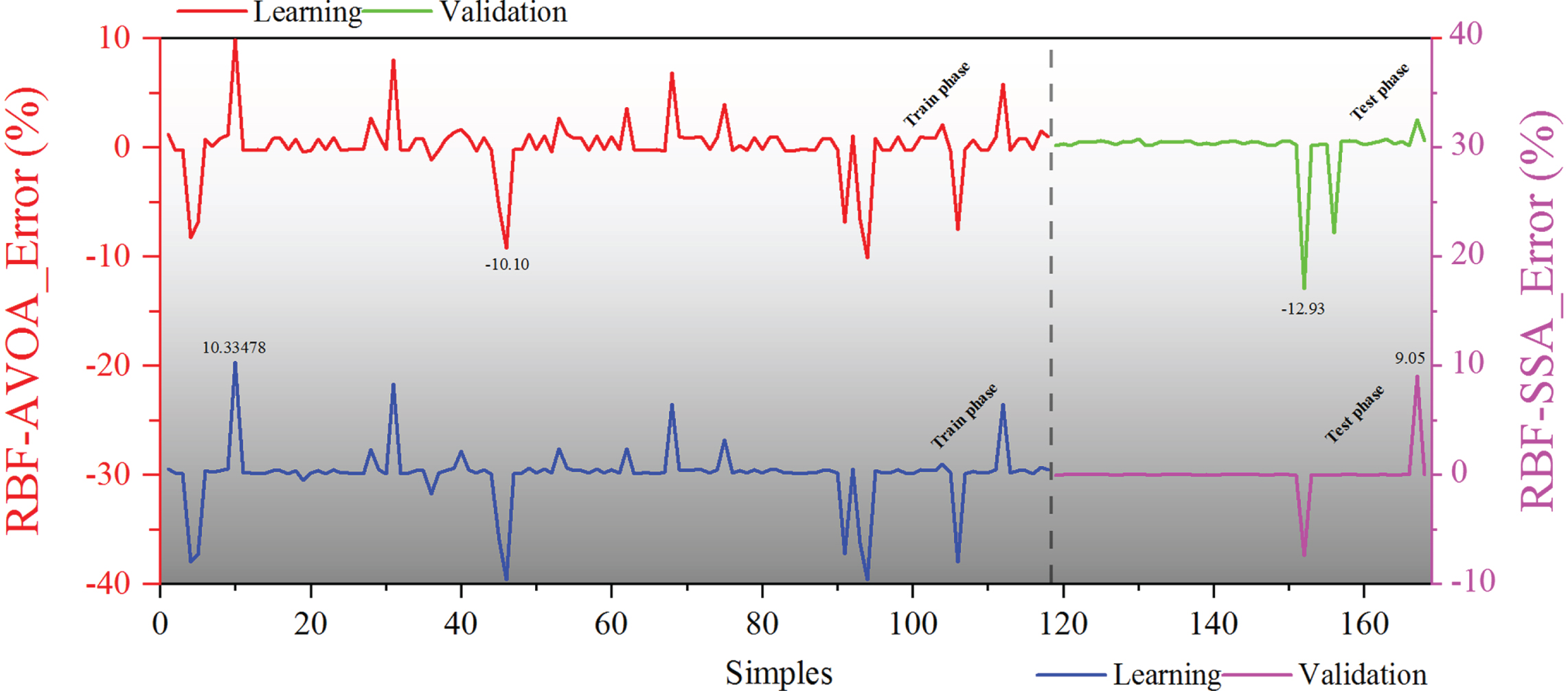
The error percentage diagram of developed models.

In the RBF-SSA model, the fluctuation of the learning part exceeded 10%, and the error values met approximately 10.33%. In the validation phase, the treatment of placing between 10 and –10% is respected by RBF-SSA. However, in the validation section, the RBF-SSA model’s variability is a way that there is no overhang, and it is within range.

A total understanding of Fig. 7 implies that the RBF-SSA model’s behaviour is also better than the RBF-AVOA model, considering the maximum error percentages concentration of error around zero for the RBF-AVOA model is higher than the RBF-SSA model.

Figure 8 shows the two-part error density plots a and b, which characterize the two hybrid models, RBF-AVOA and RBF-SSA. In the RBF-AVOA section, the highest error has a very low-frequency percentage, so the highest error rate is 12%, and the corresponding frequency is almost less than 1%. The peak frequency of this pattern is in the 1-2% range, which indicates the good performance of this model in this area. In section b, related to the combined RBF-SSA model, the highest error rate rises to –14%, where 1% of the samples are in this range, and most are between –1 and 2%. Generally, both models have a percentage error close to zero and give satisfactory results.

Fig. 8

The error percentage density histogram.

Figure 9 illustrates the violin diagram for the error percentage of the developed models. The results indicated that RBF-SSA exhibited the highest dispersion in the learning section, leading to a flattened normal distribution. Conversely, RBF-AVOA demonstrated the highest density in the zero percent range. RBF-AVOA exhibited the highest density in the zero percent range in the validation section, indicating superior accuracy in this domain. It is worth highlighting that RBF-AVOA enhanced its performance by reducing the error in the validation section, whereas RBF-SSA recorded an error exceeding 10%.

Fig. 9

The violin diagram for the error percentage of developed models.

4 Conclusion

Concrete is widely utilized as a building material because of its availability, economical, and widely applicable. High-Performance Concrete production requires supplemental cement-based materials such as high-rate water-reducing agents, silica fume, and fly ash as a binder. Under typical conditions, replacing regular Portland cement with a concrete microfilter can decrease the concrete’s porosity, especially in the long term. Fly ash (FA) is a fine-grained material produced by burning coal to powder in the furnaces of power plants. Silica fume (SF) has two functions: concrete filler and pozzolan. Considering these admixtures increase the hardness of detecting the corresponding compressive strength, and this detection may not be possible by traditional relations.

ANN models have been generated to predict the concrete’s CS. Radial basis function (RBF) neural networks have excellent pattern variety and function-matching capabilities. This is a three-layer forward network. Two optimization algorithms, the African Vulture Optimization algorithm (AVOA) and Salp Swarm Algorithm (SSA), provided the optimal values of RBF structure for better results. To develop the hybrid models, a dataset containing fly ash and silica fume as admixtures were gathered from the literature to improve the hybrid predictive models. The obtained results of two novel hybrid models, RBF-AVOA and RBF-SSA, are compared to have a comprehensive analysis of the models’ performance which are summarized as follows:

The maximum value of R² is equal to 0.9974, which belongs to the combined RBF-AVOA model of the validation section, but the RBF-SSA model of the learning section equal to 0.9851 obtains the minimum value.

The RBF-AVOA model was able to show better performance in RMSE. This corresponds to 0.9191 in the validation section, and the weakest performance from a learning point of view is the RBF-SSA model, which is equal to 0.9851.

For the MAE evaluator, the minimum value is equal to 0.1917, which belongs to the RBF-AVOA model in the validation section, and the maximum value is equal to 0.884, which belongs to the RBF-SSA model in the learning section.

The VAF metric, which should be at the highest level in the combined RBF-AVOA model, has a numerical validation portion equal to 99.7395. The minimum value for this metric is 98.44 in the training portion of the RBF-SSA model.

In general, the hybrid RBF-AVOA model has shown satisfactory and acceptable performance and can be introduced as an applicable model in predicting the compressive strength of high-performance concrete.

Funding

Virtual Reconstruction of Ancient Ceramic Fragments and Research on Cultural Characteristics.

References

Aïtcin

P.-C.

, High performance concrete. CRC press, 1998.

Brandt

A.M.

, Fibre reinforced cement-based (FRC) composites after over 40 years of development in building and civil engineering, Compos. Struct. 86(1–3) (2008), pp. 3–9.

Farnam

, Mohammadi

and Shekarchi

, Experimental and numerical investigations of low velocity impact behavior of high-performance fiber-reinforced cement based composite, Int. J. Impact Eng. 37(2) (2010), pp. 220–229.

Neville

and Aitcin

P.-C.

, High performance concrete— An overview, Mater. Struct. 31(2) (1998), pp. 111–117.

Breitenbuecher

, High performance fiber concrete SIFCON for repairing environmental structures, in Proceedings of the third RILEM/ACI workshop: high-performance fiber reinforced cement composites, London, UK, (1999), pp. 585–594.

Asgeirsson

, Silica fume in cement and silane for counteracting of alkali-silica reactions in iceland, Cem. Concr. Res. 16(3) (1986), pp. 423–428, doi: 10.1016/0008-8846(86)90118-3.

Wesche

, Fly ash in concrete: properties and performance. CRC Press, 1991.

Kuder

K.G.

and Shah

S.P.

, Processing of high-performance fiber-reinforced cement-based composites, Constr. Build. Mater. 24(2) (2010), pp. 181–186, doi: 10.1016/j.conbuildmat.2007.06.018.

Oikonomou

N.D.

, Recycled concrete aggregates, Cem. Concr. Compos. 27(2) (2005), pp. 315–318, doi: 10.1016/j.cemconcomp.2004.02.020.

10.

Schoppe

B.M.

, Shrinkage & modulus of elasticity in concrete with recycled aggregates, 2011.

11.

H.-G.

and Wang

J.-Z.

, Prediction of compressive strength of concrete by neural networks, Cem. Concr. Res. 30(8) (2000), pp. 1245–1250, doi: 10.1016/S0008-8846(00)00345-8.

12.

Lee

S.-C.

, Prediction of concrete strength using artificial neural networks, Eng. Struct. 25(7) (2003), pp. 849–857. doi: 10.1016/S0141-0296(03)00004-X.

13.

Çağlar

, Predicting the compressive strength and slump of high strength concrete using neural network, 2006.

14.

Topcu

I.B.

and Sarıdemir

, Prediction of compressive strength of concrete containing fly ash using artificial neural networks and fuzzy logic, Comput. Mater. Sci. 41(3) (2008), pp. 305–311.

15.

Alshihri

M.M.

, Azmy

A.M.

and El-Bisy

M.S.

, Neural networks for predicting compressive strength of structural light weight concrete, Constr. Build. Mater. 23(6) (2009), pp. 2214–2219.

16.

Bilim

, Atiş

C.D.

, Tanyildizi

and Karahan

, Predicting the compressive strength of ground granulated blast furnace slag concrete using artificial neural network, Adv. Eng. Softw. 40(5) (2009), pp. 334–340.

17.

Chou

J.-S.

, Chiu

C.-K.

, Farfoura

and Al-Taharwa

, Optimizing the Prediction Accuracy of Concrete Compressive Strength Based on a Comparison of Data-Mining Techniques, J. Comput. Civ. Eng. 25(3) (2011),pp. 242–253. doi: 10.1061/(ASCE)CP.1943-5487.0000088.

18.

Atici

, Prediction of the strength of mineral admixture concrete using multivariable regression analysis and an artificial neural network, Expert Syst. Appl. 38(8) (2011), pp. 9609–9618, doi: 10.1016/j.eswa.2011.01.156.

19.

Sobhani

, Najimi

, Pourkhorshidi

A.R.

and Parhizkar

, Prediction of the compressive strength of no-slump concrete: A comparative study of regression, neural network and ANFIS models, Constr. Build. Mater. 24(5) (2010),pp. 709–718. doi: 10.1016/j.conbuildmat.2009.10.037.

20.

Bilim

, Atiş

C.D.

, Tanyildizi

and Karahan

, Predicting the compressive strength of ground granulated blast furnace slag concrete using artificial neural network, Adv. Eng. Softw. 40(5) (2009), pp. 334–340. doi: 10.1016/j.advengsoft.2008.05.005.

21.

Masoumi

, Najjar-Ghabel

, Safarzadeh

and Sadaghat

, Automatic calibration of the groundwater simulation model with high parameter dimensionality using sequential uncertainty fitting approach, Water Supply 20(8) (2020), pp. 3487–3501, doi: 10.2166/ws.2020.241.

22.

Bian

, Zhao

and Wang

, Study on the separation and comprehensive utilization of the hollow microbeads in fly ash, J. China Univ. Min. Technol. 22(2) (1993), pp. 23–30.

23.

Siddique

, Performance characteristics of high-volume Class F fly ash concrete, Cem. Concr. Res. 34(3) (2004), pp. 487– 493. doi: 10.1016/j.cemconres.2003.09.002.

24.

Mehta

P.K.

, High-performance, high-volume fly ash concrete for sustainable development, in Proceedings of the international workshop on sustainable development and concrete technology, 2004, pp. 3–14.

25.

Mazloom

, Ramezanianpour

A.A.

and Brooks

J.J.

, Effect of silica fume on mechanical properties of high-strength concrete, Cem. Concr. Compos. 26(4) (2004), pp. 347–357. doi: 10.1016/S0958-9465(03)00017-9.

26.

Ganesh Babu

and Siva Nageswara Rao

, Early strength behaviour of fly ash concretes, Cem. Concr. Res. 24(2) (1994), pp. 277–284. doi: 10.1016/0008-8846(94)90053-1.

27.

Sabir

B.B.

, Mechanical properties and frost resistance of silica fume concrete, Cem. Concr. Compos. 19(4) (1997), pp. 285–294. doi: 10.1016/S0958-9465(97)00020-6.

28.

Bhanja

and Sengupta

, Influence of silica fume on the tensile strength of concrete, Cem. Concr. Res. 35(4) (2005), pp. 743–747. doi: 10.1016/j.cemconres.2004.05.024.

29.

Mansour

M.Y.

, Dicleli

, Lee

J.-Y.

and Zhang

, Predicting the shear strength of reinforced concrete beams using artificial neural networks, Eng. Struct. 26(6) (2004), pp. 781–799.

30.

K.C.

, Bi

L.P.

and Chen

M.C.

, Prediction model of compressive strength of lithium slag concrete based on SPSS regression analysis, J Arch. Civ Eng 34(1) (2017), pp. 15.

31.

Wen

, Xie

and Pei

, A structure-adaptive hybrid RBF-BP classifier with an optimized learning strategy, PLoS One 11(10) (2016), p. e0164719.

32.

Pala

, Özbay

, Öztaş

and Yuce

M.I.

, Appraisal of long-term effects of fly ash and silica fume on compressive strength of concrete by neural networks, Constr. Build. Mater. 21(2) (2007), pp. 384–394. doi: 10.1016/j.conbuildmat.2005.08.009.

33.

Lam

, Wong

and Poon

, Effect of Fly Ash and Silica Fume on Compressive and Fracture Behaviors of Concrete, Cem. Concr. Res. 28(2) (1998), pp. 271–283. doi: 10.1016/S0008-8846(97)00269-X.

34.

Mirjalili

, Gandomi

A.H.

, Mirjalili

S.Z.

, Saremi

, Faris

and Mirjalili

S.M.

, Salp Swarm Algorithm: A bio-inspired optimizer for engineering design problems, Adv. Eng. Softw. 114 (2017), pp. 163–191. doi: 10.1016/j.advengsoft.2017.07.002.

35.

Madin

L.P.

, Aspects of jet propulsion in salps,”, Can. J. Zool. 68(4) (1990), pp. 765–777.

36.

Henschke

, Everett

J.D.

, Richardson

A.J.

and Suthers

I.M.

, Rethinking the Role of Salps in the Ocean, Trends Ecol. Evol. 31(9) (2016), 720–733, doi: 10.1016/j.tree.2016.06.007.

37.

P.A.V.

and Bone

, Communication between individuals in salp chains. II. Physiology, Proc. R. Soc. London. Ser. B. Biol. Sci. 210(1181) (1980), pp. 559–574. doi: 10.1098/rspb.1980.0153.

38.

Sutherland

K.R.

and Weihs

, Hydrodynamic advantages of swimming by salp chains, J. R. Soc. Interface 14(133) (2017), pp. 20170298, doi:10.1098/rsif.2017.0298.

39.

Mirjalili

, Gandomi

A.H.

, Mirjalili

S.Z.

, Saremi

, Faris

and Mirjalili

S.M.

, Salp Swarm Algorithm: A bio-inspired optimizer for engineering design problems, Adv. Eng. Softw. 114 (2017), pp. 163–191.

40.

Ahmed

, Khamies

, Magdy

and Kamel

, Designing Optimal PIλ D μ Controller for LFC of Two-Area Power Systems Using African Vulture’s Optimization Algorithm, in 2021 22nd International Middle East Power Systems Conference (MEPCON) (2021), pp. 430–437.

41.

Chen

, Fei

and Yuan

, High-performance Concrete Strength Prediction Model Based on the Radial Basis Function Neural Network of Human Cerebral Cortex, NeuroQuantology 16(5), 2018.

42.

, Evaluation of compressive strength of the HPC produced with admixtures by a novel hybrid SVR model, Multiscale Multidiscip. Model. Exp. Des. Mar. 2023. doi: 10.1007/s41939-023-00150-3.

43.

Mousavi

S.M.

, Aminian

, Gandomi

A.H.

, Alavi

A.H.

and Bolandi

, A new predictive model for compressive strength of HPC using gene expression programming, Adv. Eng. Softw. 45(1) (2012), pp. 105–114. doi: 10.1016/j.advengsoft.2011.09.014.

44.

Gandomi

A.H.

and Alavi

A.H.

, A new multi-gene genetic programming approach to nonlinear system modeling. Part I: materials and structural engineering problems, Neural Comput. Appl. 21(1) (2012), pp. 171–187, doi: 10.1007/s00521-011-0734-z.

45.

Asteris

P.G.

, Skentou

A.D.

, Bardhan

, Samui

and Pilakoutas

, Predicting concrete compressive strength using hybrid ensembling of surrogate machine learning models,” Cem. Concr. Res. 145 (2021), pp. 106449, doi: 10.1016/j.cemconres.2021.106449.

46.

Nguyen

N.-H.

, Vo

T.P.

, Lee

and G.

, Asteris, Heuristic algorithm-based semi-empirical formulas for estimating the compressive strength of the normal and high performance concrete, Constr. Build. Mater. 304 (2021), pp. 124467, doi: 10.1016/j.conbuildmat.2021.124467.

47.

Van Dao

, et al., A Sensitivity and Robustness Analysis of GPR and ANN for High-Performance Concrete Compressive Strength Prediction Using a Monte Carlo Simulation,” Sustainability 12(3) (2020), p. 830, doi: 10.3390/su12030830.

48.

Lee

, Nguyen

, Karamanli

, Lee

and Vo

T.P.

, “Super learner machine-learning algorithms for compressive strength prediction of high performance concrete,” Struct. Concr. 24(2) (2023), pp. 2208–2228, doi: 10.1002/suco.202200424.

49.

Zhu

, Huang

and Zhang

, Novel hybrid AOA and ALO optimized supervised machine learning approaches to predict the compressive strength of admixed concrete containing fly ash and micro-silica, Multiscale Multidiscip. Model. Exp. Des. 5(4) (2022), pp. 391–402, doi: 10.1007/s41939-022-00124-x.