Software defect prediction method based on the heterogeneous integration algorithm

Abstract

A software defect is a common cyberspace security problem, leading to information theft, system crashes, and other network hazards. Software security is a fundamental challenge for cyberspace security defense. However, when researching software defects, the defective code in the software is small compared with the overall code, leading to data imbalance problems in predicting software vulnerabilities. This study proposes a heterogeneous integration algorithm based on imbalance rate threshold drift for the data imbalance problem and for predicting software defects. First, the Decision Tree-based integration algorithm was designed following sample perturbation. Moreover, the Support Vector Machine (SVM)-based integration algorithm was designed based on attribute perturbation. Following the heterogeneous integration algorithm, the primary classifier was trained by sample diversity and model structure diversity. Second, we combined the integration algorithms of two base classifiers to form a heterogeneous integration model. The imbalance rate was designed to achieve threshold transfer and obtain software defect prediction results. Finally, the NASA-MDP and Juliet datasets were used to verify the heterogeneous integration algorithm’s validity, correctness, and generalization based on the Decision Tree and SVM.

Keywords

Software defect imbalance rate heterogeneous integration threshold shift

1 Introduction

In recent years, many people have relied on convenient, practical, and robust applications of software functions. Software security is intertwined with daily living and is related to cyberspace security. The factors that cause software insecurity come from the security loopholes caused by the software’s errors, defects, and external attacks. The software’s robustness can be improved, and cyberspace security can resist external attacks if the software is designed to reduce security vulnerabilities and detect defects.

In this case, improving software developers’ capabilities enhances the quality of software products. Investigation into software defects shows an imbalance and fewer defective modules in the software code than defect-free modules. This situation can interfere with the validity of prediction for software defects and make the accuracy of prediction results very challenging. The integrated approach to software defects is currently the most common method to solve the class imbalance problem. This approach effectively improves the final classification results by integrating the strengths of individual learners [1, 2]. All base classifiers are of the same importance, and the higher the difference between the results, the better the integrated model effect.

The integration comprises homogeneous integration and heterogeneous integration, according to the same individual classifiers. Homogeneous integration shows that the integrated individual classifier groups are all the same. In machine learning [3], homogeneous integration algorithms comprise the current popular algorithm of Random Forest, ExtraTrees, and Gradient-Boosted Decision Trees (GBDT). The Classification and Regression Trees (CART) are the base classifiers of these three integrated algorithms. Enhancing the diversity of basic classifiers is the key to improving the generalization ability of ensemble learning. The enhancement methods include data, parameters, and model structure. However, homogeneous integration does not consider the model structure diversity [4]. Heterogeneous integration is a method that combines different types of machine learning algorithms to improve the accuracy and robustness of the model. However, performance bottlenecks may occur because of the vast structural differences between heterogeneous classifiers, resulting in the difficulty of integration and the performance degradation of the entire algorithm. Therefore, this study explores the heterogeneous integration algorithm.

Three main problems with software defects are as follows: (1) the imbalance of defect data in software needs must be considered; (2) the classifier structural diversity is not considered in the research using an isomorphic integration algorithm; and (3) heterogeneous integration algorithms cannot guarantee integration algorithms’ performance and generalization ability. This study proposes a Software Defect prediction method based on Heterogeneous Integration algorithms (SDHetInt) to improve the effectiveness and generalization ability of the integration algorithm on imbalanced datasets. In response to the three above-mentioned problems, this article proposes a SDHetInt integration algorithm. Compared with the currently popular isomorphic ensemble algorithms such as Random Forest, ExtraTrees, and GBDT, SDHetInt uses different machine learning models to construct the basic classifier, considers the diversity of data samples and input attributes, and moves the threshold based on the imbalance rate of defect data. Compared with single machine learning models and isomorphic ensemble algorithms, the SDHetInt heterogeneous ensemble algorithm can effectively solve the problem of low defect prediction performance caused by data imbalance by predicting software defects.

This study provides the following contributions:

We analyze the correlation between software features and defects based on unbalanced software defect data. Sample perturbation and attribute perturbation construct two software defect classifiers with different structures.

A SDHetInt heterogeneous integration classifier is constructed using software defect classifiers with different structures. The results of predicting software defects in NASA datasets show that the SDHetInt heterogeneous integration classifier offers a good prediction effect on unbalanced data processing. Moreover, SDHetInt offers better heterogeneous integration algorithm performance than the current popular Forest, ExtraTrees, GBDT integration algorithm, and isomorphic integration algorithm.

We achieved good prediction results by applying the SDHetInt heterogeneous integration classifier to NASA and Juliet’s unbalanced software defect data. The proposed SDHetInt has excellent generalization ability.

The rest of this paper is organized as follows. Section 2 describes the related work. Section 3 discusses the heterogeneous integration method and algorithm, including constructing the Decision Tree and Support Vector Machine (SVM) based classifier, the fusion of the base classifier, and the threshold shift based on the imbalance rate. Section 4 describes our experimental evaluation and the results of SDHetInt. Section 5 discusses the limitations of SDHetInt and problems to be addressed in future research. Section 6 presents the conclusions.

2 Related work

Data security has garnered increasing attention due to the frequent occurrence of network security events. Software defect prediction is a meaningful way to analyze software quality and reduce development costs. Software defect prediction is a research problem in the field of software engineering. Many research achievements have been made, which have occupied a leading position in software security [5–9]. Software defect analysis includes static, dynamic, and dynamic static combination analysis methods. The static analysis method consists of the static analysis of source and binary codes. Dynamic analysis and dynamic static combination analysis are used to analyze binary files.

Due to the binary software limitation, most current research applies the static analysis of software source code to predict software defects. At the initial stage of software development, Czibula et al. [10] proposed a model of relationship association discovery based on software defect prediction. They applied and compared all the NASA datasets with other evaluation models. They have better accuracy, specificity, and detection probability and cover evaluation prediction results. In a previous study on software defect prediction, supervised learning consumes considerable effort when labeling training data.

Patil et al. [11] used explicit semantic analysis to classify software defect reports based on concepts, analyze the source code’s semantic information, and predict software defects. This method determines the semantic similarity between the defect type label defect report in the conceptual space of Wikipedia. Then, this method assigns the defect type with the highest similarity to the defect report. However, in the practical field of software development, the software projects that must be predicted are usually brand-new software projects that need more labeled data to build defect prediction models. Zhao et al. [12] proposed a cross-project defect prediction method based on stream feature transformation in cross-project software. Currently, several studies have proposed on-the-fly techniques to predict defective changes. Ardimento et al. [13] proposed an on-the-fly software defect prediction technique based on temporal convolutional networks using features from source code metrics detected in the commit history of software projects. Ardimento et al. [14] proposed a comprehensive feature set approach that can promptly predict the defect propensity of code components and improve the performance of the on-the-fly defect prediction model. Table 1 summarizes the related work on software defect prediction.

Table 1
The related work on software defect prediction

Research articles Year Type Testbeds Algorithm Assessment

S. Wahono [5] 2015 Review

B. Zhang [6] 2020 Review

J. Pachouly [7] 2022 Review

B. Khan [8] 2021 Article AR1, AR3, CM1, JM1, KC2, KC3, MC1 MLP, SVM, J48, RBF, RF, HMM, CDT, KNN, A1DE, NB RAE, MAE, RMSE, RRSE, Recall, Accuracy

D. L. Miholca [9] 2020 Article JEdit 3.2, JEdit 4.0, JEdit 4.1, JEdit 4.2, JEdit 4.3, Ant 1.7, Tomcat 6.0 Doc2Vec, LSI, LR, KNN, ANN LOO, ROC

G. Gzibula [10] 2014 Article MW1, JM1, PC1, PC2, PC3, PC4, KC1, KC3, MC2, and CM1 READ Accuracy, Specificity, Precision, PD, and ROC

S. Patil [11] 2020 Article Apache-Libs, Roundcube LeDEx, SVM, CBC Precision, Recall, and F1 score

Y. Zhao [12] 2021 Article Relink, AEEEM Naive Bayes F1 score

P. Ardimento [13] 2020 Article Log4j, Javassist, JUnit4, ZooKeeper TCN Accuracy, F-measure

P. Ardimento [14] 2022 Article six open-source projects TCN, LSTM, TPE, SBMO Precision, Recall, and F1 score

Research articles	Year	Type	Testbeds	Algorithm	Assessment
S. Wahono [5]	2015	Review
B. Zhang [6]	2020	Review
J. Pachouly [7]	2022	Review
B. Khan [8]	2021	Article	AR1, AR3, CM1, JM1, KC2, KC3, MC1	MLP, SVM, J48, RBF, RF, HMM, CDT, KNN, A1DE, NB	RAE, MAE, RMSE, RRSE, Recall, Accuracy
D. L. Miholca [9]	2020	Article	JEdit 3.2, JEdit 4.0, JEdit 4.1, JEdit 4.2, JEdit 4.3, Ant 1.7, Tomcat 6.0	Doc2Vec, LSI, LR, KNN, ANN	LOO, ROC
G. Gzibula [10]	2014	Article	MW1, JM1, PC1, PC2, PC3, PC4, KC1, KC3, MC2, and CM1	READ	Accuracy, Specificity, Precision, PD, and ROC
S. Patil [11]	2020	Article	Apache-Libs, Roundcube	LeDEx, SVM, CBC	Precision, Recall, and F1 score
Y. Zhao [12]	2021	Article	Relink, AEEEM	Naive Bayes	F1 score
P. Ardimento [13]	2020	Article	Log4j, Javassist, JUnit4, ZooKeeper	TCN	Accuracy, F-measure
P. Ardimento [14]	2022	Article	six open-source projects	TCN, LSTM, TPE, SBMO	Precision, Recall, and F1 score

2.1 Category unbalanced prediction method

In the current software development environment, the size of software code data increases as the software becomes more complex. Since the software code with fewer defects is higher than the code without defects, an imbalance is noted when predicting defects. This issue makes data classification difficult. Most algorithms focus on classifying primary samples while ignoring or mistakenly classifying a few samples. The class imbalance has become the biggest problem in data mining. Machine learning uses five technologies for processing unbalanced data: oversampling, undersampling, cost-sensitive learning, ensemble learning, and combined class methods [15–19]. Oversampling is balanced by increasing the size of rare samples. SMOTE is the primary technique of oversampling. This method is limited based on the assumption that the local space between two positive instances belongs to a few classes and that the training data are not linearly separable. This assumption may sometimes be correct. Undersampling processes of an unbalanced dataset are critical by reducing the number of classes. Cost-sensitive learning adds misclassification costs by minimizing the total cost. This technology aims to achieve high accuracy when classifying instances into a group of known classes. Integrated learning technology combines multiple classifiers to improve the performance of a single classifier. This method modifies the inductive ability of a single classifier by assembling different classifiers. It also incorporates the output of multiple primary learners. The composite class method is to combine various techniques.

In predicting software defects, some studies use oversampling or undersampling to balance datasets and solve the problem of category imbalance. Goyal proposed a neighborhood-based undersampling algorithm to solve the class imbalance problem [20]. The algorithm under-samples the dataset to maximize the visibility of a few data points while limiting the excessive elimination of most data points to avoid information loss. Other scholars solve the problem of category imbalance in predicting software defects. Aankush et al. used a combination of simple noise removal, unbalanced class distribution, and software metric selection techniques to optimize defect prediction in software [21]. Pandey et al. manually added various noise levels and determined their impact on the performance of software defect prediction models [22]. They devised techniques to guide the baseline model’s possible range of allowable noise. Liu et al. proposed a weighted Gini coefficient embedding feature selection method to solve the category overlapping problem [23].

Some scholars predict software defects based on distance metrics to solve the category imbalance problems. Jin proposed a distance-measure learning method based on cost-sensitive learning to reduce the impact of sample category imbalance. They applied this technique to the sizeable marginal distribution machine to replace the traditional kernel function [24]. The CS-ILDM model is proposed to predict the defects in software. The improvement and optimization of Large margin Distribution Machine based on Cost-Sensitive Learning are used to predict software defects. Chakraborty et al. proposed a hybrid method of the Hellinger network model [25]. Hellinger network is a tree-to-network mapping model and a deep feed-forward neural network with a built-in hierarchical structure. This method improves software defect prediction based on an insensitive skew distance metric when dealing with class imbalance problems.

To be more robust than using absolute distance information to predict software defects, Zheng et al. introduced the relative density to reflect the importance of each instance in their class. They used the probability density estimation based on the K-nearest neighbor to calculate the relative density of each training instance. They also designed the fuzzy membership degree of the sample based on the relative density to predict the defects of the software [26]. Table 2 summarizes the methods to solve the category imbalance.

Table 2
The methods to solve the category imbalance

Research articles Year Testbeds Algorithm Assessment

S. Goyal [20] 2021 CM1, JM1, KC1, KC2 and PC1 N-US Confusion matrix, ROC, AUC, Accuracy, and recall

J. Aankush [21] 2020 Framework, jdt, lucene, Mylyn, pde, jm1, kc1, kc2, pc1, pc3 NB, LR, SVM, RF, XGBoost Accuracy, Precision, Recall, F-measure, AUC

S. K. Pandey [22] 2021 Columba, Scarab, Eclipse NB, LSVM, J48, AdaBoost, RF TPR, FPR, ROC

H.Y. Liu [23] 2019 Statlog, Letter recognition xgboost AUC, ROC

C. Jin [24] 2020 NASA LDM, NB, C4.5, RCSSVM, ANN-ABC, SMOTE, CS-KLDM,CS-ILDM Pd, pf, bal, G-mean, AUC

T. Chakraborty [25] 2020 NASA Hellinger Recall, AUC, and F-measure

S. Zheng [26] 2020 PROMISE KNN-PDE, NB, RF G-mean, AUC, Balance

Research articles	Year	Testbeds	Algorithm	Assessment
S. Goyal [20]	2021	CM1, JM1, KC1, KC2 and PC1	N-US	Confusion matrix, ROC, AUC, Accuracy, and recall
J. Aankush [21]	2020	Framework, jdt, lucene, Mylyn, pde, jm1, kc1, kc2, pc1, pc3	NB, LR, SVM, RF, XGBoost	Accuracy, Precision, Recall, F-measure, AUC
S. K. Pandey [22]	2021	Columba, Scarab, Eclipse	NB, LSVM, J48, AdaBoost, RF	TPR, FPR, ROC
H.Y. Liu [23]	2019	Statlog, Letter recognition	xgboost	AUC, ROC
C. Jin [24]	2020	NASA	LDM, NB, C4.5, RCSSVM, ANN-ABC, SMOTE, CS-KLDM,CS-ILDM	Pd, pf, bal, G-mean, AUC
T. Chakraborty [25]	2020	NASA	Hellinger	Recall, AUC, and F-measure
S. Zheng [26]	2020	PROMISE	KNN-PDE, NB, RF	G-mean, AUC, Balance

2.2 Machine learning integration method

Due to their advantages in solving unbalanced data, integration algorithms have been used to predict software defects. The integration methods based on machine learning comprise isomorphic integration and heterogeneous integration. Most studies focus on isomorphic integration algorithms based on feature selection and bagging strategy.

In integration methods based on machine learning, some scholars have proposed methods based on feature selection. Jiang et al. proposed a feature selection method based on sorting integration to avoid the instability of standard sorting feature selection [27]. They used a logical regression algorithm to build prediction models for frequent redundant or irrelevant features in defect datasets.

Bagging integration algorithms are used based on machine learning. Iqbal et al. proposed an integrated classification framework based on MLP for predicting software defects by using three dimensions: tuned MLP, tuned MLP with bagging technology, and tuned MLP with pressurization [28]. Mousavi et al. predicted software defects by integrating bagging and static and dynamic integration selection strategies [29]. This method uses a new packaging method for category imbalance learning.

In researching heterogeneous integration algorithms, some scholars have adopted the method of constructing new datasets. For example, Yu et al. analyzed the impact of class balance on model performance [30]. They showed that the performance of many personal classifiers will decrease with an increase of unbalance rate. However, the performance of logistic regression and stochastic forest model is superior to that of other algorithms, proving the integration algo-rithm’s accuracy based on the decision tree. Table 3 summarizes the integration methods in machine learning.

Table 3
The integration methods in machine learning

Research articles Year Testbeds Algorithm Assessment

L. Jiang [27] 2018 NASA LR AUC

A. Iqbal [28] 2020 NASA MDP Bagging-MLP Accuracy, F-measure, AUC, MCC

R. Mousavi [29] 2018 NASA Over-Bagging G-mean, balance, AUC

Q. Yu [30] 2018 PROMISE LR, NB, RF AUC

Research articles	Year	Testbeds	Algorithm	Assessment
L. Jiang [27]	2018	NASA	LR	AUC
A. Iqbal [28]	2020	NASA MDP	Bagging-MLP	Accuracy, F-measure, AUC, MCC
R. Mousavi [29]	2018	NASA	Over-Bagging	G-mean, balance, AUC
Q. Yu [30]	2018	PROMISE	LR, NB, RF	AUC

3 SDHetInt Heterogeneous integration method

Although deep learning models can achieve excellent results in classification algorithms, they require massive datasets and high-performance intensive computing hardware. Small sample data are required to demonstrate software defects because of data imbalance when predicting software defects. Thus, traditional machine learning has better performance and offers hardware resource efficiency advantages.

Different from isomorphic integration algorithms such as Random Forest, ExtraTrees, and GBDT, as well as using the method of constructing new datasets to construct heterogeneous integration algorithms. Based on the current research on integration algorithms, this study proposes a heterogeneous integration method based on imbalanced rate threshold shifts to predict software defects and handle imbalanced software defect data. Machine learning algorithms are an appropriate choice when selecting a primary classifier for predicting software defects because they are fast, efficient, robust to noisy data, and suitable for binary classification and high-dimensional data.

In addition to meeting the above advantages, the calculation amount of the Decision Tree is relatively small, and it is easy to convert into classification rules. Decision Tree can also handle continuous and category fields insensitive to missing values and irrelevant features. It only needs one construction and can be used repeatedly. The maximum number of calculations for each prediction is the depth of the Decision Tree. SVM can use kernel function to map to high-dimensional space. When dealing with prediction defects, SVM can solve the nonlinear classification of binary classification and avoid features such as over-fitting and generalization errors in Decision Trees. Therefore, this study selects Decision Tree and SVM model with significant differences to build two sets of basic classifiers. Then, a heterogeneously integrated classifier is constructed based on the fusion of two basic classifiers.

The algorithm comprises three parts: (1) data on software defects were preprocessed to select features more effectively to predict software defects. (2) Based on software defect data training, a group of decision tree classifiers with diversity was trained using sample disturbance. A group of SVM classifiers with diversity was trained using attribute disturbance. (3) Two sets of base classifiers were combined, and the prediction of two sets of base classifiers was considered as the probability value of defect samples. The final prediction probability value of the heterogeneous ensemble algorithm was obtained through a simple average method. Based on the imbalance rate, a threshold was set, and the samples with a probability more significant than the threshold were classified as defect samples. In comparison, the samples with a probability less than the threshold were classified as non-defect samples. Figure 1 shows the specific process.

Fig. 1

Software defect prediction framework based on heterogeneous integration.

3.1 Data preprocessing

Software measurement is a quantitative measurement technique for software projects, development processes, and software products [31, 32], which provides a quantitative standard for evaluating code quality. The structured software metrics method is an example of the quantitative software method. Among the classical structured metric methods of program software, the metrics methods based on line of Code, Halstead, McCabe, Cyclomatic Complexity, Essential Complexity, Design Complexity, Integration Complexity, C&K, and MOOD have been proven to predict software defects accurately and efficiently [33–35]. This study establishes a defect prediction model based on the structured software metrics method. The study predicts defects in software based on Halstead, Cyclic Complexity, Essential Complexity, Design Complexity, and other metrics methods. See Section 4.1 for details.

Analyzing the internal correlation between each feature and defect category is vital because software defects contain many duplicate data. This approach effectively reduces the feature dimension and improves the algorithm’s operation efficiency.

The historical data preprocessing of software defects is as follows: (1) the first step is to delete the duplicate data samples in the historical data. Deleting will include features with zero values, missing values, and the same feature values. (2) Second, the relationship between features and software defect categories is analyzed. According to the filtering method, feature selection is performed on the dataset. Selecting the feature corresponding to the software defect category as the feature subset is essential.

Common external features of the software include lines of code, lines of declaration class code, lines of execution class code, number of function nesting levels, program execution path, and cyclomatic calculation complexity. Common internal features of the software include function names and function calls in the source code. The univariate feature selection of the filter selection method consists of the Chi-square test, Pearson’s correlation coefficient, and mutual information. Pearson’s correlation coefficient feature selection is a method that can analyze the relationship between features and response variables. This method measures the linear correlation between variables. Thus, we chose the Pearson’s correlation coefficient for feature selection. When Pearson’s correlation coefficient is used to measure the relationship between features and categories in the data on software defects, the larger the value, the stronger the correlation between features and categories. The feature is strongly correlated, as shown in Equation (1):

$ρ (X, Y) = \frac{\sum_{i = 1}^{n} (X - μ_{x}) (Y - μ_{y})}{\sqrt{\sum_{i = 1}^{n} {(X_{i} - μ_{x})}^{2}} \sqrt{\sum_{i = 1}^{n} {(Y_{i} - μ_{y})}^{2}}}$ (1)

where X represents software features; Y represents whether the software contains defects, and n is the total number of samples. X_i represents the feature of the ith sample. Y_i represents the category label of the ith sample; μ_x is the mean value of X; and μ_y is the mean of Y. $\sum_{i = 1}^{n} (X - μ_{x}) (Y - μ_{y})$ is the covariance of X and Y. $\sqrt{\sum_{i = 1}^{n} (X_{i} - μ_{x})^{2}}$ represents the standard deviation of X, and $\sqrt{\sum_{i = 1}^{n} (Y_{i} - μ_{y})^{2}}$ represents the standard deviation of Y. Covariance represents the direction of correlation between two variables. However, the interpretation strength has a dimension problem. In (1), the covariance is divided by the standard deviation of x and the standard deviation of Y. The range of (X, Y) is [– 1, 1], where 1 represents the complete positive correlation between features and software defects; 0 represents no linear correlation between features and software defects, and – 1 represents the complete negative correlation between features and defects. The closer the correlation coefficient is to 1, the stronger the positive correlation between software features and defects. Therefore, we calculate the correlation between features and software defects and select features with a strong correlation as the feature subset of software defect prediction. See Section 4.3.1 for detailed analysis results.

After deduplication and feature selection, this paper divided the feature subset of software defect history data into DDT and DSVM. The DDT and DSVM datasets were divided into several sub-datasets according to the corresponding number of base classifiers. Thus, randomness was introduced into the homogeneous individual classifier to enhance the diversity of individual learners and build an ensemble classifier with strong generalization ability. Additionally, two data samples and attribute disturbance methods were selected to improve diversity.

Data sample disturbance is usually based on the sampling method. When classifiers such as the decision tree and neural network change slightly in the training samples, the learners will change significantly. Therefore, the data sample disturbance is very effective for this unstable base learner. The dataset DDT={DDT1, DDT2, \dots , DDTn} and these sub-datasets were used to train different decision tree classifiers’ IDT.

Since SVM belongs to a stable classifier and is insensitive to the disturbance of data samples, input attribute disturbance is adopted for SVM. Different attribute sub-datasets were generated in the DSVM dataset DSVM={DSVM1, DSVM2, \dots , DSVMn} according to the input attribute disturbance method. These sub-datasets were used to train different SVM classifiers for ISVM.

3.2 Construction base classifier

3.2.1 Construction of the decision tree base classifier

We obtained a subset of a specific defect training data sample size through resampling. Then, we randomly extracted a fixed number of defect attributes from the obtained training subset to allow the base classifier to be as diverse as possible in the training stage of the base classifier of the decision tree. Multiple defect training subsets for DDT were obtained by sample disturbance in the training set {DDT1, DDT2, \dots , DDTn} and input to the decision tree base classifier for training. Finally, a set of base classifiers with improved generalization performance IDT={IDT1, IDT2, \dots , IDTn} was obtained.

A decision tree algorithm is a tree structure that classifies instances based on features. The decision tree has two types of nodes: internal nodes and leaf nodes. Internal nodes represent attributes in software defect data, such as code lines, the number of operators, and cyclomatic complexity. Leaves indicate whether the software code module has defects. During classification, the decision tree starts from the root node to test the attributes of the test sample, and each internal node corresponds to the value of a feature. According to the test results, the sample is analyzed to the branch node of the lower level, which is a recursive process until the sample reaches the leaf node, and the corresponding category is obtained.

The construction process of a decision tree-based classifier includes decision tree generation and pruning. The detailed process is as follows:

Generation of Decision Trees: For software defect classification, the generation of the decision tree is a top-down, divide-and-conquer process, which is essentially a greedy algorithm. Measuring the training dataset for testing is vital, starting from the root node for each leaf node. According to the different test results, the dataset is divided into training sets. Each child training set constitutes a new non-leaf node. The above process is repeated and divided until the termination conditions are met to form a leaf node. Thus, we use the Gini index to measure the impurity of the data partition D.

Pruning of Decision Trees: The cost complexity pruning algorithm is used to prune the tree. In this process, the tree complexity is a function of the number of leaf nodes in the tree and the error rate of the tree. Starting from the bottom of the tree, for each internal node N corresponding to a software defect feature, the subtree of N and the cost complexity of the subtree of N after pruning are calculated to decide whether to prune.

The decision in the algorithm takes the Gini coefficient as the splitting point of the metric index. The training dataset D is divided into D1 and D2, depending on whether the metric index F takes a certain possible value. Under metric index F, the Gini index definition of set D is shown in Equation (2).

$\begin{matrix} Gini (D, F) \\ = \frac{\sum_{i = 1}^{n} (X - μ_{x}) (Y - μ_{y})}{\sqrt{\sum_{i = 1}^{n} {(X_{i} - μ_{x})}^{2}} \sqrt{\sum_{i = 1}^{n} {(Y_{i} - μ_{y})}^{2}}} \end{matrix}$ (2)

The Gini index Gini(D, F) shows the uncertainty of set D after F = fi segmentation. The sample’s uncertainty is higher with a larger Gini index. Finally, the single decision tree model is trained to predict defects in the software code module through the test set indicators.

The above is the generation process of a single decision tree. Several trees with different structures must be trained to obtain a set of IDT base classifiers, as shown in Fig. 2. Since each tree is trained from random sampling and random attribute extraction, the independence of each tree is guaranteed.

Fig. 2

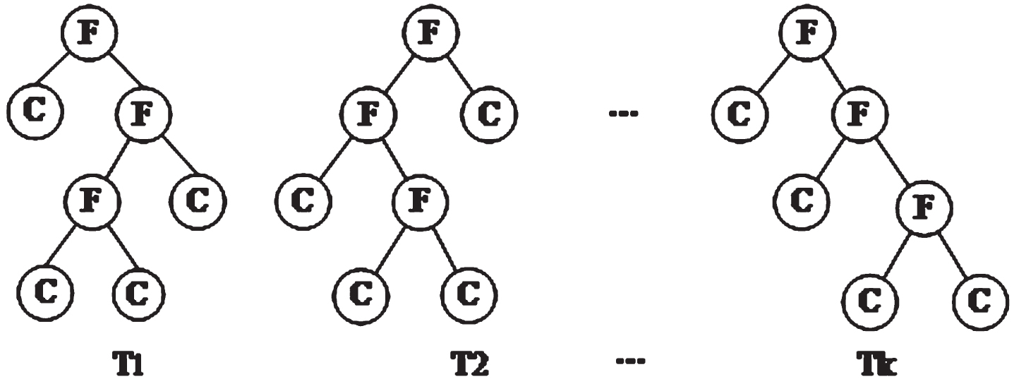
Composition of the decision tree integration model.

Pseudocode 1 introduces the construction process of the IDT basic classifier. Pseudocode 2 introduces the construction process of the decision tree. When the number of decision trees is N, the training sample set of software defects is set as D={(x₁, y₁), (x₂, y₂), \dots , (x_n, y_n)}. After random sampling and random extraction of attributes, the newly generated sub-training set becomes D_i, D_i ⊆ D, Software Metrics Set F={f₁, f₂, \dots , f_n} and F_i is the metric set in the newly generated sub-training set D_i. F_i ⊆ F.

Pseudocode 1. Construction of the IDT base classifier
Input:	D, N
Output:	Multiple decision tree sets {h_i, i = 1,2,3,…, N}, H(x)
1.	fori = 1,2,3,..., N
2.	D_i ← Randomly selected attributes (D)
3.	Pseudocode 2, h_i ← Without pruning (D_i)
4.	end for
5.	h₁(x), h₂(x),..., h_N(x) ← Prediction(N, x)
6.	$H (x) = \frac{1}{N} \sum_{i = 1}^{N} h_{i} (x)$
7.	Return H(x)

Pseudocode 2. Construction of the decision tree
Input:	D_i, F
Output:	A decision tree
1.	create a node q
2.	if D_i ∈ C then
3.	Return q ← C
4.	end if
5.	if F_i=Φ then
6.	Return q ← Most classes (D_i)
7.	end if
8.	best_f ← Select attribute (Gini, F_i)
9.	best best_f ← q
10.	for value q_i in each best_f
11.	a branch ← q (best_f = fi)
12.	S_i={best_f = f_i in F_i}
13.	end for
14.	if Si=Φ then
15.	Add a leaf ← Most class (F_i)
16.	Else
17.	Add a node ← Generate_DT (D_i, F_i)
18.	end if
19.	Return A decision tree

Lines 1–4 of Pseudocode 2 create a decision tree; lines 5–7 create the leaf node that carries the defect category; lines 8–9 look for the best features to divide the defect dataset; and lines 10–18 recursively create a decision subtree for each partitioned defect dataset. Pseudocode 1 calls Pseudocode 2 several times to generate multiple decision trees. Line 5 conducts a simple average based on the prediction results of the created multiple Decision Trees to obtain the probability value predicted as the defective category. A set of decision tree base classifiers, constructed by traversal Pseudocode 2, outputs the probability values of positive classes after voting all Decision Trees.

3.2.2 Construction of support vector machine classifier

Independence should enhance the diversity of the base classifier. In the training stage of the SVM integrated model, multiple defect training subsets DSVM were obtained through attribute disturbance in the training set DSVM={DSVM1, DSVM2,..., DSVMn}. By inputting the sub-dataset into the SVM base classifier for training, a set of base classifiers with improved generalization performance, ISVM={ISVM1, ISVM2,..., ISVMn}, is obtained. In the classifier, software defects are predicted by the decision boundary of the SVM to learn the maximum margin hyperplane of software defect samples. Figure 3 shows the detailed principle of SVM.

Fig. 3

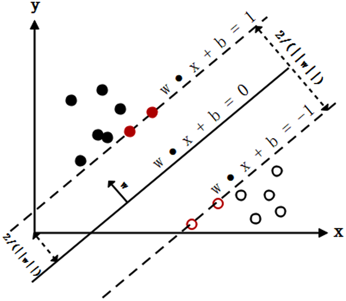
Principle of the support vector machine.

When predicting software defects, the dataset is D={(x₁, y₁), (x₂, y₂),..., (x_N, y_N)}. Each input data sample contains multiple software defect features, and the feature is X_i =[X₁, X₂,..., X_N] ∈ X = Rⁿ, thereby forming the feature space. The classification target is the binary variable y ∈ Y={– 1, 1}, where y indicates no software defect or software defect. $w^{T} X + b = 0$ (3) $y_{i} (w^{T} X_{i} + b) ⩾ 1$ (4)

X_i in Equations (3) and (4) is the defect feature of the ith sample; y_i indicates whether the ith sample contains defects; w is the normal vector of the hyperplane; and b is the intercept of the hyperplane. The decision boundary satisfying this condition constructs two parallel hyperplanes used as interval boundaries to determine whether the software contains defects. Solving the separation hyperplane and classification decision function is as follows: first, the penalty parameter C > 0 is selected to construct and solve the convex quadratic programming problem. $min_{α} \frac{1}{2} \sum_{i = 1}^{N} \sum_{j = 1}^{N} α_{i} α_{j} y_{i} y_{j} (x_{i} \cdot x_{j}) - \sum_{i = 1}^{N} α_{i}$ (5) $s . t . \sum_{i = 1}^{N} α_{i} y_{i} = 0$ (6) $0 ⩽ α_{i} ⩽ C, i = 1, 2, . . ., N$ (7) N in the formula is the total number of predicted software defect data samples. C is the penalty parameter. The optimal solution α_i^* is obtained by Equations (5)–(7), and the separation hyperplane is solved by Equations (8) and (9). $w^{*} = \sum_{i = 1}^{N} {α_{i}}^{*} y_{i} (x_{i} \cdot y_{i})$ (8) $b^{*} = y_{i} - \sum_{i = 1}^{N} {α_{i}}^{*} y_{i} (x_{i} \cdot y_{i})$ (9)

The above is the training process of a single SVM model, in which the feature space X_i =[x₁, x₂,..., x_n] is the set of feature attributes based on software metrics. Each SVM is trained from a new data subset with random sampling and attribute disturbance. A set of highly independent SVM base classifiers is obtained.

When the number of SVM algorithms is M, the training sample set of software defects is set as D={(x₁, y₁), (x₂, y₂),..., (x_n, y_n)}. After random sampling and random attribute extraction, the newly generated sub-training set becomes D_i, D_i ⊆ D; the probability of test sample x is W(x), and a logical regression model is w_j. Pseudocode 3 introduces the construction process of the ISVM basic classifier, and Pseudocode 4 introduces the construction process of the SVM classifier.

Pseudocode 3. Construction of the ISVM base
classifier
Input:	D, N
Output:	Multiple support vector machine {w_j, j = 1,2,3,...,
M }, W(x)
1.	forj = 1,2,3,...,M
2.	D_i ← Randomly selected attributes (D)
3.	Pseudocode 4, w_j ← Train (D_i)
4.	end for
5.	W₁(x), W₂(x),...,W_M(x) ← Predict (M,x)
6.	$W (x) = \frac{1}{M} \sum_{j = 1}^{M} w_{j} (x)$
7.	Return W(x)

Pseudocode 4. Construction of the ISVM base
classifier
Input:	D_i
Output:	support vector machine classifier
1.	Select penalty parameter C > 0, calculate
Equations (5)–(7)
2.	Get α^* = (α₁^, α₂^, . . . , α_N^*) ^T
3.	calculate Equation (8)
4.	Select a component α_j^* ∈ α^, 0 ⩽ α_j^ ⩽ C to calculate
Equation (9)
5.	find separated hyperplanes
6.	if W^TX_i + b > = + 1, ⟶ y_i = + 1 then
7.	classified ← defects
8.	Else
9.	classified ← no defect
10.	end if

3.3 Construction of the defect prediction model

3.3.1 Combining multi-base classifiers

After the above training process, the trained IDT and ISVM base classifiers were obtained, and the two base classifiers were combined to form a heterogeneous integration algorithm. Combining multiple disturbance mechanisms makes the differences between base classifiers more significant. The effect of the classifier is improved with an increase in the degree of difference between individual learners.

The combination methods of classifiers are in two categories: the first is based on the construction of classifiers, and the second is based on the output of classifiers. We use the second method to calculate the classification to obtain a better prediction effect.

The single base classifier generated by the training samples outputs a probability of the category predicted to have defects for each sample in the defect test set. The output result of the final strong classifier is calculated using the probability value of all the internal single-base classifiers. The calculation is as follows: $P = \frac{1}{n} \sum_{i = 1}^{n} P_{i} (y = 1 | x)$ (10) where n represents the number of base classifiers, and P_i (y = 1 | x) represents the probability that the base classifier predicts a defective category. The adopted combination strategy is the simple average strategy, judged according to the average value of probability values of each type predicted by each decision tree or each SVM. Since defect prediction is a binary classification problem, each base classifier’s probability of predicting the defect category can be determined. Then, the average value of this category is obtained.

3.3.2 Threshold shift based on imbalance rate

With great differences, two groups of base classifiers IDT and ISVM were built into heterogeneous integration models by setting the imbalance rate for threshold movement. This section introduces the predicted probability values obtained from each model with the imbalance rate for prediction.

In the dichotomy problem of software defects, the classifier’s probability of predicting defects is P, and the probability value of no defects is 1– P. M is the ratio of two categories of probabilities, called the odds ratio or probability, as shown in Equation (11). $M = \frac{P}{1 - P}$ (11)

The imbalance rate K is defined according to the proportion of categories in software defect data. In the data, the number of samples with defects is m, and the number of samples without defects is n. The imbalance rate is shown in Equation (12). $K = \frac{m}{n}$ (12)

This value is also known as the observed probability of defect data, M’=K. In algorithm classification, the samples will be classified into defective categories when the prediction probability M is greater than the actual observation probability M’. Meanwhile, (13), (14) are further calculated. $\frac{p}{1 - p} ⩾ \frac{m}{n}$ (13) $P ⩾ \frac{m}{n + m}$ (14)

When the classifier makes a prediction, two types of samples will reach equilibrium based on default. Thus, the observation probability is 0.5; the threshold value of the classifier defaults to 0.5. When it is more significant than 0.5, it is a defect class; when it is less than 0.5, it is a non-defect class. However, the defect data could be more balanced. It will also disturb the effectiveness of the prediction algorithm and bring significant challenges to the accuracy of the prediction results. Therefore, adjusting the decision rules is critical through the threshold movement. Adopting the original unbalanced historical defect samples is also essential for learning. In the prediction of the trained classifier, the observation probability of the historical defect samples was used as a new threshold to alleviate the influence of unbalanced data on the classifier.

First, the output results of the base classifier are counted. Then, the integration strategy of soft voting for probability is adopted. The IDT and ISVM base classifiers are combined into a final robust classifier using a simple average fusion strategy. According to the data of software defects, the unbalance rate K and the observation probability M’ are obtained. M’ is taken as the classification threshold to adapt to different datasets. Samples with a probability greater than M’ are classified into the defect class. Those with a probability less than the threshold are classified into the non-defect class. Finally, the prediction of software defects is achieved. Compared with the single classifier and the homogeneous ensemble algorithm, the proposed method enhances the model’s prediction accuracy and generalization ability.

Pseudocode 5 describes the specific process of the SDHetInt heterogeneous integration algorithm based on unbalanced rate threshold movement. The number of decision trees is N. The number of SVM algorithms is M, and the training sample set of software defects is D={(x1, y1), (x2, y2),..., (xn, yn)}.

Pseudocode 5. SDHetInt algorithm
Input:	D, N
Output:	Defect prediction results
1.	K=Imbalance rate (D)
2.	H(x) ← IDT
3.	W(x) ← ISVM
4.	Calculate $P = \frac{N}{N + M} H (x) + \frac{M}{N + M} W (x)$
5.	if $P ⩾ \frac{K}{K + 1}$ then
6.	y=1
7.	Else
8.	y=0
9.	end if

Pseudocode 5 is based on the fusion of IDT and the ISVM base classifier of a simple average method. The output results are calculated to obtain the probability value P. The observation probability of the unbalanced data is obtained according to the imbalance rate K to judge whether the software contains defects by the moving threshold value.

4 Experiments

4.1 Experimental data

This study collected NASA MDP data, which include 13 actual NASA projects [36]. Each dataset represents the NASA software system or subsystem and records defects in each module identified through error tracking system counting. A software module is a function, method, or procedure, and each software in the dataset contains several code modules. MDP datasets can accurately reflect the defects in the formation of large software systems, and many researchers use these datasets to predict software defects. Each item in the MDP dataset contains category labels and software metrics features. The feature type is the value type of the category label, indicating whether or not the software code module is defective. Moreover, the float type data are the value type of metric software feature. Table 4 shows the software-metric feature.

Table 4
Description of features

Feature Description

LOC_BLANK Number of blank lines

BRANCH_COUNT Number of branches

CALL_PAIRS Call logarithm

LOC_CODE_AND_COMMENT Number of code and comment lines

LOC_COMMENTS Number of comment lines

CONDITION_COUNT Conditional statement count

CYCLOMATIC_COMPLEXITY Cyclomatic complexity

CYCLOMATIC_DENSITY Cyclomatic density

DECISION_COUNT Number of decisions

DECISION_DENSITY Decision complexity

DESIGN_COMPLEXITY Design complexity

DESIGN_DENSITY Design density

EDGE_COUNT Boundary statistics

ESSENTIAL_COMPLEXITY Essential complexity

ESSENTIAL_DENSITY Essential density

LOC_EXECUTABLE Number of executable lines

PARAMETER_COUNT Parameter count

HALSTEAD_CONTENT Halstead content

HALSTEAD_DIFFICULTY Halstead complexity

HALSTEAD_EFFORT Halstead programming efficiency

HALSTEAD_ERROR_EST Halstead error prediction

HALSTEAD_LENGTH Halstead program length

HALSTEAD_LEVEL Halstead program language level

HALSTEAD_PROG_TIME When Halstead wrote the program

HALSTEAD_VOLUME Halstead program capacity

MAINTENANCE_SEVERITY Maintenance Severity

MODIFIED_CONDITION_COUNT Modify the number of conditional statements

MULTIPLE_CONDITION_COUNT Number of multi-condition statements

NODE_COUNT Node count

NORMALIZED_CYLOMATIC_COMPLEXITY Specification circle complexity

NUM_OPERANDS Number of operands

NUM_OPERATORS Number of operators

NUM_UNIQUE_OPERANDS Number of special operands

NUM_UNIQUE_OPERATORS Number of special operators

NUMBER_OF_LINES Number of lines

PERCENT_COMMENTS Annotation Scale

LOC_TOTAL Total rows

Feature	Description
LOC_BLANK	Number of blank lines
BRANCH_COUNT	Number of branches
CALL_PAIRS	Call logarithm
LOC_CODE_AND_COMMENT	Number of code and comment lines
LOC_COMMENTS	Number of comment lines
CONDITION_COUNT	Conditional statement count
CYCLOMATIC_COMPLEXITY	Cyclomatic complexity
CYCLOMATIC_DENSITY	Cyclomatic density
DECISION_COUNT	Number of decisions
DECISION_DENSITY	Decision complexity
DESIGN_COMPLEXITY	Design complexity
DESIGN_DENSITY	Design density
EDGE_COUNT	Boundary statistics
ESSENTIAL_COMPLEXITY	Essential complexity
ESSENTIAL_DENSITY	Essential density
LOC_EXECUTABLE	Number of executable lines
PARAMETER_COUNT	Parameter count
HALSTEAD_CONTENT	Halstead content
HALSTEAD_DIFFICULTY	Halstead complexity
HALSTEAD_EFFORT	Halstead programming efficiency
HALSTEAD_ERROR_EST	Halstead error prediction
HALSTEAD_LENGTH	Halstead program length
HALSTEAD_LEVEL	Halstead program language level
HALSTEAD_PROG_TIME	When Halstead wrote the program
HALSTEAD_VOLUME	Halstead program capacity
MAINTENANCE_SEVERITY	Maintenance Severity
MODIFIED_CONDITION_COUNT	Modify the number of conditional statements
MULTIPLE_CONDITION_COUNT	Number of multi-condition statements
NODE_COUNT	Node count
NORMALIZED_CYLOMATIC_COMPLEXITY	Specification circle complexity
NUM_OPERANDS	Number of operands
NUM_OPERATORS	Number of operators
NUM_UNIQUE_OPERANDS	Number of special operands
NUM_UNIQUE_OPERATORS	Number of special operators
NUMBER_OF_LINES	Number of lines
PERCENT_COMMENTS	Annotation Scale
LOC_TOTAL	Total rows

Shepperd et al. [37] provided a cleaned-up version of NASA’s dataset that addresses conflicts and inconsistencies in the data. However, we used a cleaned version of the dataset. We used representative software subsystems written in C language since C language is a widely used programming language. Thus, we selected the PC1, PC3, and PC4 datasets.

Table 5 shows the software defect data, revealing that the dataset’s defect rate is lower than 15%, confirming that the software defect data have the feature of class imbalance and indicating that most data do not contain defects.

Table 5

Software defect data

Data set	language	Features	Number of modules	Defect rate
PC1	C	37	759	8%
PC3	C	37	1125	12%
PC4	C	37	1399	13%

The PC1, PC3, and PC4 datasets include defect feature values and the probability of containing defect labels. The software defect feature data type is the floating point type in which the feature value comprises numbers. It also consists of the feature type of letters N and Y, where Y shows that the sample has software defects, and N indicates that the sample does not have software defects.

4.2 Experimental evaluation

The model is evaluated from multiple perspectives due to the unbalanced distribution of software defect datasets and the diversity of software systems. The classification algorithm takes accuracy as the evaluation performance when predicting the data with balanced sample categories. However, the classifier’s performance cannot effectively describe the unbalanced data classification. Moreover, the AUC and G-mean values are used as the evaluation indices. The AUC value is the area enclosed by the Receiver Operating Characteristic (ROC) curve and the coordinate axis, and the value range is within [0, 1]. The AUC was used to evaluate the model’s accuracy. The closer the AUC value is to 1, the better the model performance. The curve is a two-dimensional graph with the probability of detection (PD) as the vertical axis and the probability of false alarm (PF) as the horizontal axis. PD represents the percentage of defect modules correctly classified in the defect class, and PF represents the percentage of non-defect modules misclassified in the non-defect class. The G-mean represents the geometric mean of the defect recall rates and non-defect types. The prediction model with better performance should accurately predict both defect and non-defect classes, i.e., a high G-mean value. In the software defect dataset, the G-mean can reflect the change in PD. The definition is as follows: $G - mean = \sqrt{PD (1 - PF)}$ (15)

Classification algorithms adjust threshold parameters to find suitable models. When predicting software defects, an increase in PD comes at the expense of an increase in PF. The ROC curve is formed by adjusting the PF and PD values generated by the algorithm threshold. In evaluating the classifier’s performance, the ROC curve correctly observes the classifier’s proportion. Moreover, it incorrectly identifies the non-defect class as the defect class. It also identifies the defect class and the proportion of the classifier incorrectly.

Since the point (PF = 0, PD = 1) is the ideal point in the ROC curve, and all prediction errors are correctly identified at (0,1), the measure Balance calculates the true (PF, PD) point to (0, 1) Euclidean distance. The definition is as follows: $Balance = 1 - \frac{\sqrt{{(0 - PF)}^{2} - {(1 - PD)}^{2}}}{\sqrt{2}}$ (16)

Compared with PD and PF, the AUC, G-mean, and Balance have the advantage of insensitivity to data class distribution. Therefore, the experiment uses these three comprehensive indicators to evaluate the performance of the heterogeneous ensemble prediction model.

4.3 Experimental results

4.3.1 Feature selection results

This experiment adopts Pearson’s coefficient to measure the relationship between features and categories. Its value range was between – 1 and 1. The higher the value, the stronger the correlation between the feature and category. The feature is strongly correlated and tends to be retained. We select the features with the strongest correlation according to the Pearson’s coefficient between the feature and category. Moreover, we calculate the Pearson’s correlation coefficient values of 37 features in PC1, PC3, and PC4 datasets, as shown in Table 6.

Table 6
Pearson’s correlation coefficient values

Feature PC1 PC3 PC4

LOC_BLANK 0.2973 0.3753 0.2012

BRANCH_COUNT 0.1717 0.0918 0.0119

CALL_PAIRS 0.1166 0.1723 0.1189

LOC_CODE_AND_COMMENT 0.2219 0.2256 0.4223

LOC_COMMENTS 0.2858 0.3111 0.1071

CONDITION_COUNT 0.1509 0.0844 0.1573

CYCLOMATIC_COMPLEXITY 0.1834 0.0923 0.0080

CYCLOMATIC_DENSITY –0.1997 –0.1588 –0.1672

DECISION_COUNT 0.1514 0.0749 0.1602

DECISION_DENSITY –0.0130 0.1327 0.2957

DESIGN_COMPLEXITY 0.2028 0.0586 –0.0108

DESIGN_DENSITY 0.0320 –0.0003 –0.0841

EDGE_COUNT 0.1784 0.0972 0.0515

ESSENTIAL_COMPLEXITY 0.1261 0.0229 –0.0610

ESSENTIAL_DENSITY –0.0157 0.0042 –0.0691

LOC_EXECUTABLE 0.3035 0.0963 0.1747

PARAMETER_COUNT –0.0633 –0.0698 –0.1041

HALSTEAD_CONTENT 0.3231 0.1203 0.1347

HALSTEAD_DIFFICULTY 0.1346 0.0342 0.1405

HALSTEAD_EFFORT 0.2317 0.0047 0.1511

HALSTEAD_ERROR_EST 0.2910 0.0755 0.1908

HALSTEAD_LENGTH 0.2867 0.0987 0.2022

HALSTEAD_LEVEL –0.1087 –0.1317 –0.1025

HALSTEAD_PROG_TIME 0.2317 0.0047 0.1511

HALSTEAD_VOLUME 0.2910 0.0758 0.1910

MAINTENANCE_SEVERITY –0.0839 –0.0893 –0.1970

MODIFIED_CONDITION_COUNT 0.1494 0.0919 0.1528

MULTIPLE_CONDITION_COUNT 0.1508 0.0976 0.1495

NODE_COUNT 0.1756 0.0978 0.0647

NORMALIZED_CYLOMATIC_COMPLEXITY –0.1595 –0.1601 –0.1688

NUM_OPERANDS 0.2828 0.0888 0.2045

NUM_OPERATORS 0.2880 0.1070 0.1919

NUM_UNIQUE_OPERANDS 0.3300 0.1635 0.1741

NUM_UNIQUE_OPERATORS 0.2492 0.1533 0.1148

NUMBER_OF_LINES 0.3556 0.2074 0.2020

PERCENT_COMMENTS 0.1690 0.2793 0.2978

LOC_TOTAL 0.3092 0.1120 0.2443

Feature	PC1	PC3	PC4
LOC_BLANK	0.2973	0.3753	0.2012
BRANCH_COUNT	0.1717	0.0918	0.0119
CALL_PAIRS	0.1166	0.1723	0.1189
LOC_CODE_AND_COMMENT	0.2219	0.2256	0.4223
LOC_COMMENTS	0.2858	0.3111	0.1071
CONDITION_COUNT	0.1509	0.0844	0.1573
CYCLOMATIC_COMPLEXITY	0.1834	0.0923	0.0080
CYCLOMATIC_DENSITY	–0.1997	–0.1588	–0.1672
DECISION_COUNT	0.1514	0.0749	0.1602
DECISION_DENSITY	–0.0130	0.1327	0.2957
DESIGN_COMPLEXITY	0.2028	0.0586	–0.0108
DESIGN_DENSITY	0.0320	–0.0003	–0.0841
EDGE_COUNT	0.1784	0.0972	0.0515
ESSENTIAL_COMPLEXITY	0.1261	0.0229	–0.0610
ESSENTIAL_DENSITY	–0.0157	0.0042	–0.0691
LOC_EXECUTABLE	0.3035	0.0963	0.1747
PARAMETER_COUNT	–0.0633	–0.0698	–0.1041
HALSTEAD_CONTENT	0.3231	0.1203	0.1347
HALSTEAD_DIFFICULTY	0.1346	0.0342	0.1405
HALSTEAD_EFFORT	0.2317	0.0047	0.1511
HALSTEAD_ERROR_EST	0.2910	0.0755	0.1908
HALSTEAD_LENGTH	0.2867	0.0987	0.2022
HALSTEAD_LEVEL	–0.1087	–0.1317	–0.1025
HALSTEAD_PROG_TIME	0.2317	0.0047	0.1511
HALSTEAD_VOLUME	0.2910	0.0758	0.1910
MAINTENANCE_SEVERITY	–0.0839	–0.0893	–0.1970
MODIFIED_CONDITION_COUNT	0.1494	0.0919	0.1528
MULTIPLE_CONDITION_COUNT	0.1508	0.0976	0.1495
NODE_COUNT	0.1756	0.0978	0.0647
NORMALIZED_CYLOMATIC_COMPLEXITY	–0.1595	–0.1601	–0.1688
NUM_OPERANDS	0.2828	0.0888	0.2045
NUM_OPERATORS	0.2880	0.1070	0.1919
NUM_UNIQUE_OPERANDS	0.3300	0.1635	0.1741
NUM_UNIQUE_OPERATORS	0.2492	0.1533	0.1148
NUMBER_OF_LINES	0.3556	0.2074	0.2020
PERCENT_COMMENTS	0.1690	0.2793	0.2978
LOC_TOTAL	0.3092	0.1120	0.2443

Then, we selected features with positive Pearson’s correlation coefficients for all datasets according to the Pearson feature selection method. This experiment selected 27 features and provided better features for the subsequent training of decision trees and SVM models. This approach helps to build basic classifiers, as shown in Fig. 4.

Fig. 4

Selected features.

4.3.2 Software defect prediction results

This experiment randomly selected 80% of the data from the original dataset and labeled them as the training dataset. The training set calculated the unbalance rate K value. The disturbance of the input sample number and input attribute number was introduced in the training stage of the decision tree and SVM base classifier to construct the different base classifiers. When constructing a decision tree and SVM base classifier, 80% of the samples and 70% of the attributes were randomly selected to train each classifier.

The experiment was divided into three steps to determine the number of two base classifiers during integration:

First, a group of decision tree algorithms or SVM served as the integration algorithm. The optimal number of base classifiers was found through the grid search strategy. The corresponding decision tree classifier IDT was trained according to the DDT dataset. Moreover, the corresponding SVM classifier ISVM was trained according to the DSVM dataset.

Second, the IDT and DSVM base classifiers were combined by the simple averaging method to obtain an optimal heterogeneous ensemble classifier. According to all classifiers’ probabilities, the defects’ probability value was finally predicted.

The threshold value of the final classifier was calculated according to the K value, and the final classification result was obtained. Table 7 shows the experimental results of datasets PC1, PC3, and PC4.

Table 7
SDHetInt heterogeneous integration algorithm results

Data set AUC (%) G-mean (%) Balance (%)

PC1 90.00 84.98 83.32

PC3 81.86 75.90 75.49

PC4 93.82 86.48 83.47

Data set	AUC (%)	G-mean (%)	Balance (%)
PC1	90.00	84.98	83.32
PC3	81.86	75.90	75.49
PC4	93.82	86.48	83.47

As shown in Table 7, the heterogeneous integration algorithm SDHetInt based on the unbalanced rate threshold movement achieved good results based on the values of the three indices. The algorithm could analyze each dataset according to the unbalance rate of the software’s defect data. This algorithm can achieve a high prediction performance.

The most popular integrated learning algorithms are Random Forest, ExtraTrees, and GBDT. However, their implementation technologies and applicable data are different.

Both Random Forest and ExtraTrees are based on decision trees. When constructing each decision tree, Random Forest will randomly select some of the features for partitioning. However, ExtraTrees will randomly select features and partitioning points on each node. This technique gives ExtraTrees better generalization and anti-noise ability than Random Forest. GBDT is an algorithm based on gradient lifting, which continuously fits the residuals through iteration and finally obtains a powerful model. GBDT is more suitable for dealing with high-dimensional sparse data and nonlinear problems than Random Forest and ExtraTrees. However, Random Forest and ExtraTrees are suitable for dealing with high-dimensional data and noisy situations, whereas GBDT is more suitable for dealing with nonlinear problems and regression problems.

Compared with Random Forest, ExtraTrees, and GBDT, SDHetInt implements a technology that integrates a decision tree based on sample perturbation and an SVM based on attribute perturbation. This method achieves threshold transfer by setting an unbalanced rate to obtain software defect prediction results. We compare the SDHetInt algorithm with Random Forest, ExtraTrees, and GBDT algorithms to verify the validity and correctness of the experiment. We used the AUC, G-mean, and Balance as the evaluation criteria. Tables 8–10 present the comparison results.

Table 8

AUC value of SDHetInt and other integration algorithms

Data set	SDHetInt (%)	RF (%)	ET (%)	GB (%)
PC1	90.00	85.23	77.81	89.64
PC3	81.86	80.93	78.69	81.16
PC4	93.82	89.94	90.14	93.64

Table 9

G-mean value of SDHetInt and other integration algorithms

Data set	SDHetInt (%)	RF (%)	ET (%)	GB (%)
PC1	84.98	44.56	43.73	51.26
PC3	75.90	63.92	55.51	53.60
PC4	86.48	73.85	64.78	56.89

Table 10

Balance value of SDHetInt and other integration algorithms

Data set	SDHetInt (%)	RF (%)	ET (%)	GB (%)
PC1	83.32	43.43	43.35	48.14
PC3	75.49	60.30	52.56	50.19
PC4	83.47	69.09	60.02	52.81

Tables 8–10 show that the AUC, G-means, and equilibrium values of the SDHetInt algorithm are higher than those of the Random Forest, ExtraTrees, and GBDT algorithms, respectively. From this result, it can be seen that the prediction model has higher accuracy than other homogeneous integration algorithms, effectively improving the algorithm’s prediction of the unbalanced defect dataset. Tables 8–10 show that SDHetInt is more suitable for datasets with unbalanced data than Random Forest, ExtraTrees, and GBDT.

We compare the SDHetInt algorithm with a decision tree (DT), logistic regression (LR), KNN, naive Bayes (NB), and SVM single classifier to verify the validity and correctness of SDHetInt. The single classification algorithm must build a single classifier according to its algorithm structure. This approach helps predict the defects in the software. SDHetInt integrates two heterogeneous classifiers and sets the unbalance rate to achieve threshold transfer and obtain the software defect prediction results. The AUC, G-mean, and Balance were the evaluation criteria selected for the experiment. Tables 11–13 show the experimental results.

Table 11

AUC value of SDHetInt and other single classifiers

Data set	SDHetInt (%)	DT (%)	LR (%)	KNN (%)	NB (%)	SVM (%)
PC1	90.00	63.50	83.70	52.24	57.18	67.64
PC3	81.86	63.72	74.77	55.13	71.77	78.13
PC4	93.82	78.49	78.99	65.01	76.26	87.83

Table 12

G-mean value of SDHetInt and other single classifiers

Data set	SDHetInt (%)	DT (%)	LR (%)	KNN (%)	NB (%)	SVM (%)
PC1	84.98	55.81	0	25.54	0	0
PC3	75.90	57.86	19.10	37.61	0	0
PC4	86.48	76.64	27.74	56.77	0	39.06

Table 13

Balance value of SDHetInt and other single classifiers

Data set	SDHetInt (%)	DT (%)	LR (%)	KNN (%)	NB (%)	SVM (%)
PC1	83.32	52.63	29.29	33.99	29.29	29.29
PC3	75.49	54.96	31.90	39.68	29.29	29.29
PC4	83.47	72.61	34.73	52.80	29.29	43.79

Tables 11–13 respectively show that the SDHetInt heterogeneous integration algorithm significantly improves the AUC, G-mean, and Balance indices compared with DT, LR, KNN, Naive Bayes, and SVM. The high efficiency of the SDHetInt heterogeneous integration algorithm for processing unbalanced data is illustrated.

This study selects the PC5 dataset in NASA and the CWE121_Stack_Based_Buffer_Overflow_S01 (S01) dataset in Juliet as the test datasets to further verify the generalization ability of SDHetInt. The PC5 dataset contains 17001 data samples, including 503 software defect samples and 16498 samples without software defects. The S01 dataset contains 1088 data samples, including 234 software defect samples and 854 samples without software defects.

We used the Understand tool to extract 81 software defect features from the executable program written in C language in S01 because the S01 program code is written in C language. Then, we selected the Pearson’s correlation coefficient values, which were positive features to predict software defects. After feature selection, a heterogeneous DT and SVM integration algorithm was built based on the unbalance rate threshold drift. Table 14 shows the AUC, G-mean, and Balance values of PC5 and S01 datasets predicted by the SDHetInt heterogeneous integration algorithm.

Table 14

SDHetInt heterogeneous integration algorithm results

Data set	AUC (%)	G-mean (%)	Balance (%)
PC5	97.54	95.70	94.73
CWE121_Stack_Based_Buffer_Overflow_S01	92.49	89.19	87.87

When the proposed SDHetInt heterogeneous integration algorithm was used in PC5, as shown in Table 14, the AUC for predicting software defects was 97.54%; the G-mean was 95.70%, and the Balance was 94.73%. When using the SDHetInt heterogeneous integration algorithm in S01, the AUC value for predicting software defects was 92.49%; the G-mean was 89.19%, and the Balance was 87.87%.

5 Discussion

This study proposes a heterogeneous integration algorithm called SDHetInt based on an imbalanced rate threshold shift to address the data imbalance in software defect prediction. Experiments have shown that the SDHetInt heterogeneous integration algorithm is more advantageous in AUC, G-means, and Balance than the existing Random Forest, ExtraTrees, and GBDT integration algorithms, as well as DT, LR, KNN, naive Bayes, and SVM single classification algorithms. The generalization ability of SDHetInt to predict software defects was verified by using the PC5 dataset and the CWE121_Stack_Based_Buffer_Overflow_S01 dataset. The structure of the DT is nonlinear, and the structure of the SVM is generalized linear. The SDHetInt algorithm can integrate heterogeneous algorithms, DTs, and SVM. It is also more effective for the classifier’s diversity than the existing simple methods, such as noise removal, integrated feature selection, and the use of existing ensemble algorithms.

Therefore, the SDHetInt heterogeneous ensemble algorithm is more effective than single machine learning models and isomorphic ensemble algorithms in solving low defect prediction performance caused by data imbalance. The algorithm also enhances the generalization ability when predicting software defects.

However, some limitations are identified in the design and implementation of the algorithm. The design and implementation of the algorithm limit its vulnerability detection ability through software source code or software code features. Moreover, the algorithm cannot detect executable file programs when the source code is unavailable. Designing and detecting vulnerabilities in executable files are more challenging problems. This method can predict software defects, but it cannot predict the type of defects. We will study the types of software defects in future work.

6 Conclusion

This paper proposed a heterogeneous integration algorithm, SDHetInt, based on a threshold shift of the unbalance rate to solve the common problem of class imbalance in software defect prediction. The SDHetInt heterogeneous integration algorithm combined the base classifiers with different model fusion structures and moved the threshold based on the historical defect data imbalance rate. Compared with the homogeneous integration algorithm, SDHetInt introduces the heterogeneous integration algorithm, which solves the problem of imbalanced software defect prediction categories and ensures the accuracy of software defect prediction. The SDHetInt heterogeneous ensemble algorithm provides a new and efficient ensemble method for software defect prediction.

Footnotes

Acknowledgment

This work was supported by the National Natural Science Foundation of China (no. 61972334), Central government guided local science and Technology Development Fund Project (no. 226Z0701 G), the Natural Science Foundation of Hebei Province (no. F2022203026), Science and Technology Project of Hebei Education Department (no. BJK2022029, QN2021145) and Innovation Capability Improvement Plan Project of Hebei Province (no. 22567637 H).

References

Liu

, Wu

and Li

, Solving the class imbalance problem using ensemble algorithm: application of screening for aortic dissection, BMC Medical Informatics and Decision Making 22(1) (2022), 1–16.

Lean, Zhou and Rongtian , A DBN-based resampling SVM ensemble learning paradigm for credit classification with imbalanced data, Applied Soft Computing, 2018.

J.W.

and Yang

, Integrated Learning Methods: A Review of Research, Journal of Yunnan University 40(6) (2018), 1082–1092.

Zhou

Z.H.

, Machine learning, Tsingmua University Press, 2016.

Wahono

R.S.

, A Systematic Literature Review of Software Defect Prediction: Research Trends, Datasets, Methods and Frameworks, Journal of Software Engineering 1(1) (2015).

Zhang

, Ren

J.D.

and Wang

, Network security risk assessment method: a review, Journal of Yanshan University 44(3) (2020), 290–305.

Pachouly

, Ahirrao

, Kotecha

, Selvachandran

and Abraham

, A systematic literature review on software defect prediction using artificial intelligence: Datasets, Data Validation Methods, Approaches, and Tools, Engineering Applications of Artificial Intelligence 111, 2022.

Khan

, Naseem

, Shah

M.A.

, Wakil

and Mahmoud

, Software defect prediction for healthcare big data: an empirical evaluation of machine learning techniques, Journal of Healthcare Engineering 2021(2) (2021), 1–16.

Miholca

D.L.

, Czibula

and Tomescu

, COMET: A conceptual coupling based metrics suite for software defect prediction, Procedia Computer Science. 176 (2020), 31–40.

10.

Gzibula

, Maran

and Czibula

I.G.

, software defect prediction using relational association rule mining, Information Sciences. 264 (2014), 260–278.

11.

Patil

and Ravindran

, Predicting software defect type using concept-based classification, Empirical Software Engineering 25(2) (2020), 1341–1378.

12.

Zhao

, Zhu

, Yu

and Chen

, Cross-Project Defect Prediction Method Based on Manifold Feature Transformation, Future Internet 13(8) (2021), 216.

13.

Ardimento

, Aversano

, Bernardi

M.L.

and Cimitile

, Temporal Convolutional Networks for Just-in-Time Software Defect Prediction, in Proceedings of the 15th International Conference on Software Technologies, France, Paris, 2020.

14.

Ardimento

, Aversano

, Bernardi

M.L.

, Cimitile

and Iammarino

, Just-in-time software defect prediction using deep temporal convolutional networks, Neural Computing and Applications 34(5) (2022), 3981–4001.

15.

Longadge

and Dongre

, Class Imbalance Problem in Data Mining Review, International Journal of Computer Science & Network 2(1) (2013).

16.

Dai

, An empirical study on data sampling of unbalanced classification, School of Mathematics and Statistics Central China Normal University, 2020.

17.

Liu

D.X.

, Qiao

S.J.

, Zhang

Y.Q.

, Han

, Wei

J.L.

, Zhang

R.K.

and Huang

, A Survey on Data Sampling Methods In Imbalance Classification, Journal of Chongqing University of Technology 33(7) (2019), 102–112.

18.

Y.J.

, Survey of classification with imbalanced data, Modern Computer 4 (2016), 30–33+50.

19.

Fan

X.N.

, Research on Imbalanced Dataset Classification, University of Science and Technology of China, 2011.

20.

Goyal

, Handling Class-Imbalance with KNN (Neighbourhood) Under-Sampling for Software Defect Prediction, Artificial Intelligence Review 55 (2021), 2023–2064.

21.

Aankush

, Tyagi

R.K.

and Kumar

, Noise Filtering and Imbalance Class Distribution Removal for Optimizing Software Fault Prediction using Best Software Metrics Suite, in Proceedings of the 5th International Conference on Communication and Electronics Systems, Coimbatore, India, 2020.

22.

Pandey

S.K.

and Tripathi

A.K.

, An empirical study toward dealing with noise and class imbalance issues in software defect prediction, Soft Computing. 25 (2021), 13465–13492.

23.

Liu

H.Y.

, Zhou

M.C.

and Liu

, An Embedded Feature Selection Method for Imbalanced Data Classification, IEEE/CAA Journal of Automatica Sinica 6(3) (2019), 703–715.

24.

Jin

, Software defect prediction model based on distance metric learning, Soft Computing 25(3) (2020), 447–461.

25.

Chakraborty

and Chakraborty

A.K.

, Hellinger Net: A Hybrid Imbalance Learning Model to Improve Software Defect Prediction, IEEE Transactions on Reliability 70(2) (2020), 481–494.

26.

Zheng

, Gai

, Yu

and Gao

, Software Defect Prediction Based on Fuzzy Weighted Extreme Learning Machine with Relative Density Information, Scientific Programming 2020(6) (2020), 1–18.

27.

Jiang

, Jiang

S.J.

and Qiao

Y.U.

, Feature Selection Method Based on Sorting Integration in Software Defect Prediction, Journal of Chinese Computer Systems, 2018.

28.

Iqbal

and Aftab

, S, Prediction of Defect Prone Software Modules using MLP based Ensemble Techniques, International Journal of Information Technology and Computer Science 12(3) (2020), 26–31.

29.

Mousavi

, Eftekhari

and Rahdari

, Omni-Ensemble Learning (OEL): Utilizing Over-Bagging, Static and Dynamic Ensemble Selection Approaches for Software Defect Prediction, International Journal of Artificial Intelligence Tools 27(6), 2018.

30.

, Jiang

S.J.

, Zhang

Y.M.

, Wang

X.Y.

and Qian

J.Y.

, The Impact Study of Class Imbalance on the Performance of Software Defect Prediction Models, Journal of Computer Science 41(4) (2018), 809–824.

31.

Cheng

F.H.

, Analysis of Quantitative Measure of the Complicate Degree of Progra mming, Journal of Changsha Social work college 11(1) (2004).

32.

Software Metrics: SEI Curriculum Module SEI-CM-12-1. 1 December, 1988.

33.

Halstead

M.H.

, Elements of Software Science, Elsevier Science Inc. (1978), 6–10.

34.

Mccabe

, A Complexity Measure, IEEE Transactions on Software Engineering (1976), 308–320.

35.

Alves

, Fonseca

and Antunes

, Software metrics and security vulnerabilities: Dataset and exploratory study, Dependable Computing Conference (2016), 37–44.

36.

Turhan

, Menzies

, Bener

A.B.

and Stefano

J.D.

, On the relative value of cross-company and within-company data for defect prediction, Empir Softw Eng, Empirical Software Engineering 14(5) (2009), 540–78.

37.

Shepperd

, Song

, Sun

and Mair

, Data quality: Some comments on the NASA software defect datasets, IEEE Transactions on Software Engineering 39(9) (2013), 1208–1215.

Software defect prediction method based on the heterogeneous integration algorithm

Abstract

Keywords

1 Introduction

2 Related work

3.2.1 Construction of the decision tree base classifier

3.3.1 Combining multi-base classifiers

4.1 Experimental data

4.3.1 Feature selection results

Table 7 SDHetInt heterogeneous integration algorithm results Data set AUC (%) G-mean (%) Balance (%) PC1 90.00 84.98 83.32 PC3 81.86 75.90 75.49 PC4 93.82 86.48 83.47

6 Conclusion

Footnotes

Acknowledgment

References

Table 7
SDHetInt heterogeneous integration algorithm results

Data set AUC (%) G-mean (%) Balance (%)

PC1 90.00 84.98 83.32

PC3 81.86 75.90 75.49

PC4 93.82 86.48 83.47