A self-supervised learning of semantic feature consistency for image clustering

Abstract

Contrastive learning is a powerful technique for learning feature representations without manual annotation. The K-nearest neighbor (KNN) method is commonly used to construct positive sample pairs to calculate the contrastive loss. However, it is challenging to distinguish positive sample pairs, reducing clustering performance. We propose a novel Deep Contrastive Clustering method based on a GrapH convolutional network called GHDCC. It uses an instance-level contrastive loss with mean square error (MSE) regularization and a cluster-level contrastive loss to incorporate semantic features and perform cluster assignments. The method utilizes a graph convolutional network (GCN) to improve the semantic consistency of features and linear interpolation data augmentation to improve the representation ability of the model. To minimize the occurrence of false positive sample pairs, we select only samples whose similarity exceeds a predefined threshold to construct the adjacency matrix. The experimental results on six public datasets demonstrate that the GHDCC significantly outperforms contrastive clustering (CC, 500) by a large margin except on CIFAR-10. The GHDCC performs well compared to other deep contrastive clustering methods and achieves the highest clustering accuracy of 0.913 on ImageNet-10.

Keywords

Self-supervised clustering graph convolutional network linear interpolation data augmentation contrastive learning

1 Introduction

Image clustering is an unsupervised learning method that groups images into different clusters based on a predefined similarity measure without manual annotation. The goal is to maximize the similarity between samples in a cluster and the difference between samples in different semantic clusters [1, 2]. The representation capability of an unsupervised deep learning model is crucial for image clustering tasks. The quality of the learned representations directly affects the clustering performance.

Self-supervised learning (SSL) has shown significant performance improvements for predictive coding [3], multi-task learning [4], contrastive learning [5], and other tasks in related fields [6]. The goal of SSL is to train a model for learning useful representations by leveraging self-supervision tasks. These learned representations can be used for downstream tasks, such as classification and object detection. Pseudo-labels are a useful tool but not a necessary component of the SSL framework. Contrastive learning-based deep clustering models utilize positive and negative sample pairs to minimize the normalized temperature-scaled cross-entropy loss function (NT-Xent) [7]. These approaches have generated discriminative and general features in the latent space, resulting in higher clustering performance.

Information on the neighborhood, i.e., spatial information surrounding the pixel of interest, guides the learning tasks. In the Semantic Clustering by Adopting Nearest Neighbors (SCAN) method [8], high-level semantic features are obtained by accurately matching nearest neighbors. The clustering loss is obtained by maximizing the similarity between a sample and the k-nearest neighbors. In graph contrastive clustering (GCC) [9], the number of positive sample pairs in the sample’s nearest neighbors is maximized to improve the clustering performance.

However, a sample and its nearest neighbors may not belong to the same semantic cluster, i.e., they are false positive sample pairs. As shown in Fig. 1, the first sample represents a query, and the following five samples represent its nearest neighbors. Three of the five neighbors are correctly identified (green circles), while two are incorrectly identified (red circles). When false positive pairs are used as semantically similar samples and are assigned to a cluster, the representation capability of the network decreases, and the solution uncertainty increases.

Fig. 1

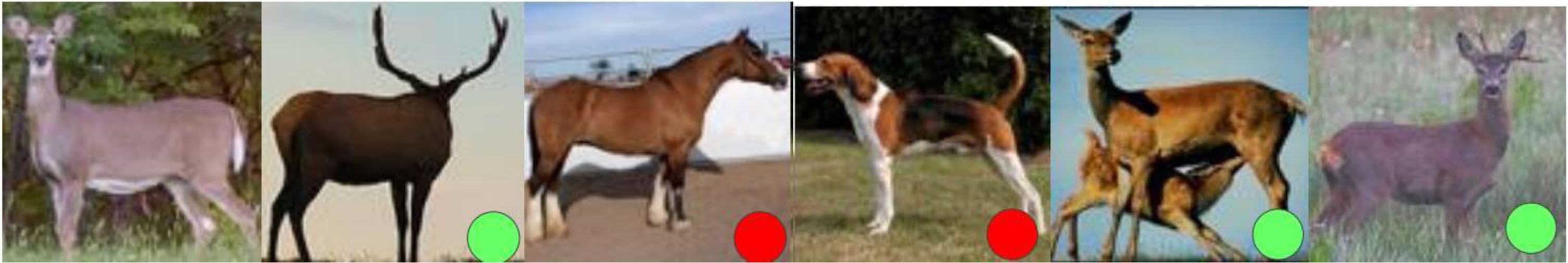
The semantic inconsistency between a sample and its nearest neighbors (STL-10 dataset).

To reduce the semantic inconsistency between a sample and its neighbors, we select k-nearest neighbors with high similarity. Next, a two-layer graph convolutional network (GCN) instead of a multilayer perceptron (MLP) is utilized. The connected nodes share the same semantic cluster in network-based classification when the adjacency matrix and Laplacian matrix are constructed [10].

Inspired by the MixUp algorithm [11], we use two different augmented views of an image to create a new image, increasing sample diversity and the number of positive samples. The contrastive loss is used to increase the similarity between positive sample pairs, which is consistent with the goal of feature learning, i.e., to learn the inherent feature representation of the augmented views. The main contributions of this paper are as follows:

(1) A new contrastive clustering method is proposed by leveraging an instance-level contrastive loss with mean square error (MSE) regularization and a cluster-level contrastive loss with cross-entropy regularization.

(2) A GCN is utilized as a feature projector to improve the semantic consistency of features. Samples whose similarity exceeds a predefined threshold are selected to reduce the potential for false positive sample pairs while constructing the adjacency matrix.

(3) Linear interpolation data augmentation is employed to increase sample diversity, reduce training difficulty, and improve the representation ability of the model.

The experimental results demonstrate that the GHDCC is an efficient deep contrastive clustering method.

2 Related work

2.1 Self-supervised representation and clustering

The earlier work of contrastive concept was proposed by Hadsell et al. in 2006 [12] to optimize the contrastive loss over pairs of samples. The classic contrastive learning method SimCLR [5] (a simple framework for contrastive learning of visual representation) was proposed by Hinton’s team. The two augmented views are considered a positive pair and are assumed to have a highly similar feature space, resulting in the same semantic cluster. The SimCLR learns the discriminative features by minimizing the normalized temperature-scaled cross-entropy loss (NT-Xent) to identify positive pairs across the dataset. This approach represented a breakthrough in self-supervised feature representation. Contrastive-based methods [13, 14] became popular after the introduction of the SimCLR method. Contrastive clustering (CC) [15] uses dual contrastive learning for deep clustering. It is an improved version of the SimCLR method and uses contrastive learning at the instance and cluster levels. The CC model jointly learns representations and cluster assignments in an end-to-end fashion. However, the CC performance is significantly influenced by the sample size. The model has a long runtime, and 8 threads are required for 160 GPU hours on the STL-10 dataset.

The SCAN method [8] is a two-stage method combining feature representation and cluster assignment. An image and its nearest neighbors are assumed to belong to the same semantic cluster. High-confidence samples are selected by thresholding the probability output provided by clustering. Pseudo-supervised learning is used to fine-tune the clustering parameters and the cluster assignments. The unsupervised visual representation algorithm (CoKe) [16] learns the relationship between instances based on the online constrained K-means. This online clustering method enables representation learning without interrupting encoder training. Another novel semantic clustering by partition confidence maximization (PICA) [17] was proposed. It learns representation features during training and the one-hot encoded cluster indices during testing by maximizing the global partition confidence of the clustering solution.

A nearest neighbor matching (NNM) clustering method [18] similar to SCAN was proposed to obtain semantic sample pairs with high confidence by optimizing the global and local consistent losses and class contrastive loss. This approach assesses the semantic sample relationships between local and global features, resulting in high clustering performance and low solution uncertainty. Neighborhood contrastive learning (NCL) learns discriminative features from the labeled data and has been used for novel class discovery (NCD) [19] using an unlabeled dataset. Semi-supervised NCL performs well and assumes that similar samples belong to the same class.

The Semantic Pseudo-labeling framework for Image ClustEring (SPICE) [1] divides the clustering network into a feature backbone and a cluster projector. Training is performed using contrastive learning and a pseudo-label algorithm, respectively. SPICE significantly reduces the gap between unsupervised and fully supervised classifications.

This paper proposed a self-supervised method, leveraging the pairwise similarity of positive/negative samples and analyzing the neighborhood using GCNs for unlabeled data. The method minimizes the occurrence of false positive pairs and has the benefits of neighborhood aggregation.

2.2 Data augmentation

Fan et al. [20] proposed a novel self-expert cloning technique to decouple robust representation learning using weak and strong augmentations. Random cropping is a type of weak augmentation. Strong augmentation refers to images with heavy distortion. The MixUp [11] method is a simple learning principle utilizing vicinal risk minimization (VRM). It trains a neural network on convex combinations of example pairs and their labels to reduce the risk of memorization and sensitivity to adversarial examples. Manifold MixUp [21], a variant of MixUp, uses semantic interpolations as additional training information to regularize the network for smoother decisions. The Co-Mixup method [22] maximizes saliency measurements to ensure super-modular diversity, significantly improving the cropping result.

The CutMix [23] method randomly crops a rectangular area and exchanges two rectangular patches to generate two augmented feature maps. The labels are mixed proportionally to the area of the patches. The network trained by the CutMix augmentations has a higher generalization ability and better object localization capability than the Cutout method. PatchUp [24] is another data augmentation method that crops patches to obtain the outputs in the hidden layer. Experimental results have shown that replacement-based methods provide higher recognition accuracy, and interpolation-based methods have higher robustness against attacks.

2.3 Graph convolutional network

A multilayer GCN was first proposed by Kipf and Welling [25] to classify graph-structured data with a few labels. The GCN is a variant of convolutional neural networks (CNNs) [26] with layer-wise propagation and contains a Laplacian matrix: $H^{(l + 1)} = σ (\hat{A} H^{(l)} W^{(l)}) .$

GCN-based classification [27] and face clustering [28] methods have made significant progress because the edges of the GCN encode the nodes’ similarities, providing additional information to improve model performance. Xie et al. [29] proposed an active and semi-supervised graph neural network (ASGNN) to deal with the scarcity of labeled graphs in graph classification. It is a semi-supervised active learning method that increases the number of pseudo-labeled graphs.

Another GCN-based semi-supervised method, GCN and semantic feature guidance for deep clustering (GFDC) [30] was used for deep clustering. A GCN with a Softmax output layer enables the discrimination of visual features for clustering. However, when the categories of two different datasets do not match completely, the clustering error increases significantly. Thus, we use positive and negative pair-based dual contrastive learning with GCN projectors for deep clustering in this study. It is an unsupervised method without any predefined annotations.

3 Methodology

We aim to group a set of images into several disjoint clusters without semantic labels. We propose the deep clustering method GHDCC, which consists of a feature extractor and a clustering projector. The parameters of the GHDCC are learned using the contrastive loss of sample discrimination as a pretext task. The goal of contrastive learning is to obtain the optimal feature representation by maximizing the similarity between positive sample pairs and minimizing the similarity between negative sample pairs. The proposed GHDCC can improve clustering performance and reduce the risk of generating degenerate solutions. The framework of the proposed GHDCC is shown in Fig. 2.

Fig. 2

The framework of the GHDCC model.

3.1 Problem formulation

For the given image dataset X = {x₁, x₂, . . . , x_N}, the goal of clustering is to allocate all samples into several disjoint clusters C = {C₁, C₂, ⋯ , C_K}, where N is the number of samples, and K is the number of predefined clusters. Contrastive clustering has two preprocessing steps. First, two of the five augmentation methods (random cropping, color jittering, grayscale, horizontal flip, and Gaussian blur) are randomly selected and are denoted as T^a and T^b. The original sample x_i generates two augmented samples $x_{i}^{a} = T^{a} (x_{i})$ and $x_{i}^{b} = T^{b} (x_{i})$ , while the third synthetic image is obtained using linear interpolation $x_{i}^{c} = λ x_{i}^{a} + (1 - λ) x_{i}^{b}$ , where parameter λ ∈ [0, 1]. The datasets are referred to as X^a, X^b, and X^c. A regular deep network (ResNet34) is used to extract useful and representative features from input samples using nonlinear mapping f : X^u → H^u, u ∈ {a, b, c}.

The GHDCC model consists of two GCNs that perform feature extraction. Each node contains information on itself and its neighbors in the latent space H [31]. The GCN, instead of a two-layer perceptron, guides the backbone network to learn the semantically discriminative features. The outputs of GCNs are allocated into several disjoint groups using the K-means algorithm.

3.2 Contrastive loss of GCN projectors

Instance-level projector GCN₁: GCN₁ is a two-layer perceptron (MLP) with a D-dimensional Softmax output. It projects features H and an adjacency matrix A into another latent space Z. $g_{1} : (H^{u}, A) \to Z^{u}, u \in {a, b, c} .$

Matrix A is a normalized adjacency matrix representing the semantic affinity between the nodes and their nearest neighbors using the cosine distance. The fine-tuned features Z^a and Z^b are expected to be more representative and useful for clustering. For a given feature $z_{i}^{a}$ , $(z_{i}^{a}, z_{i}^{b})$ is a positive pair, while $(z_{i}^{a}, {z_{j}}^{a})_{j \neq i}$ and $(z_{i}^{a}, {z_{j}}^{b})_{j \neq i}$ are 2*(batch_size -1) negative pairs. Similar to CC [15], the contrastive loss of the features is defined as follows:

$\begin{matrix} l_{i}^{a} = - log \\ \frac{exp (s (z_{i}^{a}, z_{i}^{b}) / τ_{1})}{\sum_{j = 1, j \neq i}^{N} exp (s (z_{i}^{a}, z_{j}^{a}) / τ_{1}) + \sum_{j = 1}^{N} exp (s (z_{i}^{a}, z_{j}^{b}) / τ_{1})} \end{matrix}$ (1) where $s (z_{i}, z_{j}) = \frac{z_{i} {z_{j}}^{T}}{∥ z_{i} ∥ ∥ z_{j} ∥}$ is the cosine similarity, and the temperature parameter τ₁ > 0. Equation (1) is a likelihood function; its numerator is related to the positive pair, and its denominator is the sum of the positive pair and the corresponding negative pair.

The instance-level contrastive loss is defined as:

$L_{ins} = \frac{1}{2 N} \sum_{i = 1}^{N} (l_{i}^{a} + l_{i}^{b})$ (2)

The similarity of the positive pair is maximized, and those of the negative pairs are minimized while minimizing L_ins. In addition, the MSE between $h_{i}^{a}$ and h_i^b ensures the transformation invariance of the feature pairs $(z_{i}^{a}, z_{i}^{b})$ .

$L_{mse} = \frac{1}{N} \sum_{i = 1}^{N} | | {h_{i}}^{a} - {h_{i}}^{b} | |_{2}^{2}$ (3)

Cluster-level projector GCN₂: GCN₂ is another two-layer network with the same structure as GCN₁, but they do not share the parameters. $g_{2} : (H^{u}, A) \to Y^{u}, u \in {a, b, c}$

Its output is the K-dimensional features Y_N×K, and K is the predefined number of clusters. Hard label clustering means that a sample is classified into a cluster. The row vector $y_{i}^{a}, i = 1, 2, \dots, N$ depicts the possibility of belonging to each cluster. The column vector $y_{k}^{a}, k = 1, 2, \dots, K$ is the probability distribution of N samples assigned to the k^th cluster. The positive pair output $(y_{k}^{a}, y_{k}^{b})$ is expected to be homogeneous, and the negative pair $(y_{k}^{a}, y_{l}^{a})$ is heterogeneous k ≠ l 1, 2, ⋯ , K. The contrastive loss is computed as:

$\begin{matrix} l_{k}^{a} = - log \\ \frac{exp (s (y_{k}^{a}, y_{k}^{b}) / τ_{2})}{\sum_{l = 1, l \neq k}^{K} exp (s (y_{k}^{a}, y_{l}^{a}) / τ_{2}) + \sum_{l = 1}^{K} exp (s (y_{k}^{a}, y_{l}^{b}) / τ_{2})} \end{matrix}$ (4) where the temperature parameter τ₂ > 0.

The cluster-level total contrastive loss is defined as:

$L_{cls} = \frac{1}{2 K} \sum_{k = 1}^{K} (l_{k}^{a} + l_{k}^{b}) + H (Y)$ (5)

$H (Y) = log (K) - \sum_{k = 1}^{K} \sum_{u = a, b} p (y_{k}^{u}) log p (y_{k}^{u})$ (6) where $p (y_{k}^{u}) = \frac{1}{N} \sum_{i = 1}^{N} y_{ik}^{u}$ represents the pseudo-label probability distribution in a given mini-batch. Minimizing H (Y) ensures the uniform distribution of $p (y_{k}^{u})$ and reduces the risk of degenerate clustering.

3.3 KL divergence in self-supervised learning

The linear interpolation ( ${\tilde{Y}}^{c} = λ Y^{a} + (1 - λ) Y^{b}$ ) results in an auxiliary distribution, where parameter 0 < λ < 1. Y^c is the output of GCN₂ for input X^c. The synthetic sample $x_{i}^{c}$ is more ambiguous than the augmented samples $x_{i}^{a}, {x_{i}}^{b}$ , enabling the backbone network to extract highly discriminative features in contrastive learning.

To this end, we optimize the Kullback-Leibler (KL) divergence between the two probability distributions to refine the representative ability of the backbone network. Thus, KL divergence loss is:

$KL ({\tilde{Y}}^{c} | | Y^{c}) = \frac{1}{NK} \sum_{i = 1}^{N} \sum_{k = 1}^{K} {\tilde{y}}_{ik}^{c} log (\frac{{\tilde{y}}_{ik}^{c}}{y_{ik}^{c}})$ (7)

Minimizing Equation (7) is equal to minimizing the cross-entropy (Equation (8)):

$L_{cross} = - \frac{1}{NK} \sum_{i = 1}^{N} \sum_{k = 1}^{K} {\tilde{y}}_{ik}^{c} log (y_{ik}^{c})$ (8) where N is the number of samples, and K is the number of predefined clusters. Y^c is the output of GCN₂ for input X^c. The auxiliary distribution ${\tilde{Y}}^{c} = λ Y^{a} + (1 - λ) Y^{b}$ is the linear interpolation

3.4 Adjacency matrix

Our backbone network ResNet34 is followed by a GCN; however, it is not an MLP as in CC [15] and SimCLR [5]. The feature and structural information is fed into the GCNs, resulting in high semantic similarity. Thus, our deep clustering method has the advantages of contrastive learning and a local neighborhood.

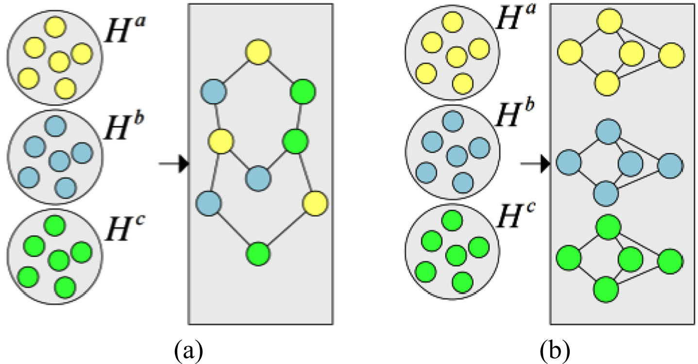
Two types of graphs are used. We concatenate three group features into $H = {[\begin{matrix} H^{a} \\ H^{b} \\ H^{c} \end{matrix}]}_{3 N \times D}$ and construct an adjacency matrix A according to H. First, an adjacency matrix A = (a_ij) _3N×3N is constructed by a cosine similarity with a pre-defined parameter τ, i.e., $a_{ij} = {\begin{matrix} s_{ij}, s_{ij} ⩾ τ \\ 0, s_{ij} < τ \end{matrix}$ , and $s_{ij} = \frac{h_{i}^{u_{1}} {(h_{j}^{u_{2}})}^{T}}{| | h_{i}^{u_{1}} | | | | h_{j}^{u_{2}} | |}$ , u₁, u₂ ∈ {a, b, c}. Next, a diagonal matrix D is built using $d_{i} = \sum_{j = 1}^{N} a_{ij}$ . The normalized adjacency matrix $\hat{A}$ is defined as $\hat{A} = D^{- \frac{1}{2}} (A + I) D^{- \frac{1}{2}}$ . This method is called as mixed graph in Fig. 3(a). The feature H and the normalized adjacency matrix $\hat{A}$ are fed into GCN₁ and GCN₂ for feature representation.

Fig. 3

Two types of topological graphs.

The other is called a concatenated graph in Fig. 3(b). Three smaller topological graphs and adjacency matrices are constructed according to {H^a, H^b, H^c} and concatenated to obtain a larger adjacency matrix. The mixed graph provides better clustering than the concatenated graph.

3.5 GHDCC algorithm

Equations (2), (3), (5), and (8) are combined. The total loss of the proposed GHDCC method is defined as:

$Loss = L_{ins} + λ_{1} L_{mse} + L_{cls} + λ_{2} L_{cross}$ (9) where parameters λ₁ > 0 and λ₂ > 0.

The training process of the clustering model GHDCC is summarized in Algorithm 1.

Algorithm 1: Training clustering model GHDCC
Inputs: Dataset X; Epochs E, batch size N, instance-level temperature τ₁, cluster-level temperature τ₂; Cluster number K; parameters λ₁ and λ₂.
Outputs: Clustering assignment
1. //initialization
Initialize network parameters; initialize adjacency matrix to zero matrix; obtain three augmentations X^a, X^b, X^c.
2. //training
for epoch = 1 to E do:
① obtain features H^u = f (X^u) , u = a, b, c, H = {H^a, H^b, H^c}
② obtain features Z^u = g₁ (H^u) by GCN₁; Y^u = g₂ (H^u) , u = a, b, c by GCN₂.
③ calculate instance-level loss using Equation (2) and the consistency using Equation (3);
④ calculate cluster-level loss using Equation (5) and the cross-entropy loss using Equation (8);
⑤ minimize the overall loss in Equation (9) to update f, g₁, g₂ network parameters;
⑥ save the GHDCC model;
end
3. // testing
for x in X:
① output feature z = f (x);
② output assignment Y by GCN₂;
③ evaluate clustering results
end

Complexity of the GHDCC algorithm is evaluated by the number of parameters and floating point operations(FLOPs). FLOPs can measure the computation complexity of a deep algorithm/model.

The GHDCC model is composed of ResNet34, two GCNs and K-means clustering. First, standard ResNet34 network has 34 convolutional layers without pooling and one fully-connected layer. Second, the parameters of two fully-connected networks are 2 * f_in * f_out that is far fewer than those of ResNet34. Third, time and space complexity of K-means clustering algorithm can be reduced to O(N), where N is the number of samples. Overall, the complexity of GHDCC algorithm is mainly the training of ResNet34.

Thus, the total number of parameters is about 200 w that is amount to 83MB. FLOPs is amount to about 3.4 G.

4 Experiments

4.1 Implementation details

The six image datasets used in the experiments are briefly described in Table 1.

Table 1
Information on the datasets used in this paper

Datasets Samples K Size

ImageNet-10 [32] 13000 10

ImageNet-Dogs 19500 15

Tiny-ImageNet 100000 200 32 × 32

CIFAR-10 [33] 60000 10 32 × 32

CIFAR100-20 60000 20 32 × 32

STL-10 [34] 13000 10 96 × 96

Datasets	Samples	K	Size
ImageNet-10 [32]	13000	10
ImageNet-Dogs	19500	15
Tiny-ImageNet	100000	200	32 × 32
CIFAR-10 [33]	60000	10	32 × 32
CIFAR100-20	60000	20	32 × 32
STL-10 [34]	13000	10	96 × 96

We resize all input images to 64×64; the batch size is 128, and the learning rate is 2e - 4. The GHDCC framework contains a ResNet34 and two GCNs. ResNet34 reduces the inputs to 128-dimensional features. GCN₁ and GCN₂ perform feature extraction, and the outputs are 128-dimensional and K-dimensional. Adaptive moment estimation (Adam) [35] is used as the optimizer. The GHDCC model is trained using 500 epochs. The linear interpolation parameter is λ = 0.7. The trade-off parameters are λ₁ = λ₂ = 0.5, and the temperature parameters are τ₁ = 0.5 and τ₁ = 1. The GHDCC model is built using Python 3.7 under the Pytorch framework; and the experiments are carried out on Nvidia RTX 3060 GPU.

The GHDCC model is evaluated using the clustering accuracy (ACC) [36], normalized mutual information (NMI) [37], and the adjusted Rand index (ARI) [38]. The larger the value of these indicators, the better the clustering performance of the model is.

4.2 Comparison experiments

Comparison experiments were conducted. CC and GCC are two competitive comparators. The comparison results with other clustering methods are listed in Table 2. The accuracies are obtained by running the original codes in our experimental environment. The best results are shown in bold, and the second-best results are underlined. The clustering results indicate that the GHDCC algorithm provides good performance. The SPICE method provides the highest clustering accuracy of 0.959, 0.926, and 0.938 on the ImageNet-10, CIFAR-10, and STL-10 datasets, respectively, outperforming the proposed GHDCC algorithm by a large margin. The reason is maybe the limited hardware and the smaller image size.

Table 2
Comparison of the accuracies of the GHDCC and several baseline methods

Methods References ImageNet-10 ImageNet-Dogs Tiny-ImageNet CIFAR-10 CIFAR100-20 STL-10

K-means [39] 0.238 0.103 0.028 0.206 0.131 0.210

DEC [40] ICML2016 0.393 0.202 0.084 0.244* 0.174 0.359*

DAC [41] ICCV2017 0.527* 0.275* – 0.522* 0.238* 0.470*

PICA [17] CVPR2020 0.870* 0.352* 0.098* 0.696* 0.337* 0.713*

GCC [9] ICCV2021 0.901* 0.526* 0.138* 0.856* 0.472* 0.788*

CC [15] (1000) AAAI2021 0.893* 0.429* 0.140* 0.790* 0.429* 0.850*

CC (500) 0.826 0.269 0.135 0.692 0.370 0.706

OURS 0.913 0.346 0.240 0.689 0.396 0.711

Methods	References	ImageNet-10	ImageNet-Dogs	Tiny-ImageNet	CIFAR-10	CIFAR100-20	STL-10
K-means [39]		0.238	0.103	0.028	0.206	0.131	0.210
DEC [40]	ICML2016	0.393	0.202	0.084	0.244*	0.174	0.359*
DAC [41]	ICCV2017	0.527*	0.275*	–	0.522*	0.238*	0.470*
PICA [17]	CVPR2020	0.870*	0.352*	0.098*	0.696*	0.337*	0.713*
GCC [9]	ICCV2021	0.901*	0.526*	0.138*	0.856*	0.472*	0.788*
CC [15] (1000)	AAAI2021	0.893*	0.429*	0.140*	0.790*	0.429*	0.850*
CC (500)		0.826	0.269	0.135	0.692	0.370	0.706
OURS		0.913	0.346	0.240	0.689	0.396	0.711

Note: “*” denotes the clustering accuracy obtained in a previous study, “-” denotes no value available. The best results of the last two rows are shown in bold, and the second-best results are underlined.

We assessed the training cost of the backbone network and the hardware requirements of CC (the input image is 224×224, the batch size is 256, and there are 1000 training epochs. The shortest running time on the GPU is 20 hours, and the longest is 160 hours). The similar situation is for the GCC. Due to the limitation of hardware, we retrained the ResNet34 using 64×64 input images and the other default training parameters of CC. We report the clustering accuracy in 500 training epochs (CC (500)) and then train the GHDCC model. The results are listed in Table 2.

The GCC and GHDCC are two variants of the CC method. They both use the k-nearest neighbors to increase the number of positive sample pairs and improve clustering performance. As shown in Table 2, our method outperforms the GCC and CC (1000) by 1.2% and 2% on ImageNet-10 and by 10.2% and 10% on Image-dogs, respectively. However, it performs the worst on the other four datasets. The reason is that the batch size and input image size of the GHDCC are significantly smaller than those of the GCC and CC (1000).

The GHDCC significantly outperforms CC (500) by a large margin, except on CIFAR-10. The clustering accuracy of GHDCC is 10.5% higher than that of CC (500) on Tiny-ImageNet. Furthermore, the GHDCC shows comparable performance to most state-of-the-art methods.

As shown in Table 3, the three evaluation indicators are consistent, indicating reliable clustering results. The GCN₁ uses t-distributed stochastic neighbor embedding (t-SNE) [42] (Fig. 4). Different colors represent different clusters. It is observed that the distance between the clusters increases during iterative optimization.

Table 3

Clustering performances of the GHDCC on six datasets

Datasets	ACC	NMI	ARI
ImageNet-10	0.913	0.890	0.840
ImageNet-Dogs	0.346	0.381	0.200
Tiny-ImageNet	0.240	0.420	0.137
CIFAR-10	0.689	0.602	0.525
CIFAR100-20	0.396	0.391	0.240
STL-10	0.711	0.597	0.517

Fig. 4

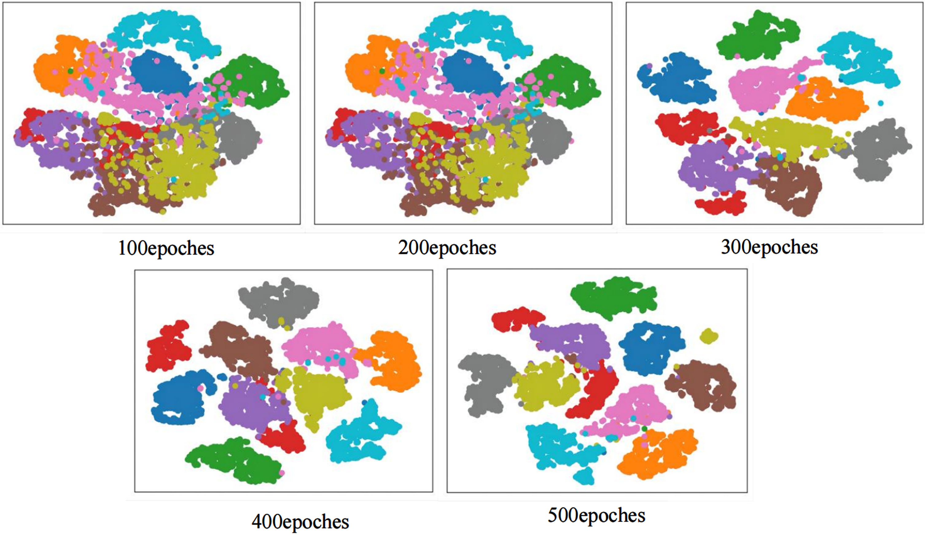
Visualization of the GCN₁ features after training GHDCC on ImageNet-10.

4.3 Ablation study results

Three ablation studies were conducted to verify the performance of the components of the proposed method.

First, the impact of the adjacency matrix (Section 3.3) on the clustering results was tested on ImageNet-10. The mixed graph pattern provides 0.913 clustering accuracy, and the concatenated graph has an accuracy of 0.812. The comparison indicates that the mixed graph can extract higher discriminative features.

Second, the two-layer MLP was compared with the GCN; both were implemented as projectors after ResNet34. The features are visualized in Fig. 5. The first column in Fig. 5 shows the features extracted by ResNet34 and ResNet34 + MLP. The second column shows the features extracted by ResNet34 and ResNet34 + GCN.

Fig. 5

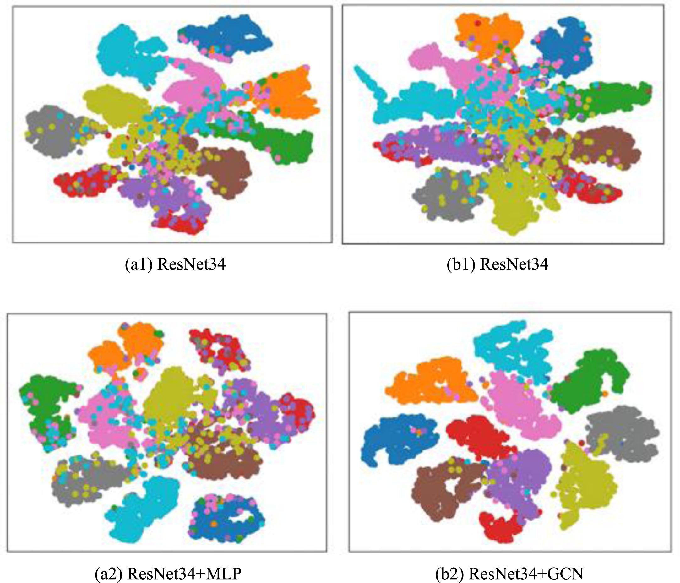
Visualization of the features obtained from projectors MLP and GCN on ImageNet-10.

The results indicate that the boundary between the clusters is better defined in Fig. 5 (b2) than in Fig. 5 (a2), and the samples in the clusters are more compact. In addition, the clusters in Fig. 5 (b1) are not as well defined as those in Fig. 5 (a1). Thus, the GCN better describes the relationship between the samples and minimizes solution uncertainty.

Third, linear interpolation data augmentation was used to increase the sample size. The parameter λ in the linear interpolation substantially influences the quality of the data set and the experimental results. Therefore, we tested different λ values on several datasets. The results of ImageNet-Dogs are shown in Fig. 6. The optimal clustering accuracy is λ = 0.7.

Fig. 6

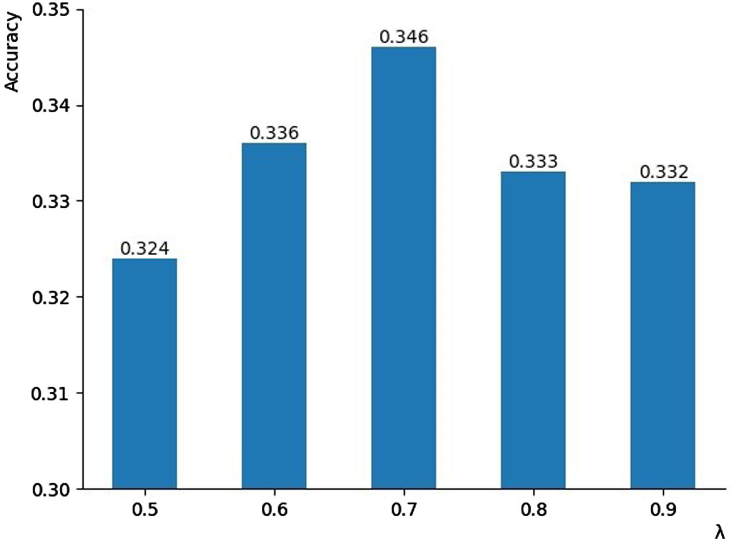
The effect of the λ values on the clustering accuracy on ImageNet-Dogs.

The clustering accuracies obtained from the ablation experiments are listed in Table 4. The projector GCN significantly improves the clustering accuracy of the GHDCC method. Linear interpolation data augmentation also improves the performance of the GHDCC method.

Table 4

Clustering accuracies of the GHDCC components in the ablation experiments

Datasets	w/o GCN	w/o linear interpolation	GHDCC
ImageNet-10	0.621	0.899	0.913
ImageNet-Dogs	0.242	0.343	0.346
Tiny-ImageNet	0.094	0.230	0.240
CIFAR-10	0.677	0.683	0.689
CIFAR100-20	0.356	0.367	0.396
STL-10	0.620	0.651	0.711

The confusion matrices on ImageNet-10 are shown in Fig. 7. The diagonal elements represent the number of correctly classified samples. A brighter yellow color indicates that more samples are correctly classified. Replacing the MLP with the GCN, i.e., Fig. 7(b) vs. Fig. 7(a) significantly improves the clustering accuracy. The accuracy of the GHDCC algorithm is 0.913 when linear interpolation data augmentation is used (Fig. 7(c)).

Fig. 7

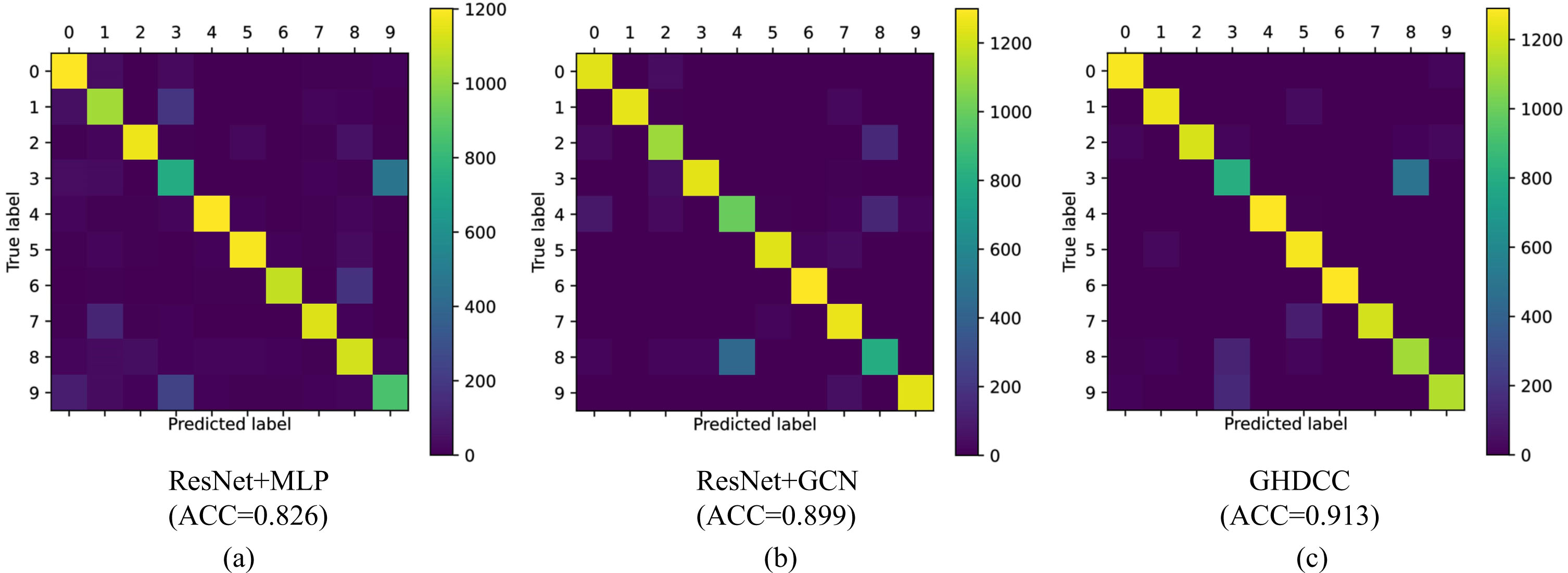
Confusion matrix of the GHDCC on ImageNet-10.

5 Conclusion

The paper proposed a self-supervised learning approach called GHDCC for image clustering. It uses contrastive clustering to learn more discriminative features. GHDCC utilizes a GCN and a convex combination of data to prevent false positive samples and improve the extraction of semantic features. The experimental results demonstrated that GHDCC achieved improved clustering performance on six baseline datasets and outperformed most state-of-the-art clustering methods evaluated in this study. The ablation study results indicated that every component of the GHDCC model contributed to improving the clustering performance.

However, the clustering performance of GHDCC was limited by the small image size, affecting the pixel-level information. We plan to improve the GHDCC’s performance by using a larger image size and a higher-capacity GPU. Another objective is to use the GHDCC model for image inpainting via Features Fusion and Two-steps Inpainting algorithm (FFTI) [43] in the Expectation-Maximization (EM) framework.

References

Niu

, Shan

H.M.

and Wang

, SPICE: semantic pseudo-labeling for image clustering, IEEE Trans on Image Processing (2022), 1–15.

Wang

C.Z.

, Bai

X.Y.

and Du

J.L.

, Image diffusion interfaces for unsupervised clustering algorithm, Computer Science 47(5) (2020), 149–153.

Liu

A.T.

, Yang

S.H.

, Chi

P.H.

, et al., Mockingjay: unsupervised speech representation learning with deep bidirectional transformer encoders, in Proc. 45th Int. Conf. on Acoustics, Speech and Signal Processing, Barcelona, Spanish, 2020, pp. 6419–6423.

Ravanelli

, Zhong

J.Y.

, Pascual

, et al., Multi-task self-supervised learning for robust speech recognition, in Proc. 45th Int. Conf. on Acoustics, Speech and Signal Processing, Barcelona, Spanish, 2020, pp. 6989–6993.

Chen

, Kornblith

, Norouzi

and Hinton

, A simple framework for contrastive learning of visual representations, in Proc. 37th Int. Conf. Machine Learning, 2020, pp. 1597–1607.

Algayres

, Zaiem

M.S.

, Sagot

, et al., Evaluating the reliability of acoustic speech embeddings, presented at the 21st Annual Conf. of the Int. Speech Communication Association, Shanghai, China, 2020.

Sohn

, Improved deep metric learning with multi-class n-pair loss objective, presented at Advances in neural information processing systems, 2016, pp. 1857–1865.

Van Gansbeke

, Vandenhende

, Georgoulis

, et al., Scan: Learning to classify images without labels, presented at the 16th European Conf. Computer Vision, Glasgow, UK, 2020, pp. 268–285.

Zhong

H.S.

, Wu

J.L.

, Chen

, et al., Graph Contrastive Clustering, presented at the 2021 IEEE/CVF Int. Conf. Computer Vision, Montreal, QC, Canada, Oct. 2021, pp. 9204–9213.

10.

Weston

, Ratle

, Mobahi

and Collobert

, Deep learning via semi-supervised embedding. In Neural Networks: Tricks of the Trade, 2012, pp. 639–655.

11.

Zhang

, Cisse

and Dauphin

Y.N.

, Mixup: Beyond empirical risk minimization, in Proc. 6th Int. Conf. on Learning Representations, Vancouver, BC, Canada, 2018.

12.

Hadsell

, Chopra

and LeCun

, Dimensionality reduction by learning an invariant mapping. presented at the, 2006 IEEE/CVF Conf. Computer Vision and Pattern Recognition 2 (2006), 1735–1742.

13.

Saeed

, Grangier

and Zeghidour

, Contrastive learning of general-purpose audio representations, in Proc. 46th Int. Conf. on Acoustics, Speech and Signal Processing, Toronto, Canada, 2021, pp. 3875–3879.

14.

Yao

Y.Z.

, Sun

Z.R.

, Zhang

C.Y.

, et al., Jo-SRC: A contrastive approach for combating noisy labels, Presented at the 2021 IEEE/CVF Conf. on Computer Vision and Pattern Recognition, Online, 2021, pp. 5192–5201.

15.

Y.F.

, Hu

, Liu

Z.T.

, et al., Contrastive clustering, presented at the 35th AAAI Conf. Artificial Intelligence, New York, USA, 2021, pp. 8547–8555.

16.

Qian

, Xu

Y.H.

, Hu

J.H.

, et al., Unsupervised visual representation learning by online constrained k-means, Presented at the 2021 IEEE/CVF Conf. on Computer Vision and Pattern Recognition, Online, 2021.

17.

Huang

, Gong

and Zhu

, Deep semantic clustering by partition confidence maximisation, Presented at the 2020 IEEE/CVF Conf. on Computer Vision and Pattern Recognition, 2020.

18.

Dang

, Deng

, Yang

, et al., Nearest neighbor matching for deep clustering, Presented at the IEEE/CVF Conf. on Computer Vision and Pattern Recognition, Online, 2021, pp. 13693–13702.

19.

Zhong

, Fini

, Roy

, et al., Neighborhood contrastive learning for novel class discovery, Presented at the IEEE/CVF Conf. on Computer Vision and Pattern Recognition, Online, 2021, pp. 10867–10875.

20.

Fan

L.X.

, Wang

G.Z.

, Huang

D.A.

, et al., Secant: self-expert cloning for zero-shot generalization of visual policies. In Proc. 33rd Int. Conf. Machine Learning, 2021.

21.

Verma

, Lamb

, Beckham

, et al., Manifold mixup: Better representations by interpolating hidden states, in Proc. of the 36th Int. Conf. on Machine Learning, Long Beach, California, USA, 2019, pp. 6438–6447.

22.

Kim

J.H.

, Choo

, Jeong

, et al., Co-mixup: Saliency guided joint mixup with supermodular diversity, in Proc. of the 9th Int. Conf. on Learning Representations, Online, 2021.

23.

Yun

, Han

, Oh

S.J.

, et al., Cutmix: Regularization strategy to train strong classifiers with localizable features, Presented at the 2019 IEEE/CVF Int. Conf. Computer Vision, Seoul, Republic of Korea, 2019, pp. 6023–6032.

24.

Faramarzi

, Amini

, Badrinaaraayanan

, et al., Patchup: A regularization technique for convolutional neural networks, arXiv preprint arXiv:2006.07794, 2020.

25.

Kipf

T.N.

and Welling

, Semi-Supervised classification with graph convolutional networks, in Proc. 5th Int. Conf. Learning Representations, 2017.

26.

Z.W.

, Pan

S.R.

, Chen

F.W.

, et al., A comprehensive survey on graph neural networks, IEEE Trans on Neural Networks and Learning Systems 32(1) (2020), 4–24.

27.

Z.R.

, Ye

Z.L.

and Zhao

H.X.

, A graph convolutional neural network method based on mixed feature modeling, Computer Application (2020), 1–13.

28.

Wang

W.B.

and Luo

H.L.

, Complete graph face clustering based on graph convolutional neural network, Computer Science 48(11A2) (2021), 275–277.

29.

Xie

, Lv

and Qian

, Active and semi-supervised graph neural networks for graph classification, IEEE Trans. on Big Data, 2022.

30.

Chen

J.F.

, Han

, Meng

X.J.

, et al., Graph convolutional network combined with semantic feature guidance for deep clustering, Tsinghua Science Technol 27(5) (2022), 855–868.

31.

Kipf

T.N.

and Welling

, Variational graph autoencoders, in Pro. of the Conf. and Workshop on Neural Information Processing Systems, Barcelona, Spain, 2016.

32.

Deng

, Dong

, Socher

, et al., A large-scale hierarchical image database, in Proc. of the 10th IEEE Conf. on Computer Vision and Pattern Recognition, Miami, Florida, USA, 2009.

33.

Krizhevsky

and Hinton

, Learning multiple layers of features from tiny images, Handbook of Systemic Autoimmune Diseases 1(4) (2009).

34.

Coates

, Lee

H.L.

and Ng

A.Y.

, An analysis of single-layer networks in unsupervised feature learning, in Proc. of the 14th Int. Conf. on Artificial Intelligence and Statistics, 2011, pp. 215–223.

35.

Kingma

D.P.

and Ba

, Adam:Amethod for stochastic optimization, in Proc. 3rd Int. Conf. Learning Representations, San Diego, USA, 2015, pp. 1–15.

36.

and Ding

, The relationships among various nonnegative matrix factorization methods for clustering, presented at the 6th Int. Conf. Data Mining, Hong Kong, China, 2006, pp. 362–371.

37.

Strehl

and Ghosh

, Cluster ensembles-A knowledge reuse framework for combining multiple partitions, J. Mach. Learn. Res. 3 (2003), 583–617.

38.

Hubert

and Arabie

, Comparing partitions, J. Classifier. 2(1) (1985), 193–218.

39.

MacQueen

, Some methods for classification and analysis of multivariate observations, in Proc. 5th Berkeley Symp. Mathematical Statistics and Probability, Berkeley, USA, 1967, pp. 281–297.

40.

Xie

J.Y.

, Girshick

and Farhadi

, Unsupervised deep embedding for clustering analysis, in Proc. 33rd Int. Conf. Machine Learning, New York, USA, 2016, pp. 478–487.

41.

Chang

J.L.

, Wang

L.F.

, Meng

G.F.

, et al., Deep adaptive image clustering, in Proc. of the 31st IEEE Int. Conf. on Computer Vision, Venice, Italy, 2017, pp. 5879–5887.

42.

van der Maaten

and Hinton

, Visualizing data using t-SNE, J. Mach. Learn. Res. 9(86) (2008), 2579–2605.

43.

Chen

Y.T.

, Xia

R.L.

, Zou

and Yang

, FFTI: Image Inpainting Algorithm via Features Fusion and Two-Steps Inpainting, J. Vis. Commun. Image R. 91 (2023), 103776–103780.

A self-supervised learning of semantic feature consistency for image clustering

Abstract

Keywords

1 Introduction

2.1 Self-supervised representation and clustering

2.2 Data augmentation

2.3 Graph convolutional network

3 Methodology

3.2 Contrastive loss of GCN projectors

4.1 Implementation details

Table 1 Information on the datasets used in this paper Datasets Samples K Size ImageNet-10 [32] 13000 10 ImageNet-Dogs 19500 15 Tiny-ImageNet 100000 200 32 × 32 CIFAR-10 [33] 60000 10 32 × 32 CIFAR100-20 60000 20 32 × 32 STL-10 [34] 13000 10 96 × 96

References

Table 1
Information on the datasets used in this paper

Datasets Samples K Size

ImageNet-10 [32] 13000 10

ImageNet-Dogs 19500 15

Tiny-ImageNet 100000 200 32 × 32

CIFAR-10 [33] 60000 10 32 × 32

CIFAR100-20 60000 20 32 × 32

STL-10 [34] 13000 10 96 × 96