
Abstract
Despite the significant improvements in the detection and diagnosis of plant diseases at an early stage facilitated by deep learning technology, there are challenges associated with the generalization performance of deep learning models. These problems from the differences between in-field and in-lab data, as well as the heterogeneity of training and prediction data features. In the case of tomato leaf diseases, the PlantVillage dataset is widely used and has already demonstrated accuracy of more than 99%. However, using trained model based on this dataset to predict in-field data results in low accuracy due to domain differences and heterogeneous features. In this paper, we propose a domain adaptation method based on CycleGAN to solve this problem, followed by a preprocessing technique that utilizes both the OpenCV module and a segmentation model based on U-Net for the best generalization performance. The classification accuracy is evaluated by applying the DenseNet121 model trained on the PlantVillage dataset to the images generated by CycleGAN. Our results demonstrate, with an F1-score of 95.6%, that our domain adaptation method between the two domains is effective in mitigating the effect of domain shift.
Keywords
Introduction
Many countries have recently adopted smart agriculture technologies to promote agricultural modernization, such as the Internet of Things, artificial intelligence, and cloud computing. Meanwhile, tomatoes are the most widely produced and consumed vegetable worldwide whose production continues to increase annually. In this context, the greatest concern in tomato production is disease prediction and diagnosis.
The main causes of tomato production and quality degradation are crop diseases caused by changes in environmental factors [1]. Leaf mold is a disease that causes tomato leaves to turn yellow and wither and particularly tends to spread to upper leaves, causing significant damage to tomato production. Thus, predicting and detecting diseases in tomatoes is critical. Computer vision technology a branch of artificial intelligence aimed at teaching computers to interpret and interact with the visual world is widely used for such tasks.
Computer vision approaches based on deep learning technology are rapidly evolving in the fields of object detection [2], image classification [3], autonomous vehicles [4], and medicine [5]. Specifically, deep learning technology is being used in smart agriculture to detect and classify crop diseases. Among deep learning technologies, convolutional neural networks (CNNs) [6] such as the 2012 AlexNet [7] and more recent EfficientNet [8] outperform others with regard to effectively recognizing image features via convolution operations.
Deep learning models have been grafted with pre-trained models including ResNet50 [9], Inception V3 [10], and Xception [11] to predict tomato leaf disease. In one study, AlexNet [12] and SqueezeNet [13] models predicted a total of 10 diseases: late blight, early blight, bacterial spots, leaf mold, septoria spots, target spots, spider mites, yellow leaf curl virus, health, and virus. The prediction accuracies were 95.65% and 94.3%, respectively, showing the possibility of advancing disease detection in a green-house environment with an automated system. Kumar and Vani predicted outcomes for PlantVillage datasets using LeNet, ResNet50, and Xception, Visual Geometry Group 16 (VGG16) models [14]. These models showed high accuracies, i.e., 96.27%, 98.65%, 98. 13%, and 99.25%, respectively. Nandhini and Ashokkuma proposed new models for six diseases: healthy, late blight, bacterial spots, septoria, leaf spots, and mosaic viruses. In the both the VGG16 and Concept V3 approaches, the CNN complexity of the model was optimized using the improved crossover-based monarch butterfly optimization algorithm [15], reaching accuracy values of 99.98% and 99.94%, respectively.
Especially, the dataset is the most important component of the CNN model with regard to learning and prediction. In general, the crop images gathered from various farms are not standardized. There are also differences in the latent similarities (such as background, brightness, and saturation) in each crop’s regions of interest (ROIs). A CNN model with a performance of 99.9% or higher was introduced for recently released images of tomato leaf disease [16]. However, domain shifting occurs when predicting images are collected from farms in different environments, resulting in poor prediction performance. Several studies applied transfer learning or domain adaptation techniques to minimize these issues [17].
Many excellent models have been developed for predicting tomato leaf diseases based on the PlantVillage dataset, with some models achieving up to 99.5% accuracy. However, data collected in the field differ from that in the PlantVillage dataset, predicting field data without transfer learning results in poor performance owing to the domain shift phenomenon. Furthermore, compared to healthy leaf images, the disease image data collected in the field are relatively insufficient, resulting in a poor learning performance. To solve these issues, the generalized adversarial network (GAN) has been used to improve images for diseases with insufficient data. LeafGAN [18], CGAN [19], and arGAN are deep learning algorithms for data augmentation based on CycleGAN [20]. The LeafGAN is a GAN-based data augmentation method using label-free leaf segmentation (LFLSeg) module. The generated synthetic images are effective in improving the accuracy of plant disease diagnosis models and the LeafGAN model is computationally efficient with fewer parameters than other GAN-based approaches. Chen’s proposed algorithm also improved disease classification performance by enhancing an existing image [21]. Other studies have shown proper transformations between domains while retaining existing features. Long proposed a method for aligning the extracted features from task-specific networks across source and target domains by minimizing distance metrics such as the maximum mean discrepancy [22]. Hoffman proposed a cycle consistent adversarial domain adaptation algorithm for combining features and pixel-level adaptations into a single architecture and provided state-of-the-art results for a variety of visual adaptation tasks [23]. Pixel-level adaptation is the process of learning a mapping or transformation function between two domains to align the source and target distributions in a raw pixel space. Studies have shown that the use of the pixel-level cycle loss outperforms feature-level adversarial discriminatory domain adaptation [24].
To develop and evaluate deep learning models for real-world applications, such as field deployment, it is necessary to enhance the generalization performance, which is degraded due to the heterogeneity between in-lab and in-field environment dataset. Various approaches, including data preprocessing, domain adaptation, augmented data generation, and transfer learning, can be used to address these issues. Preprocessing of data improves data consistency, while domain adaptation bridges the gap between laboratory and field data. The lack of field data is supplemented by augmented data generation, and transfer learning employs previously trained models to extract field-appropriate features. In this context, the main contributions of this paper are: Initially, we propose a preprocessing strategy for image data to address the generalization performance issues resulting from the heterogeneity between the two domains. The second is to develop a lightweight CycleGAN model suitable for field applications, enabling the generation of multi-class images using a single model. Specifically, we applied PlantVillage and field collected data as training images and perform domain adaptation using CycleGAN. Additionally, two CycleGAN models were utilized to conduct the experiments. The first one was the Multi CycleGAN without classification adversarial loss, while the other was the Single CycleGAN with this loss. To assess the impact of the proposed preprocessing technique, we performed disease prediction using pre-trained DenseNet121 [25] with images generated by each CycleGAN.
The remainder of this paper is organized as follows. Section 2 presents a method for preprocessing the training images and constructing CycleGAN for domain adaptation, as well as evaluating the classification performance of the generated images. Section 3 presents the evaluation indicators and results of the learning model. Section 4 presents the conclusions from the proposed method.
Materials and methods
In this section, we present the in-lab and in-field environment datasets along with the domain adaptation method. Figure 1 depicts the overall process flow of the proposed method. In the first stage, we propose a method for standardizing the geometric properties of in-lab and field data. These images are then used as training data for the CycleGAN model in stage 2. In stage 3, the classification performance of the images generated by CycleGAN is evaluated using the DenseNet model. It is also utilized during the second stage of CycleGAN’s training to compute the loss for each disease class.
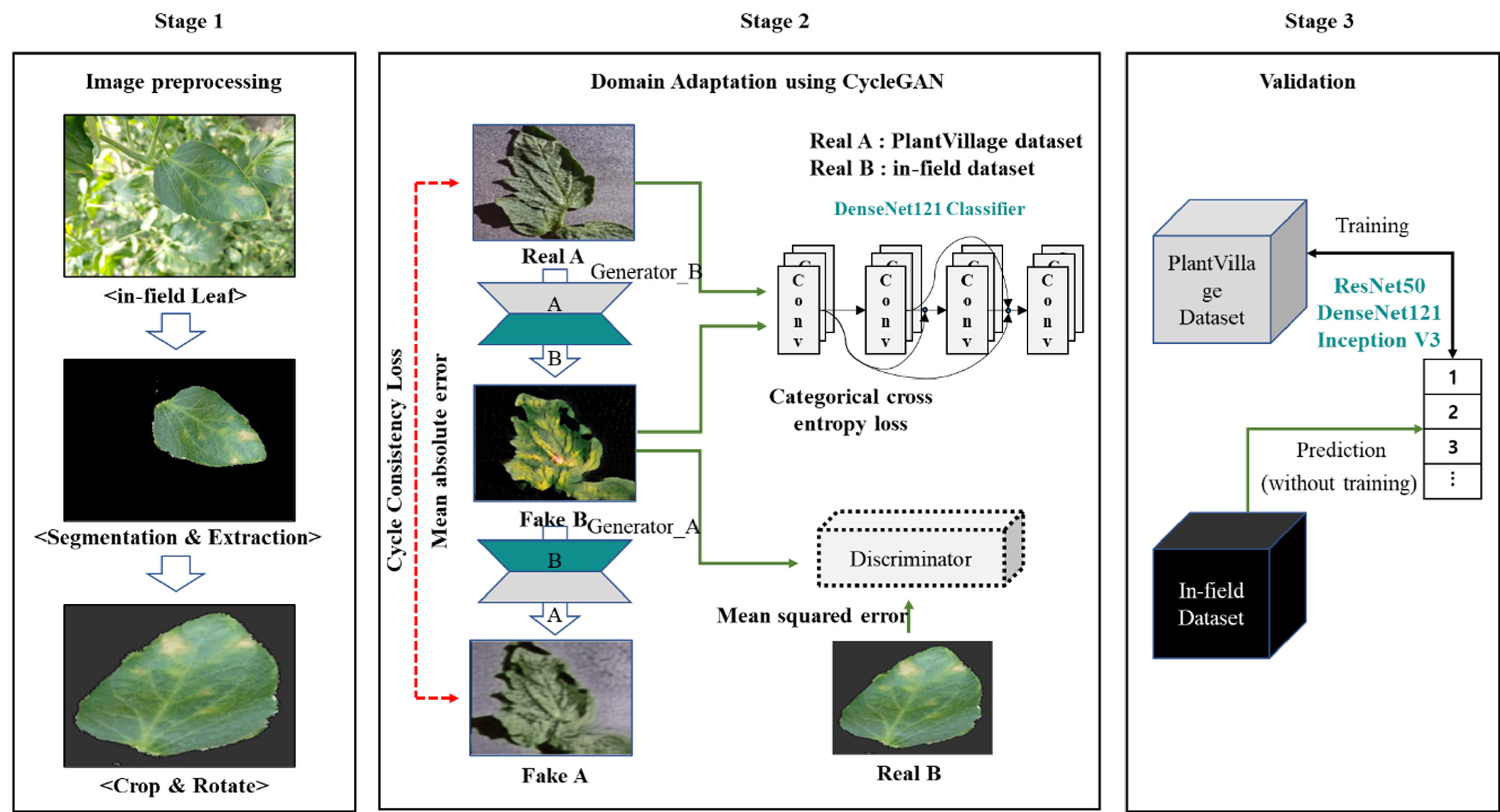
The overall workflow of the proposed methodology in this study is as follows: stage 1) image preprocessing, stage 2) Domain adaptation using CycleGAN, stage 3) validation using DenseNet121.
We used the publicly available tomato PlantVillage dataset for the proposed method [26]. The PlantVillage dataset contains images of 16,000 tomato leaves divided into ten classes. Nine of the ten classes correspond to disease images, whereas the remaining class corresponds to healthy images. The Ministry of Science and ICT funded the field data collection in this study. The data was built with the help of the Korea Intelligent Information Society Promotion Agency (AI Hub) and “Facility Crop Disease Diagnostic Image.” The tomato images provided by the AI hub were divided into three classes, with one class including healthy leaves. As some overlapping images or fruit images were mixed with the leaf images, only 600 images were used in this study. In addition, because it was impossible to expose the AI hub images, some images in this study were obtained from the Internet. “Local images” refers to a downloaded images and AI hub images. Table 1 displays the detailed information from the PlantVillage and AI hub datasets used in this study. Only three classes were used for the data balancing (including the class comprising healthy leaves).
Image distribution of the tomato leaf dataset
Image distribution of the tomato leaf dataset
Figure 2 depicts the heterogeneous features, in particular the latent similarities between the PlantVillage and local image domains, such as differences in background and brightness. These features are observable in both in-lab and in-field environment data as significant factors.
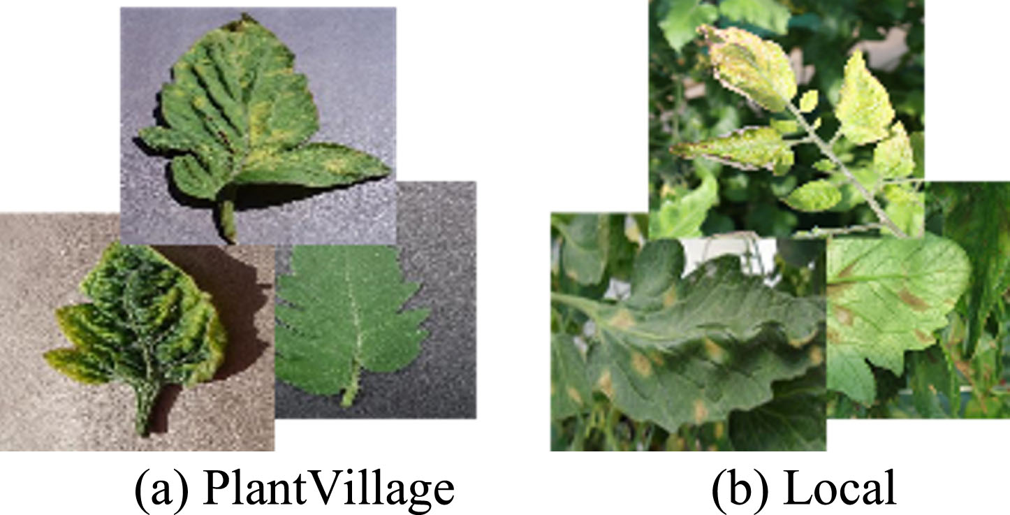
An example of two different domains. These two domains exhibit significant differences in background, color, and lighting.
Although the disparity in color and background is consistent with the application purpose of CycleGAN, the differences in shape, specifically in the region of interest without the background, negatively impact the generalization performance during CycleGAN training. To overcome this limitation, we employed image preprocessing techniques to align the geometric features of the two domains, ensuring they resemble the in-lab environment. This approach is beneficial for practical applications as it allows for standardization of in-field data to match the characteristics of in-lab data. The procedure for image preprocessing consisted of two stages. In the initial phase of the segmentation procedure, the U-Net model was utilized to distinguish the region of interest from the background. After the ROI region was extracted, it was cropped and rotated to match the shape of the PlantVillage dataset in the second step.
To properly segment the desired leaves in the CycleGAN model, annotated training images are necessary. In this study, Photoshop was utilized to create annotations for around 400 high-resolution images, which represents roughly 70% of our local dataset. Next, the segmented images were converted from BGR to grayscale using OpenCV. Then, they were transformed to binary mask images, in which the ROIs area is set to 1 and the background area is set to 0.
Segmentation
In this study, two segmentation models were applied. grabCut is the first applied module that does not require training. Using boundary data, the grabCut module separates objects from the background. It employs the Graph Cut algorithm during the iterative optimization phase to more precisely estimate the boundaries between objects and the background. As depicted in Fig. 3, the second model is based on the U-Net architecture. The encoder network was created using ResNet50, which is a pre-trained model to extract features from the original image. On the other hand, the decoder network generates a mask image corresponding to a division map based on the feature map extracted by the encoder. To prevent gradation from disappearing during decoding, a net block was applied to the rear of the convolution layer. Additionally, ResNet blocks were used to create two 3x3 convolutional layers without lowering the resolution of the feature map. To enhance the performance of the model, batch normalization and a leaky rectified linear unit (Leaky ReLU) activation function were applied to the bottom of the convolution layer.
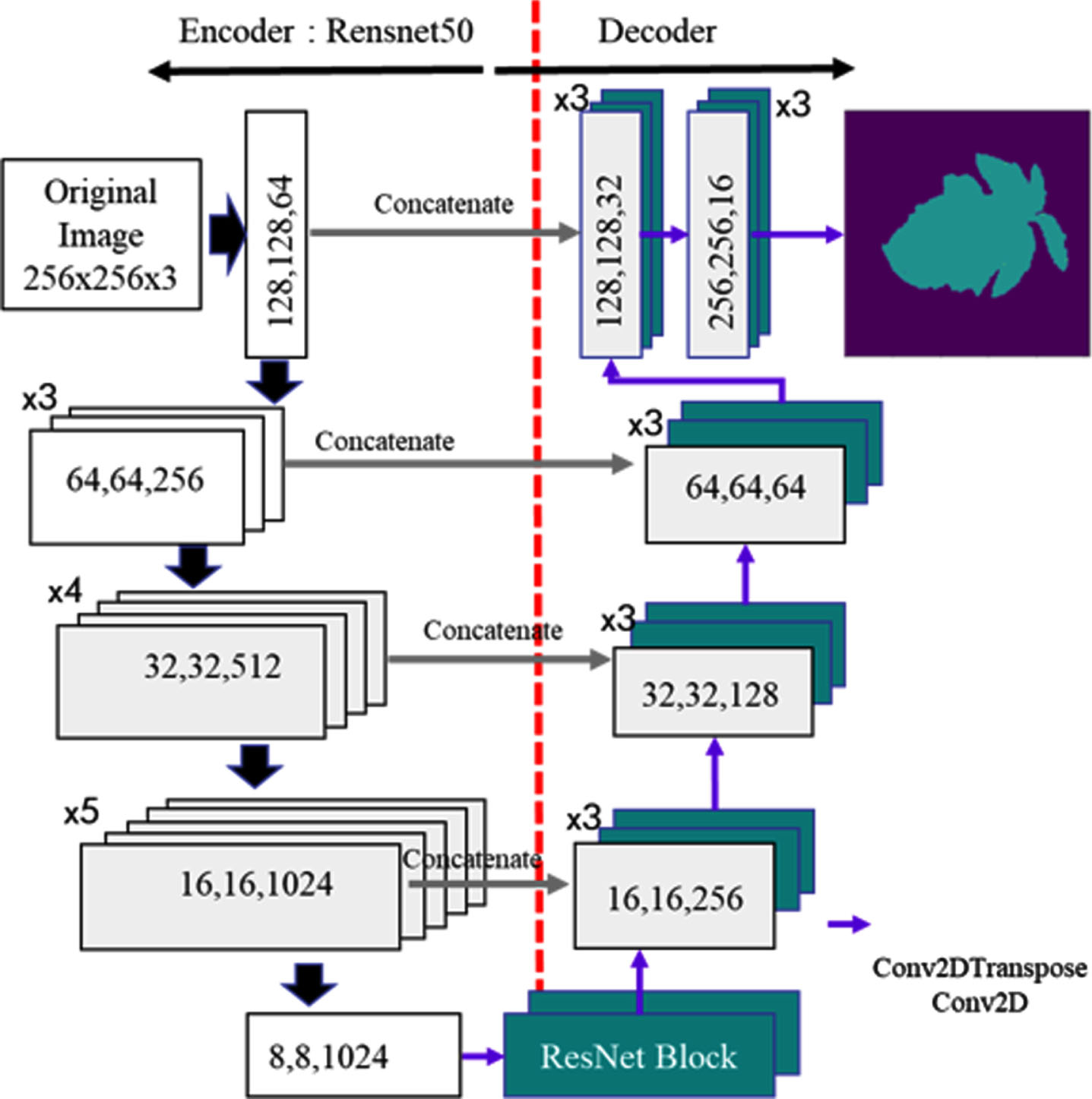
U-Net architecture for generating binary images from annotated and original images.
A series of operations were performed to match the shape of images collected in the field with those in the PlantVillage dataset as shown in Fig. 4. First, we calculated the contour of the segmented image and the bounding box for images with a contour area of 1000 or less. However, the cropping step was skipped for images with contour areas greater than 1000 because it is not necessary. Then, we calculated the orientation of each leaf and rotated it for consistency since leaf orientation varied significantly in the field data.
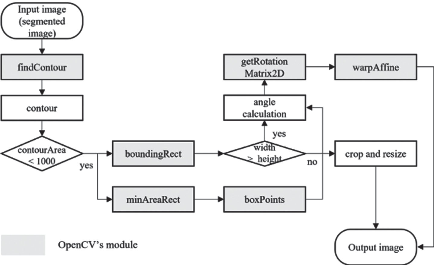
Schematic flow chart of the cropping and rotation.
Loss functions of CycleGAN
The key to CycleGAN is to change the style of the image while allowing it to remain recoverable to the original image. Put another way, it is not a simple mapping from the source domain to the target domain; a constraint is applied in consideration of returning to the original image. In this study, the CycleGAN objective function [28] comprises the GAN’s adversarial loss and cycle consistency loss, as shown in Equation (1).
Equation (2) is the objective function of GAN [29]. The generator model (G) receives the source image and target image as inputs and generates an image in the style of the target image. Assuming that a real image is 1 and fake image is 0, the discriminator trains to predict the real image as a value close to 1. In other words, it is trained to maximize D such that log(D(x)) has a probability close to 1. In contrast, the generator is updated aiming to have a probability value close to 0 for the fake image being generated. By repeating this process, the entire loss function is updated, allowing the discriminator to predict the image generated by the generator as a real image.
Equation (3) represents the cycle consistency loss and is used to check whether the image is properly restored once returned to the original domain, considering not only the mapping in one direction but also the mapping after being converted and restored again.
In the case of CycleGAN, the multiple models require a configuration for creating a multi-class domain. In general, when multiple models are configured, the model capacity grows but the memory and real-time application capacity remain limited. As shown in the CycleGAN loss in Equation (4), the method proposed in this study additionally constructs a domain classification adversarial loss [30]. Generator model G attempts to update the parameter such that the generated image can be output to the target label c.
The class discriminator uses the pretrained DensNet121 and attempts to minimize the loss of the generator generated image and target label without progressing the transfer learning. Ultimately, the CycleGAN objective function is applied as shown in Equation (5).
The generator receives a leaf disease image with a size of 256×256×3 pixels and encodes it into a feature map of 8×8×512×five convolution modules. The encoded feature map is decoded into a 256×256×128 image through a decoding process using the Conv2Dtranspose modules. The final output is a 256×256×3 image with the same size as the input. The tanh function is applied as the activation function. Each time the convolution module is passed, each image is normalized using the Instance Normalization function and LeakyReLU is applied as the activation function. In the case of the discriminator, the 256×256×3 image output by the generator is configured as a 16×16×1 feature map through the five convolution modules. This is the same as that in the generator. LeakyReLU is applied to the Instance Normalization and activation function whenever each convolution module is passed. During the training of CycleGAN, we assessed the applicability of both Batch Normalization and Instance Normalization, and discovered that Instance Normalization demonstrated superior generalization performance. We chose to apply Instance Normalization to our model as a result. The network structures of the generator and discriminator models applied in the CycleGAN are listed in Tables 2 3, respectively.
Summary of generator model
Summary of generator model
Summary of discriminator model
We predicted tomato leaf disease based on the PlantVillage dataset using different pretrained models and selected the most suitable model. ResNet50, Inception v3, and DenseNet121 were used as the pretrained models. No data augmentation was used for the learning data. The learning was conducted by categorizing the data into 10 classes and three classes. The weights of all layers were learned during the training and updated using the Adam optimizer. The initial learning rate was set to 0.001 and was set to decrease by 10% every five epochs. The learning was performed for 50 epochs. The resultant best model (DenseNet121) was used to predict diseases in the local images. There was no additional learning; the weights learned with the PlantVillage dataset were employed to classify the local image. The DenseNet121 model concatenates the feature maps of all of the layers with the input of the next layer. It improves the gradient vanishing by using a pre-activation structure such as ResNet, with the difference being that ResNet uses the sum at F(x)+x, whereas DenseNet uses concatenation. In this study, the learning was even easier even when the network was deep, as the concatenation layer had direct access to the gradient from the loss function and original input signal. Because the feature map was preserved and concatenated, DenseNet could maximize the information flow between network layers. Thus it represented an easy to learn compression model with efficient parameter usage through feature reuse.
Implementation and results
All models used in this study were executed in the Colab environment and implemented using TensorFlow’s Keras API. In this section, we present the parameters used for training and the experimental results.
Experiment setup
The U-Net model was trained for 100 epochs with a batch size of 8. Optimizer implemented Adam optimizer with an initial learning rate of 0.0001. The learning rate was dynamically reduced during training based on the validation loss using the ReduceLROnPlateau callback function. ModelCheckpoint function was used to store the precision-based weights of the best-performing model. EarlyStopping was utilized to terminate training if the validation loss did not improve for nine iterations in a row. Accuracy and sparse categorical cross-entropy were used as evaluation metrics and loss function during training.
Throughout the training of CycleGAN, 50 epochs were conducted. Due to the fact that tomato leaf diseases consist of various images the batch size was set to 1. Both the generator and discriminator’s optimizers were Adam optimizers with a learning rate of 0.0002. During the training of CycleGAN, the learning rate was maintained to prevent overfitting, which could occur when decreasing the learning rate. From the 40th epoch on, the prediction images were created on the validation dataset and the corresponding weights were saved each epoch, and the experiment weights with the sharpest images were chosen through visual inspection. The final experiments were then conducted utilizing the optimal weight parameters. 80 percent of the data in the training dataset was used for training, while 20 percent was used for validation.
The classification model utilized weights trained on the PlantVillage dataset. The model was trained for 25 epochs using the Adam optimizer with a learning rate of 0.001. After the 5th epoch, the learning rate was reduced by 10% with each subsequent epoch. The categorical cross entropy loss function was compiled, and the weights associated with the highest validation accuracy were saved. Using these final saved weights, the generated images by CycleGAN were validated.
Evaluation metrics
An F1-score [31] and confusion matrix were used to strategically evaluate the performance of the proposed approach, as follows:
In the above, TP, TN, FP, and FN represent a true positive, true negative, false positive, and false negative, respectively. The Jaccard score as expressed in Equation (7) [32] was used to evaluate the performance of the segmented image and to determine the similarity between the two sets. In addition to the quantitative evaluation, the Grad-CAM [33] algorithm was used in the classification model to qualitatively assess whether the disease sites were correctly diagnosed.
To assess the quality of the artificial images produced by CycleGAN, we utilized measures of image quality, including the Peak Signal-to-Noise Ratio (PSNR) and the Inception Score (IS). The Inception score is a metric developed by Google to evaluate the quality of images generated by GANs [34]. The Inception score was calculated based on the probability vector generated by amplifying the images with Google’s Inception V3 model. Here KL divergence was used to measure how similar or different two probability distributions are. The higher the inception score, the better the quality, and it can be calculated using Equation (8).
Performance of the segmentation model
Figure 5 presents the segmentation performance visually, and the effect of removing the background from the original images was confirmed.
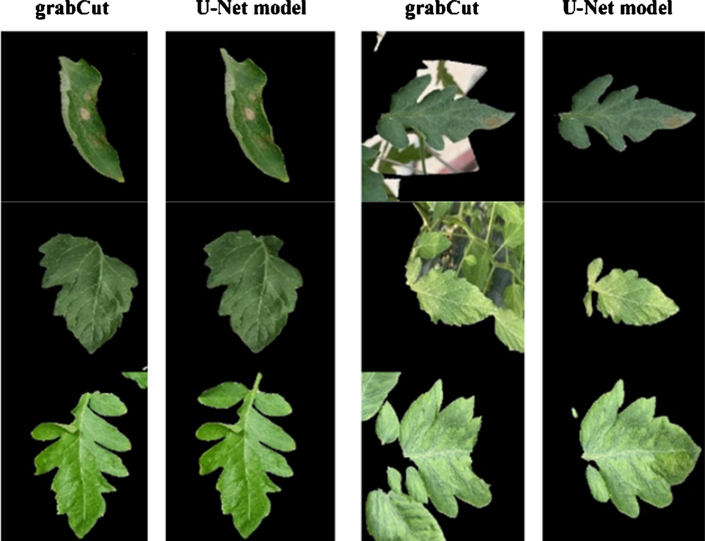
Segmented images of grabCut and U-Net segmentation model. The background was not completely removed from the grabCut images.
Even with a complex background, the image of the area of interest is properly segmented. The Jaccard score (a quantitative evaluation index) averages 0.98, confirming that the training is well-managed. Furthermore, using OpenCV’s grabCut module, it can be confirmed that the model properly segments images for with difficult to remove backgrounds.
The effects of data preprocessing during the CycleGAN training were investigated. Table 4 represents images generated by CycleGAN before and after preprocessing. The image quality was predicted to be significantly lower without any preprocessing to the extent that it could be visually discerned. Hence, we had to perform the preprocessing proposed in this study to exhibit characteristics as much as the PlantVillage images.
Generated images before and after applying image preprocessing
Generated images before and after applying image preprocessing
Figure 6 demonstrates the CycleGAN training results for the preprocessed images. The U-Net based segmentation model showed excellent performance without loss of generality such as disease regions. Additionally, the PSNR values and Inception Scores between the original and synthesized images were evaluated to understand CycleGAN performance as shown in Table 5. These PSNR values were similar to the results of the C-GAN proposed by ABBAS [19]. It demonstrated that the quality of the images generated by CycleGAN is very close to that of the real images.
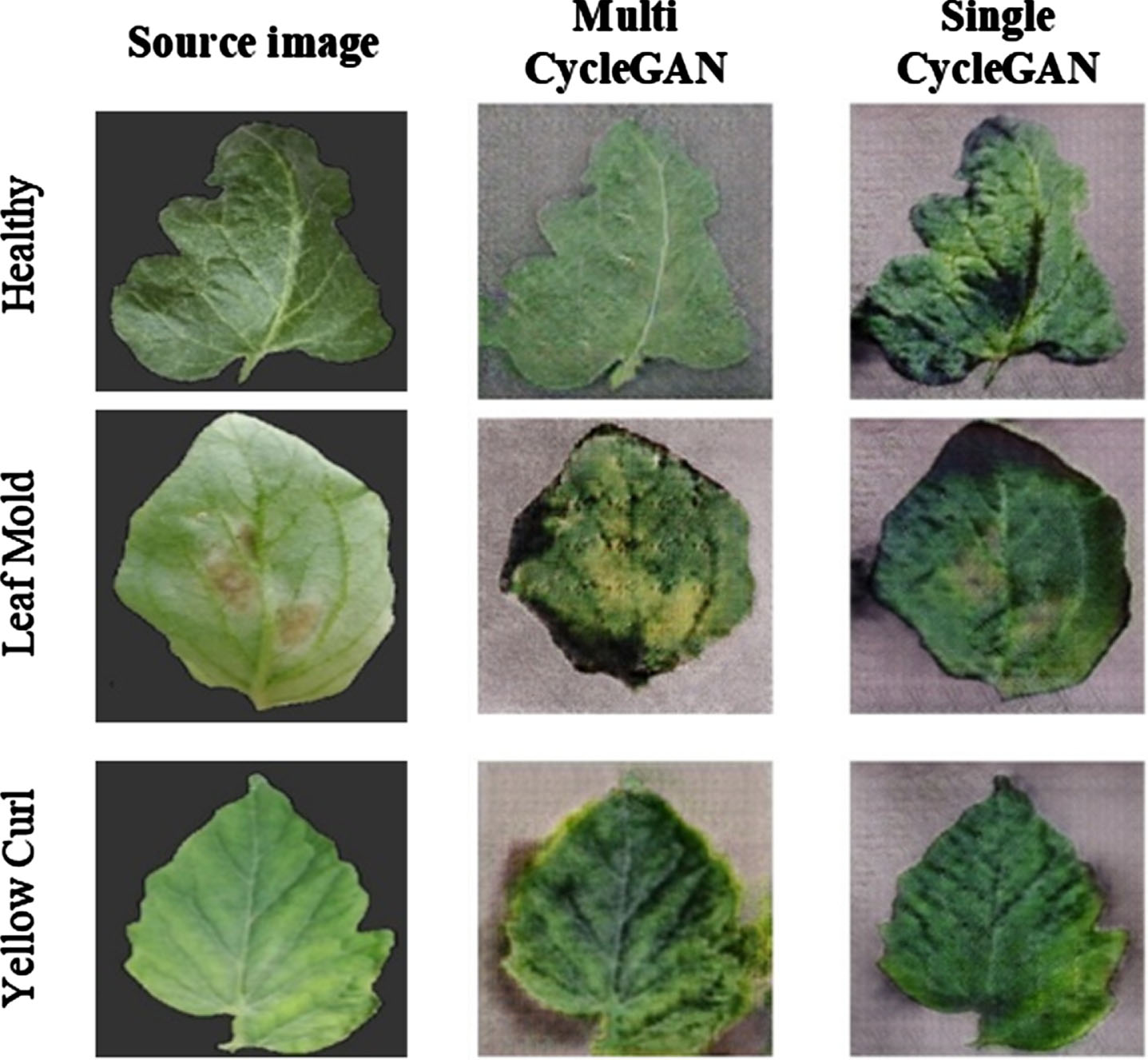
Examples of generated images by CycleGAN. Here, the image preprocessing was applied successfully to maintain important features of the original images, such as disease regions, while altering other stylistic elements.
Prediction performance of generated tomato images by CycleGAN
Overall, the local image’s style has been adapted to match that of the PlantVillage dataset. Furthermore, in the case of a disease image, the loss of the disease area is insignificant and both the normal and diseased areas are well expressed. Additionally, the generated images had a high level of visual quality, indicating the effectiveness of the image processing used.
The performances of the images from PlantVillage datasets from three class were evaluated. As mentioned above, the pretrained models ResNet50, InceptionV3, and DenseNet121 were used to classify the images. ResNet50, Inception V3, and DenseNet121 are state-of-the-art models in image classification. All three models demonstrated prediction accuracies of over 95% in classifying tomato leaf diseases [35].
As a result of the image classification, all models performed exceptionally well in terms of the quantitative evaluation index, as shown in Table 6. The disease areas were visualized as shown in Fig. 7, to determine whether the Grad-CAM algorithm correctly judged the disease area. As can be seen, DenseNet121 correctly identified the disease and performed the best on the same image. Finally, the DenseNet121 model was used to classify three classes of images generated by CycleGAN.
F1-score results for models trained from PlantVillage dataset
F1-score results for models trained from PlantVillage dataset
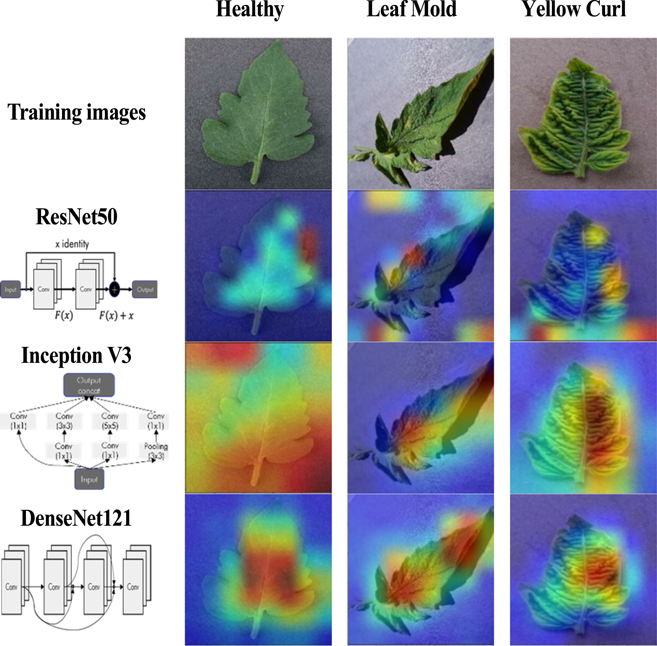
The gradCAM results of the PlantVillage dataset. It shows that each transfer learning model accurately identifies disease areas, with DenseNet121 being the most precise in identifying the disease regions.
The classification results were shown in Table 7. Without the CycleGAN based domain adaptation, the F1-score was 50%; with the proposed method, it reached 96.3%. The proposed method achieved a performance of 95.6% for images generated with domain classification adversarial loss models.
Classification performance based on DenseNet121
The Multi CycleGAN and Single CycleGAN differ according to whether the class was trained concurrently or sequentially. When we evaluated the classification performance on images generated by two different CycleGAN models, the accuracy, F1-score, precision, and recall scores all showed outstanding performances. Figure 8 displays the Confusion Matrices to evaluate the classification performance of tomato disease images generated by CycleGAN. As a result, the classification performance of the two CycleGAN models exceeded that of the original images. However, for a single CycleGAN model, while it could generate images with multiple labels, its classification accuracy was lower than that of the Multi CycleGAN due to the lack of dataset. It is expected that even the single model is able to demonstrate high performance when the amount of data collected in the field is sufficient.
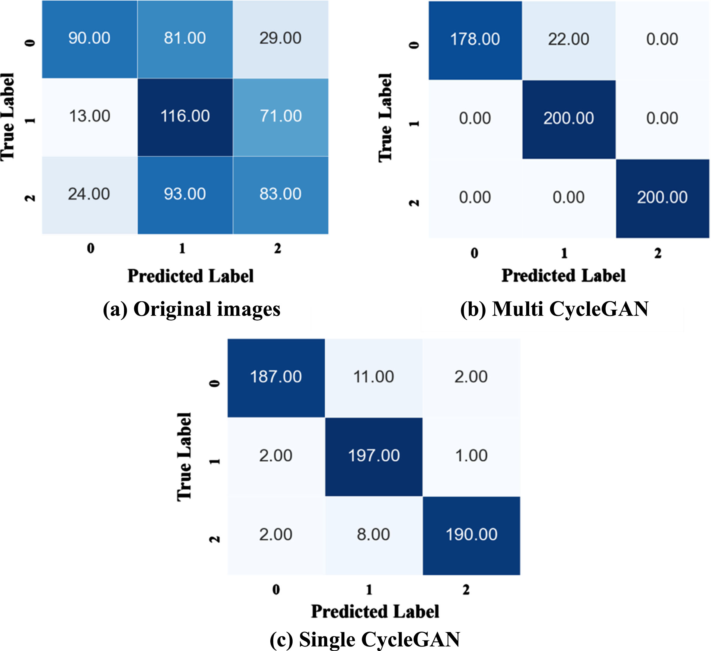
Confusion matrix of classification results: (a) classification re-sults of original images, (b) classification results of generated images by multi CycleGAN based on basic loss, (c) classification results of generated images by singleCycleGAN based on domain classification adversarial loss. 0: Leaf mold, 1: Yellow leaf curl virus, 2: Healthy.
In this study, we discussed a domain adaptation methodology with a PlantVillage dataset related to tomato leaf disease and datasets collected in the field. CycleGAN is used in a variety of fields; in this study, we used it to introduce a cyclic consistency loss function for transferring the color texture while maintaining the shape of the object, even when the image was unpaired.
The quality of input images is crucial for improving the generalization performance of deep learning models. In the training of the CycleGAN model used in this research, preprocessing of input data was also a critical factor. We emphasized the importance of image preprocessing in this paper. Although there were cases where the generalization performance was compromised during the training of images processed with the proposed preprocessing methods, this issue was resolved by appropriately combining instance normalization and batch normalization in the configuration of the training layers. Furthermore, the choice of loss functions for the discriminator and generator had an impact on the generalization performance, with differences observed between binary cross-entropy and mean absolute error functions. Other factors such as activation functions, epoch count, and learning rate were also considered when determining the final parameters, and it was observed that these parameters had a significant influence depending on the training data.
Ultimately, the proposed CycleGAN model aimed to transform images of three different diseases with a single training process. This approach was proposed with a focus on practical applicability in the field. For real-time disease detection during measurement, a lightweight model was necessary, and the proposed Single CycleGAN was considered capable of achieving this. Moreover, for diseases on leaves in greenhouses, where color differences clearly indicate disease presence, it is possible to achieve early detection using machine learning models rather than deep learning models. If a state-of-the-art model like CycleGAN is applied to disease classification based on these early-detected disease images, it is expected to lead to the development of better field-applicable applications.