ComMatch: A semi-supervised learning classification algorithm based on model calibration

Abstract

Semi-supervised learning (SSL) aims to reduce reliance on labeled data. Achieving high performance often requires more complex algorithms, therefore, generic SSL algorithms are less effective when it comes to image classification tasks. In this study, we propose ComMatch, a simpler and more effective algorithm that combines negative learning, dynamic thresholding, and predictive stability discriminations into the consistency regularization approach. The introduction of negative learning is to help facilitate training by selecting negative pseudo-labels during stages when the network has low confidence. And ComMatch filters positive and negative pseudo-labels more accurately as training progresses by dynamic thresholds. Since high confidence does not always mean high accuracy due to network calibration issues, we also introduce network predictive stability, which filters out samples by comparing the standard deviation of the network output with a set threshold, thus largely reducing the influence of noise in the training process. ComMatch significantly outperforms existing algorithms over several datasets, especially when there is less labeled data available. For example, ComMatch achieves 1.82% and 3.6% error rate reduction over FlexMatch and FixMatch on CIFAR-10 with 40 labels respectively. And with 4000 labeled samples, ComMatch achieves 0.54% and 2.65% lower error rates than FixMatch and MixMatch, respectively.

Keywords

Semi-supervised learning negative learning dynamic threshold predictive stability

1 Introduction

The rise of deep learning has led to significant performance improvements in computer vision tasks, but achieving these gains typically requires large labeled datasets. However, annotation for tasks such as classification, detection, and segmentation can be costly and may require expert input. In comparison, unlabeled data is easier and less expensive to obtain [10, 15].

Semi-supervised learning (SSL) [5] is a powerful approach that combines supervised and unsupervised learning to effectively address the problem of insufficient labeled data. However, one of the primary challenges with SSL is how to learn from large amounts of unlabeled data. Many approaches have been proposed in the research of SSL, including consistency-regularization [21, 29] and pseudo-labeling [22, 27], among others. The method based on consistency-regularization encourages the model to produce consistent output distributions even when subjected to varying degrees of input perturbations, thereby enhancing the model’s robustness. The pseudo-labeling-based approach trains the model on labeled data and then selects unlabeled samples with high confidence as new training targets. Compared to the consistency-regularization-based approach, the pseudo-labeling-based approach does not rely on data augmentation and can have implementation value in various domains. It’s worth noting that generating pseudo-labels typically requires an argmax operation to classify data into one of the categories. However, when the number of labeled data is limited, the classification effect of the trained classification network may not be convincing, resulting in overconfidence and false pseudo-labeling.

In this paper, we propose ComMatch, a new SSL algorithm that combines consistency regularization, pseudo-labeling, negative learning, and predictive stability. We use weak augmentation on unlabeled data to select pseudo-labels, including both positive and negative ones, and leverage RandAugmet [9] for strong augmentation. ComMatch introduces a comprehensive loss that includes both supervised and unsupervised loss. The unsupervised loss is obtained utilizing pseudo-labeling. Based on the idea of negative learning, we divide the unsupervised loss into two parts and finally combine the supervised loss for training to get the final classification network. We show that ComMatch obtains great performance on the SSL benchmarks. For instance, on the CIFAR-10 dataset, ComMatch achieves 91.75%, 95.26%, and 96.08% accuracy when the label amount is 40, 250, and 1000 respectively. According to the results, there is a certain improvement over the previous SSL algorithms.

The main contributions are as follows:

Incorporating the idea of negative learning, our method improves the accuracy of positive pseudo-labels while reducing the confidence of mislabeled data by including categories below a low threshold as negative labels in the label prediction process.

Designing a dynamic threshold-based pseudo-label selection mechanism, which adjusts the threshold value dynamically with each iteration of the training process. As the number of training rounds increases, the threshold is scaled accordingly, helping to improve the convergence speed of the model.

Introducing a new metric, network predictive stability, which indirectly reflects the matching degree between the network’s confidence and accuracy. During the selection process of positive and negative pseudo-labels, the metric can reduce the impact of erroneous predictions caused by poor model calibration, thus improving the robustness of the method and the reliability of classification of unlabeled data.

2 Related work

Semi-supervised learning is a broad field in which many methods have matured to improve the performance of networks by learning useful information from unlabeled data. In this part, we focus on the components used in ComMatch, such as consistency regularization, entropy minimization and pseudo-labeling, etc. Some other SSL methods are not discussed here (such as “transductive” models, graph-based methods, generative modeling, etc.).

2.1 Consistency regularization

As one of the most widely used approaches in SSL, consistency regularization is inspired by regularization techniques for data augmentation in supervised learning. This method artificially expands the dataset without changing the labels of the images. It works by elastically deforming or adding noise to the input images. This ensures that the distribution of the classifier output remains unchanged when the input is perturbed to varying degrees. Consistency regularization was first proposed in [1], and common approaches to random perturbation include data augmentation and random regularization, etc. Many excellent semi-supervised algorithms, such as CoMatch [23], now incorporate consistency regularization. Generally, consistency regularization can be achieved by the following loss term [21, 29]:

$\begin{matrix} ∥ P_{model} (y | {Augment}_{1} (x); θ) \\ {- P_{model} (y | {Augment}_{2} (x); θ) ∥}_{2}^{2} \end{matrix}$ (1) where x represents the input, y represents the output, and θ represents other parameters in network training. Augment (x) refers to a random augmentation. As such,Augment₁ (x) and Augment₂ (x) are randomly different.

2.2 Entropy minimization

The clustering assumption in SSL is also referred to as the low-density separation assumption, which states that the decision boundary of the classifier should be located in a low-density region. By using this method, the classifier can separate unlabeled data and make high-confidence predictions. The model makes low-entropy predictions on the unlabeled data by using the one-hot labels constructed from the high-confidence output categories to calculate cross-entropy loss with their output distribution, thereby achieving entropy minimization. In [4], the “sharpening” function is also used to reduce the entropy of the predicted labels. In most methods, the weak augmentation version is used as the target for the strong augmentation version in cross-entropy loss. However, the pseudo-labels predicted by the classifier trained only on limited labeled data often suffer from confirmation bias, which can lead to errors in learning.

2.3 Pseudo-labeling

The process of generating pseudo-labels [22, 27] involves the classifier creating artificial labels for unlabeled data by making predictions. In [22], it is suggested that pseudo-labels are the categories with the highest output probability for the unlabeled samples, as determined by the trained network. Iscen, Ahmet, et al. [16] propose a way to provide pseudo-labels for unlabeled samples through a neighborhood graph. The use of pseudo-labels is the minimum requirement in this case. FlexMatch [35] determines the appropriate confidence threshold for generating pseudo-labels for training based on the network’s prediction difficulty for different categories. By comparing the model’s prediction with the threshold, either “positive” learning or “negative” learning can be executed [19]. However, the accuracy of pseudo-labels heavily depends on the quality of the classifier’s predictions, and accumulating misclassifications during the prediction process can result in confirmation bias.

2.4 Model Calibration

Calibration refers to the overall uncertainty of a network’s predictions. In [27], a line chart of prediction uncertainty-prediction calibration error demonstrates that high-confidence network predictions often result in correct pseudo-labels. In a decision-making classification network, it’s important to not only ensure higher accuracy but also to indicate when the prediction is incorrect. This means the network should provide a calibrated confidence measure [13] in addition to its prediction. In semi-supervised learning, confirmation bias often occurs due to the model’s erroneous predictions, which are mainly caused by the network’s overconfidence in the self-training process. Therefore, model calibration is closely related to confirmation bias. To better train the network, the measure of model calibration should be added to the training process to improve the network’s generalization ability.

3 ComMatch

In this section, we will introduce the details of the semi-supervised learning method ComMatch. ComMatch combines consistency regularization and pseudo-labeling to update the classifier through the model calibration, dynamic threshold, and negative learning during the training process, as shown in Fig. 1. In addition, the method employs weak and strong augment strategies for images respectively, Specifically, it uses [9] as the strong augmentation method and randomly selects from a fixed set of geometric and intensity transformations [8] to increase the randomness and diversity of the images, helping the network to learn more details in the images. For multi-class classification problems, let D_l ={ (x_b, y_b) ; b ∈ 1, …, B_l } be a batch of labeled data and D_u ={ (u_b) ; b ∈ 1, …, B_u } be a batch of unlabeled data, where x_b and u_b represent the labeled and unlabeled training samples, y_b represents the hard label of the bth sample, B_l and B_u represent the number of labeled data and unlabeled data, respectively. Let p_model (y|x) represent the class distribution predicted by the classification network. Aug_w (·) and Aug_s (·) represent weak and strong augmentation, respectively. The schematic diagram of ComMatch is shown in Fig. 1, and the specific algorithm is shown in Algorithm 1.

Fig. 1

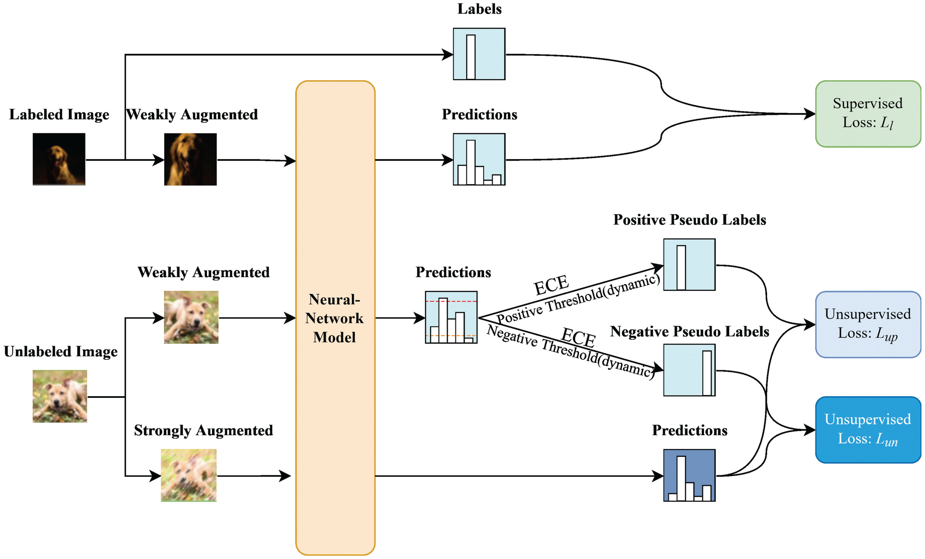
Diagram of ComMatch. The labeled data are weakly augmented and fed into the classification network for prediction, and then cross-entropy loss is performed with the corresponding labels; Meanwhile, the unlabeled data are fed into the network for prediction after weak and strong augmentation respectively, where the weakly augmented version is filtered to obtain positive and negative pseudo-labels, and they generate unsupervised losses with the strongly augmented version of the prediction.

During the training iteration, ComMatch updates the network based on three types of losses: (1) supervised classification loss L_l between the prediction and label of labeled data, (2) unsupervised classification loss L_Pu between positive pseudo-labels and the predicted distribution of unlabeled data, and (3) negative cross-entropy loss L_Nu between negative pseudo-labels and the predicted distribution of unlabeled data. Specifically, the supervised loss of labeled data is represented by the cross-entropy loss between the label and the model’s prediction: $L_{l} = \frac{1}{B_{l}} \sum_{b = 1}^{B_{l}} H (y_{b}, p_{model} (y | {\hat{x}}_{b}))$ (2) where y_b represents the hard label (one-hot) of the input sample x_b, ${\hat{x}}_{b}$ denotes the weakly augmented form of the input sample x_b, p_model (y|x) denotes the class distribution predicted by the classification network, and H (a, b) denotes the cross-entropy loss between the distributions a and b.

3.1 Confidence-based pseudo-label selection

The selection of pseudo-labels in network training includes positive and negative pseudo-labels. The selection of positive pseudo-labels conforms to positive learning, where the one-hot label is obtained through the prediction of the maximum category during network prediction. Before training the network, we set a high threshold to filter out low-confidence pseudo-labels in the early stage of training. As the training progresses and the model accuracy improves, high-confidence predictions are selected as positive pseudo-labels, represented as: $1 [p_{model} (y | {\hat{u}}_{b}) ⩾ t_{p}]$ (3) where ${\hat{u}}_{b}$ is the weak augmentation form of unlabeled input u_b, and t_p is a predetermined threshold with a large value.

Negative learning can comprehensively learn the features and distribution of samples, providing additional information gain. More importantly, in the early stages of training, the model is more confident in determining that a sample does not belong to a category rather than belonging to a category. ComMatch adopts the idea of negative learning, pushing the probability of negative pseudo-labels towards 0. As a result, the predicted probabilities of other categories naturally increase, indirectly promoting positive learning effects. This is advantageous in reducing the impact of noise and inaccurate labels on training. To implement this indirect learning approach, we can select some “high-confidence labels that do not belong to the class” as negative pseudo-labels. Before training the network, we set a low threshold to filter out classes with predicted confidence lower than the pre-set low threshold during training. This is represented as: $1 [p_{model} (y | {\hat{u}}_{b}) ⩽ t_{n}]$ (4) where t_n is a pre-set threshold with a small value.

3.2 Dynamic adjustment of thresholds

In network training, previous research has employed a fixed high threshold to select positive pseudo-labels with a certain level of confidence, but overlooked the effect of low confidence categories on training, leading to potential wastage of training samples. This is especially true during the early stages of training when the network may not have sufficient training on input samples, resulting in the neglect of a large portion of the samples and slow convergence. Thus, we propose a strategy that dynamically adjusts the threshold size based on the training progress. Especially, the model’s representation of the distribution and characteristics of unlabeled data is not accurate enough in the early stages of training. Therefore, more samples need to be added for training. This dynamic threshold setting mechanism will learn more accurate feature boundaries as the training progresses, thereby continuously raising the screening criterion to increase the propagation of accuracy in later training, helping us better utilize unlabeled data to improve performance. In particular, the threshold can be scaled based on the changes in network parameters during training, as shown below: $t_{p} = α_{epoch}^{p} + t_{p 0}$ (5) $t_{n} = α_{epoch}^{n} \cdot t_{n 0}$ (6) in the above formulas, t_p0 and t_n0 represent the initial thresholds for positive and negative learning, respectively. $α_{epoch}^{p}$ is an additive parameter that changes dynamically with iteration cycles, while $α_{epoch}^{n}$ is a dynamic scaling factor that changes with iteration cycles. As the confidence trends of positive and negative samples vary differently during training, we employ distinct threshold adjustment strategies to better fit the data. Compared to a fixed threshold, a dynamic threshold can fully leverage training data in the early stages of training by selecting higher confidence categories as positive pseudo-labels, ultimately boosting network prediction accuracy and accelerating convergence.

3.3 Stability discrimination of network predictions

The process of network calibration aims to ensure that the predicted probability of the model aligns with the true probability. Although the model’s average confidence in the test set tends to be high after training, its actual accuracy often falls below this level, revealing the model’s tendency to overestimate its performance. To address this issue, Guo, Chuan, et al. [13] proposes the use of expected calibration error (ECE), which measures the expected difference between confidence and accuracy, as a metric for evaluating network calibration. By minimizing ECE during training, the model’s predictions can become more accurate and the accuracy of pseudo-labels can be improved.

Using a threshold to screen pseudo-labels can significantly reduce the error rate by including high-confidence positive and low-confidence negative pseudo-labels in training. However, if the model’s calibration is not good, prediction errors can accumulate, leading to confirmation bias. A perfectly calibrated model should achieve the same accuracy and confidence as the model itself, as shown by the following equation: $P (\hat{Y} = Y | \hat{P} = p) = p, \forall p \in [0, 1]$ (7) in the equation, $\hat{Y}$ represents the model’s predicted output, Y represents the true label of input x, and $\hat{P}$ represents the model’s confidence. What factors contribute to the deviation between the overall prediction uncertainty and individual prediction uncertainty of the network?

In model training process, we introduce the Dropout [24] method to increase randomness and reduce co-adaptation between neurons, making the model’s multiple results with randomness for the same input. Therefore, the differences among random results can be considered as a measure of prediction instability, denoted as “u". Specifically, prediction instability is the standard deviation of the probability output calculated based on the number of loops, where the probability output is obtained by applying Softmax to the outputs of 10 loops on a batch of samples. The mathematical expression is as follows: $u (p_{model} (y | {\hat{u}}_{b})) = \sqrt{\frac{1}{N_{c}} \sum_{i = 1}^{N_{c}} {(p_{model}^{i} (y | {\hat{u}}_{b}) - \bar{X})}^{2}}$ (8) where N_c represents the number of loops, and $p_{model}^{i} (y | {\hat{u}}_{b})$ represents the probability output of the class corresponding to $\bar{X}$ in the i-th loop. $\bar{X}$ equals $1 / - N_{c} \cdot \sum_{i = 1}^{N_{c}} p_{model}^{i} (y | {\hat{u}}_{b})$ , representing the maximum mean value of predicted outputs over N_c loops. We verify on different datasets that the stability of network predictions does indeed affect the change in ECE, as shown in Fig. 5. In the range of 0 to 0.05 (the larger value between s_p and s_n) for prediction instability, higher instability leads to larger ECE values. Conversely, lower instability leads to smaller ECE values. Therefore, we use the instability metric as one of the criteria for selecting pseudo-labels to improve the reliability of model predictions. The subsequent process of pseudo-label selection can be represented as follows: $g_{p} = 1 [p_{model} (y | {\hat{u}}_{b}) ⩾ t_{p}] \cdot 1 [u (p_{model} (y | {\hat{u}}_{b})) ⩽ s_{p}]$ (9) $g_{n} = 1 [p_{model} (y | {\hat{u}}_{b}) ⩽ t_{n}] \cdot 1 [u (p_{model} (y | {\hat{u}}_{b})) ⩽ s_{n}]$ (10) where u (·) represents the measure of prediction instability, and it is referred to as the stability discrimination. t_p and t_n denote the dynamically adjusted thresholds for positive and negative learning, while s_p and s_n refer to the prediction stability thresholds for positive and negative learning, respectively. g_p and g_n denote whether the positive and negative pseudo-labels are selected for training, with values of 0 and 1 indicating non-selection and selection, respectively. It is worth noting that the $p_{model} (y | {\hat{u}}_{b})$ compared with t_p and t_n is not the same as the $p_{model} (y | {\hat{u}}_{b})$ used in calculating stability measures. The former is a specific value calculated separately after determining the model stability in the current round of training, while the latter refers to the notation of model predictions in calculating model stability.

The unsupervised loss includes fitting the strong augmented samples to positive pseudo-labels and separating from negative pseudo-labels (not fitting), thus expanding the information gain of the samples themselves. The corresponding positive pseudo-label loss $L_{Pu}^{b}$ and negative pseudo-label loss $L_{Nu}^{b}$ are as follows: $L_{Pu}^{b} = - \sum_{c = 1}^{C} g_{p} \cdot q_{Pb} \log (p_{model} (y | {\tilde{u}}_{b}))$ (11) $L_{Nu}^{b} = - \sum_{c = 1}^{C} g_{n} \cdot (1 - q_{Nb}) \log (1 - p_{model} (y | {\tilde{u}}_{b}))$ (12) here, g_p and g_n are binary variables with values of 0 and 1. $q_{Pb} = \underset{c}{argmax} p_{model} (y | {\hat{u}}_{b})$ represents the selected positive pseudo-label (one-hot), while $q_{Nb} = \underset{c}{argmin} p_{model} (y | {\hat{u}}_{b})$ denotes the selected negative pseudo-label. After traversing all data, the losses in equations and are accumulated to yield the unsupervised losses L_Pu for positive learning and L_Nu for negative learning. The weighted sum of the supervised and unsupervised losses produces the total loss: $L = L_{l} + λ L_{Pu} + μ L_{Nu}$ (13) where λ and μ are the weight coefficients of the unsupervised loss relative to the supervised loss.

3.4 Augmentation Strategy for ComMatch

ComMatch employs two types of augmentation strategies to alleviate the problem of scarce labeled training samples: weak augmentation and strong augmentation. Specifically, weak augmentation utilizes random horizontal flipping and shifting. On the other hand, strong augmentation consists of two augmentation techniques, namely RandAugment [9] and CTAugment [4]. RandAugment randomly selects multiple augmentation transformations from a predefined set of geometric, color, and other transformations. For each transformation, a random strength parameter is selected to control the intensity of the transformation. CTAugment is an adaptive augmentation method that selects and applies specific perturbations based on the predicted class of the image.

Algorithm 1: ComMatch
Input: Batch of labeled examples and their one-hot labels D_l ={ (x_b, y_b) ; b ∈ 1, …, B_l }, batch of unlabeled examples D_u ={ (u_b) ; b ∈ 1, …, B_u }, unsupervised loss weight λ,μ, high threshold t_p, low threshold t_n.
Output: Updated model.
1: forb = 1 to B_ldo
2: ${\hat{x}}_{b} = {Aug}_{w} (x_{b})$
3: end for
4: $L_{l} = \frac{1}{B_{l}} \sum_{b = 1}^{B_{l}} H (y_{b}, p_{model} (y \| {\hat{x}}_{b}))$
5: forb = 1 to B_udo
6: ${\hat{u}}_{b} = {Aug}_{w} (u_{b})$
7: ${\tilde{u}}_{b} = {Aug}_{s} (u_{b})$
8: $q_{Pb} = \underset{c}{argmax} p_{model} (y \| {\hat{u}}_{b})$
9: $q_{Nb} = \underset{c}{argmin} p_{model} (y \| {\hat{u}}_{b})$
10: $g_{p} = 1 [p_{mod el} (y \| {\hat{u}}_{b}) ⩾ t_{p}] \cdot 1 [u (p_{mod el} (y \| {\hat{u}}_{b})) ⩽ s_{p}]$
11: $g_{n} = 1 [p_{mod el} (y \| {\hat{u}}_{b}) ⩽ t_{n}] \cdot 1 [u (p_{mod el} (y \| {\hat{u}}_{b})) ⩽ s_{n}]$
12: $N_{p} = \sum_{c = 1}^{C} g_{p}$
13: $N_{n} = \sum_{c = 1}^{C} g_{n}$
14: $L_{Pu}^{b} = - \sum_{c = 1}^{C} g_{p} \cdot q_{Pb} \log (p_{model} (y \| {\tilde{u}}_{b}))$
15: $L_{Nu}^{b} = - \sum_{c = 1}^{C} g_{n} \cdot (1 - q_{Nb}) \log (1 - p_{model} (y \| {\tilde{u}}_{b}))$
16: end for
17: $L_{Pu} = \frac{1}{N_{p}} \sum_{b = 1}^{B_{u}} L_{Pu}^{b}$
18: $L_{Nu} = \frac{1}{N_{u}} \sum_{b = 1}^{B_{u}} L_{Nu}^{b}$
19: update all parameters according to:
L = L_l + λL_Pu + μL_Nu

4 Experiments

In our experiments, we conduct experiments to evaluate the effectiveness of ComMatch on several standard semi-supervised benchmarks. Specifically, we compare the accuracy of ComMatch on different datasets with varying amounts of labeled data to assess its performance under different scenarios. Additionally, we conduct ablation experiments to determine the contribution of each component of ComMatch to the overall performance. By conducting these experiments, we aim to gain insights into the strengths and weaknesses of ComMatch and identify areas for potential improvement.

4.1 Datasets

We conduct experiments on three different standard datasets, CIFAR-10, CIFAR-100 [20], and SVHN [24]. CIFAR-10 and CIFAR-100 contain 60,000 32*32 images, with 50,000 images for training and 10,000 for testing. CIFAR-10 has 10 categories, while CIFAR-100 has 100 categories. The SVHN dataset consists of cropped 32*32 images of house numbers from Google Street View, which has 26,032 images for testing and 73,257 for training. Different datasets are validated using varying amounts of labeled data.

4.2 Implementation details

For CIFAR-10, CIFAR-100 and SVHN, we use almost identical hyperparameters, with slight differences in the backbone networks. We use WideResNet-28-2 [34] as the backbone network during training for CIFAR-10 and SVHN, and WideResNet-28-8 for CIFAR-100. We set the initial confidence thresholds to t_p0 = 0.9 and t_n0 = 0.3, and as the training progressed, we increase t_p by 0.01 every three epochs, up to 0.95, and decrease t_n by a factor of 10 every three epochs, down to 0.0003. We evaluate the model using an exponential moving average (EMA) with a decay rate of 0.999 for the parameters. Other hyperparameters including lr = 0.03, batch_size = 64, batch size for unlabeled data = 5*64, stability threshold of s_p = 0.05, and s_n = 0.005 are listed in Table 1.

Table 1
List of ComMatch hyperparameters on the CIFAR-10, CIFAR-100 and SVHN datasets

CIFAR-10 CIFAR-100 SVHN

t _p0 0.9

t _n0 0.3

$α_{epoch}^{p}$ 0.001 · (epoch - 1)

$α_{epoch}^{n}$ $10^{- (\frac{epoch}{3} + 1)}$

s _p 0.05

s _n 0.005

λ 1

μ 2

N _c 10

lr 0.03

Batch _s ize 64

Weight _d ecay 0.0005 0.001 0.0005

	CIFAR-10	CIFAR-100	SVHN
t _p0		0.9
t _n0		0.3
$α_{epoch}^{p}$		0.001 · (epoch - 1)
$α_{epoch}^{n}$		$10^{- (\frac{epoch}{3} + 1)}$
s _p		0.05
s _n		0.005
λ		1
μ		2
N _c		10
lr		0.03
Batch _s ize		64
Weight _d ecay	0.0005	0.001	0.0005

During the early stages of training, the accuracy of positive pseudo-labels based on threshold selection in positive learning can be suboptimal due to limited data, few iterations, and noisy datasets. However, we can mitigate this issue by performing negative learning to filter out negative pseudo-labels. In negative learning, we set a fixed and low threshold to filter out low confidence error categories. Furthermore, the learning and generalization capabilities of the neural network can fit the labeled data at the beginning of training, which means that there is no situation where the correct label becomes the lowest predicted category and falls below the low threshold we set. Therefore, negative learning is much more accurate compared to positive learning.

To prioritize the accuracy of negative learning, we adjust the values of two parameters in unsupervised loss, λ and μ, and set λ to be smaller than μ so that negative learning dominates. This approach ensures that we can achieve high accuracy even in areas where prediction accuracy is critical, such as clinical and autonomous driving applications. Ultimately, by prioritizing negative learning over positive learning, we can ensure that our model achieves high accuracy while minimizing the impact of noisy datasets and other challenges in the training process.

4.3 Result

We conduct comparative experiments on the three datasets mentioned in Section 4.1, using varying amounts of labeled data ranging from 0.5% to 20%. In the experimental setup, ComMatch is benchmarked against previous SSL methods, including Mean Teacher [31], MixMatch [3], UDA [33], ReMixMatch [4], FixMatch [30], FlexMatch [35] and UPS [27].

CIFAR-10 and CIFAR-100

For CIFAR-10 and CIFAR-100, we respectively use 40, 250, and 4,000 labeled images to evaluate the accuracy of each method for the former, and 400, 2,500, and 10,000 labeled images for the latter. shows our experimental results, indicating that for CIFAR-10 with 250 and 4,000 labeled images, we achieve better results than a series of methods such as MixMatch and FixMatch. Figure 2(a) shows the loss change of ComMatch during training, and Fig. 2(b) demonstrates the comparison between ComMatch and FixMatch. Figure 2(b) only shows the results of the last 250 epochs because the model converged at around 800 epochs, and the subsequent 200+ epochs clearly demonstrate the comparative performance in accuracy between ComMatch and FixMatch.

Fig. 2

Convergence analysis of ComMatch and comparison with FixMatch on CIFAR-10-4000. (a) shows the variation of supervised and unsupervised losses during ComMatch training; (b) presents a detailed comparison of the accuracy of ComMatch and FixMatch in the last 250 epochs after ComMatch convergence.

SVHN

As a more complex dataset than MNIST, SVHN contains a larger amount of data with more diverse and complex images featuring different fonts, orientations, and backgrounds, making it more challenging to learn from. However, as a balanced dataset with ten categories, it is beneficial for models to learn the inherent patterns in the data. Table 2 shows the specific results obtained for this dataset.

Table 2

The top-1 error rates of different algorithms on three datasets, CIFAR-10, CIFAR-100, and SVHN, where each dataset contains three different amounts of labeled data

Method	CIFAR-10			CIFAR-100			SVHN
	40labels	250labels	4000labels	400labels	2500labels	10000labels	40labels	250labels	1000labels
Mean Teacher	–	32.32 ± 2.30	9 . 19 ± 0 .19	–	53 . 91 ± 0 . 57	35 . 90 ± 0 . 24	–	3 . 57 ± 0.11	3 . 42 ± 0.07
MixMatch	47.54 ± 11.50	11.05 ± 0.86	6.42 ± 0.10	67.61 ± 1.32	39.94 ± 0.37	29.02 ± 0.33	44.03 ± 14.53	3.98 ± 0.23	3.61 ± 0.28
UDA	29.05 ± 5.93	8.82 ± 1.08	4.88 ± 0.18	59.28 ± 0.88	33.13 ± 0.22	24.70 ± 0.25	53.85 ± 20.51	5.82 ± 2.76	2.48 ± 0.24
ReMixMatch	19.01 ± 9.64	5.44 ± 0.05	4.72 ± 0.13	44.28 ± 2.06	26.03 ± 0.31	20.05 ± 0.56	4.58 ± 0.20	2.97 ± 0.48	2.68 ± 0.08
FixMatch	13.81 ± 3.37	5.07 ± 0.65	4.31 ± 0.15	48.98 ± 1.75	28.64 ± 0.24	23.16 ± 0.11	5.76 ± 4.30	2.64 ± 0.38	2.39 ± 0.17
FlexMatch	12.03 ± 4.23	6.84 ± 0.55	4.19 ± 0.08	44.32 ± 2.86	27.83 ± 0.23	22.44 ± 0.18	7.85 ± 3.30	7.05 ± 1.22	5.4 ± 2.28
UPS	–	–	6.39 ± 0.02	–	–	32.00 ± 0.49	–	–	–
ComMatch	10.21 ± 4.05	4.32 ± 0.87	3.92 ± 0.15	42.37 ± 2.92	26.83 ± 0.22	20.88 ± 0.13	5.29 ± 2.71	2.49 ± 0.61	2.71 ± 0.43

4.4 Experimental analysis

ComMatch not only exhibits excellent classification accuracy but also has a significant advantage in convergence speed. The loss change chart in Fig. 2(a) shows that ComMatch’s loss decreases rapidly, which not only demonstrates the effectiveness of the loss terms but also reflects the convergence speed. We can infer that the improvement in convergence speed comes primarily from the initial threshold settings at the beginning of training, the dynamic threshold adjustment strategy, and the improvement in prediction stability. In ComMatch with dynamic thresholds, more low-identifiability images are included in the training process as the high threshold increases and the low threshold decreases. This means that the network learns from more images with rich semantic information, which can improve the convergence speed and lead to faster attainment of global optimal results. The stability of network predictions helps to filter higher-accuracy training samples, increasing the reliability of the input samples while selecting more unlabeled samples.

We conduct a comparative validation on the CIFAR-10 dataset with only 40 labels, and Fig. 3 demonstrates the superiority of ComMatch in terms of accuracy, achieving higher accuracy. When dealing with limited data, the advantages of ComMatch become more pronounced. After 100 epochs, ComMatch achieves an accuracy of over 80%, and after 1000 epochs, the highest accuracy can reach 94.17%, surpassing the other three methods. In scenarios with fewer labeled data, we demonstrate superior performance compared to other methods, mainly attributed to the early-stage negative learning during training and the setting of initial thresholds. These factors enable ComMatch to better utilize unlabeled data in the pseudo-label selection process.

Fig. 3

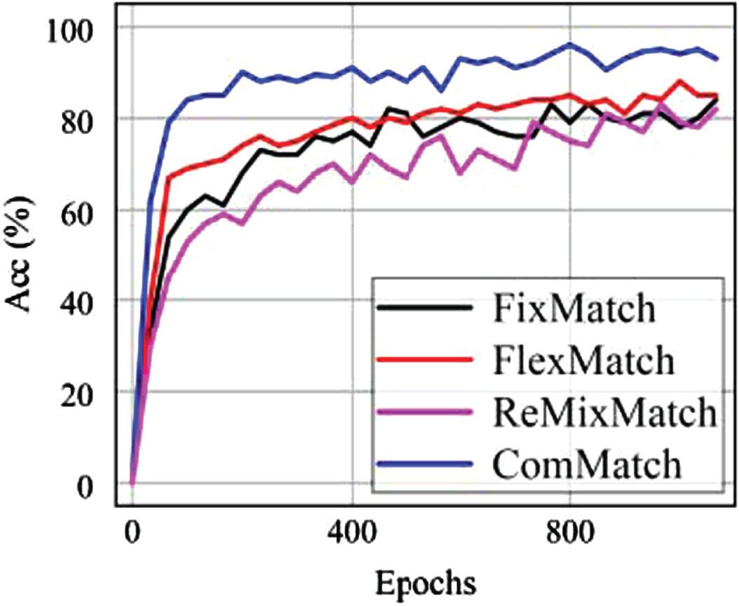
Comparison of accuracy of FixMatch, FlexMatch, ReMixMatch and ComMatch on CIFAR-10-40.

4.5 Ablation Study

We conduct ablation experiments to examine the effects of different components in ComMatch on the overall performance. We use the CIFAR-10 dataset with varying amounts of labeled data for the experiments. Negative learning and the predictive stability measure are evaluated using 4000 labeled samples, while dynamic thresholding is studied with only 40 labeled samples. The results are shown in Table 3.

Table 3
Ablation experiments of ComMatch on the CIFAR-10 dataset with two groups of labeled data: one with 1000 labeled samples and another with 4000 labeled samples

Components Error(1k) Error(4k)

Supervised 25.83 16.58

Without Predictive stability 19.27 12.36

Without Negative learning 9.97 4.23

Without Dynamic threshold 8.06 3.85

All 7.49 3.77

Components	Error(1k)	Error(4k)
Supervised	25.83	16.58
Without Predictive stability	19.27	12.36
Without Negative learning	9.97	4.23
Without Dynamic threshold	8.06	3.85
All	7.49	3.77

Negative learning We evaluate the effects of negative learning on training accuracy and speed. Our experiments reveal that ComMatch with negative learning outperformed the version without it on the CIFAR-10 dataset, which contains 4000 labeled samples. The version without negative learning has an error rate of 4.23%, which is higher than the version with negative learning that achieves an error rate of 3.77%. Notably, ComMatch with negative learning shows a faster convergence rate, reaching an accuracy of over 95.3% after just 500 iterations. These findings suggest that negative learning is a critical component of ComMatch that significantly enhances its performance and training efficiency.

Dynamic thresholding We find that ComMatch with dynamic thresholding achieves better performance when the amount of labeled data is limited. In particular, our experiments on the CIFAR-10 dataset with only 40 labeled samples show that ComMatch with dynamic thresholding significantly outperformed the version without it, reducing the error rate by 7.58%. The use of dynamic thresholding allows ComMatch to be more selective in assigning pseudo-labels to unlabeled samples, which in turn improves the accuracy of the model.

Stability predicting In our experiments, we find that incorrect pseudo-labeling becomes more prevalent as the amount of labeled data decreases. To address this issue, we incorporate a predictive stability measure in ComMatch, which leads to significant improvement in performance. Specifically, we observe that ComMatch without the predictive stability measure has a high error rate of 12.36%, which is 8.59% higher than the rate with the measure. To evaluate the reliability of the model, we plot the reliability graph in Fig. 4(b). The graph displays the difference between the true accuracy of the model and the expected confidence level in each probability interval. It is worth noting that the comparison in Fig. 4(a) shows that ComMatch has a much lower ECE value than FixMatch, and achieves good model calibration after incorporating the predictive stability measure, further demonstrating its superiority.

Fig. 4

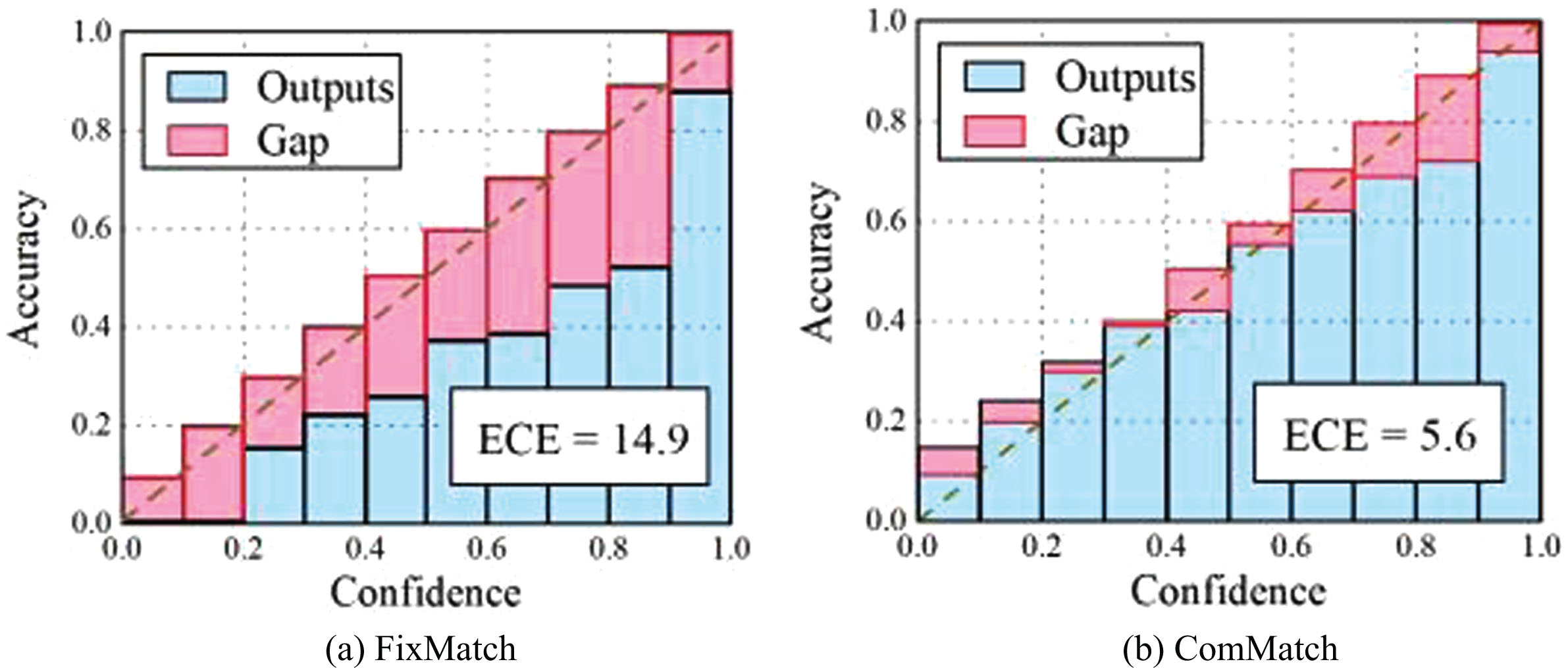
Comparison of reliability diagram between FixMatch and ComMatch. Reliability is shown on a CIFAR-100 dataset with 10,000 labeled data. The red boxes represent the difference between true accuracy and predictive accuracy, and the blue boxes represent true accuracy. (a) FixMatch (b) ComMatch.

The predictive stability measure helps to mitigate the risk of incorrect pseudo-labeling in ComMatch by evaluating the consistency of the predictions for each sample across multiple training iterations. Specifically, it measures the consistency of the predicted labels for each sample over multiple iterations and assigns a stability score based on the degree of consistency. Samples with lower stability scores are given lower confidence levels in the training process, which reduces the risk of incorrect pseudo-labeling. Overall, our results show that incorporating the predictive stability measure in ComMatch significantly improves model performance in scenarios with limited labeled data.

To further examine the effect of the predictive stability measure on model calibration, we conduct experiments with varying amounts of labeled data on different datasets and analyze the relationship between the ECE and predictive stability. The results reveal a negative correlation between ECE and predictive stability within a certain range, indicating that incorporating the predictive stability measure can significantly improve model calibration even with limited labeled data. Figure 5 graphically illustrates this relationship, demonstrating that ECE decreases as predictive stability increases, especially when predictive stability values are kept as small as possible (not exceeding 0.2).

Fig. 5

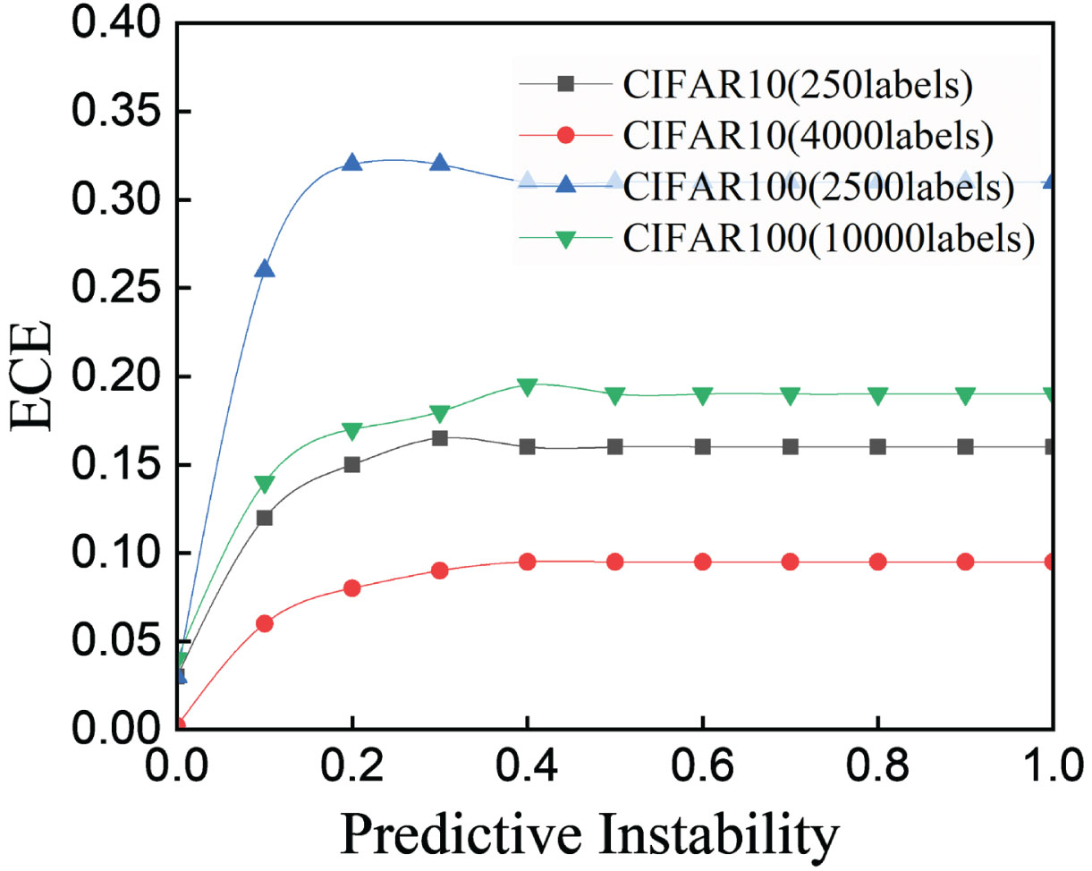
The relationship between predictive instability and the expected calibration error (ECE). Within the range of 0 to 0.2, as the instability decreases, meaning an increase in stability, the ECE score decreases. And within the range of 0.2 to 1, the ECE scores tends to level off.

5 Conclusion

In this paper, we present ComMatch, an SSL algorithm based on a consistent regularization approach combining negative learning, dynamic thresholding, and network predictive calibration, which achieves great results on many datasets while keeping the algorithm structure simple and improves the model’s robustness to noisy data. The unique feature of ComMatch is that it can guarantee training validity and accuracy through negative learning and ECE discrimination for a small number of labeled samples. We have reasons to believe that ComMatch can be applied to more complex and diverse scenarios in the future.

References

Bachman

, Alsharif

, Precup.

, Learning with Pseudo-Ensembles. 2014.

Belkin

, Niyogi

, Laplacian Eigenmaps and Spectral Techniques for Embedding and Clustering, Neural Information Processing Systems MIT Press, 2001.

Berthelot

, et al., Mixmatch: A holistic approach to semi-supervised learning, Advances in Neural Information Processing Systems 32 2019.

Berthelot

, et al., Remixmatch: Semi-supervised learning with distribution alignment and augmentation anchoring, arXiv preprint arXiv:1911.09785, 2019.

Chapelle

, Scholkopf

and Zien

, Semi-supervised learning (chapelle, o. et al., eds.; [book reviews], IEEE Transactions on Neural Networks 20(3) 2009.

Chen

, et al., Robust semi-supervised classification for imbalanced and incomplete data, Journal of Intelligent & Fuzzy Systems Preprint 1–17.

Chen

, et al., Semi-supervised learning with multi-head co-training, Proceedings of the AAAI Conference on Artificial Intelligence 36(6) 2022.

Chen

, et al., Big self-supervised models are strong semi-supervised learners, Advances in Neural Information Processing systems 33 2020.

Ekin Cubuk

, et al., Randaugment: Practical automated data augmentation with a reduced search space, Proceedings of the IEEE/CVF conference on computer vision and pattern recognition workshops 2020.

10.

Feng

, et al., Weakly-supervised semantic segmentation via online pseudo-mask correcting, Pattern Recognition Letters 165 2023.

11.

Gammerman

, Vovk

, Vapnik

, Learning by transduction.arXiv preprint arXiv:1301.7375, 2013..

12.

Grandvalet

and Bengio

, Semi-supervised learning by entropy minimization, Advances in Neural Information Processing Systems 17 2004.

13.

Guo

, et al., On calibration of modern neural networks, International conference on machine learning. PMLR, 2017.

14.

Geoffrey Hinton

, et al., Improving neural networks by preventing co-adaptation of feature detectors. arXiv preprint arXiv:1207.0580, 2012.

15.

Hwang

, et al., Entropy regularization for weakly supervised object localization, Pattern Recognition Letters 169 2023.

16.

Iscen

, et al., Label propagation for deep semi-supervised learning, Proceedings of the IEEE/CVF conference on computer vision and pattern recognition. 2019.

17.

Joachims

, Transductive inference for text classification using support vector machines, Icml 99 1999.

18.

Joachims

Transductive learning via spectral graph partitioning, Proceedings of the 20th international conference on machine learning (ICML-03) 2003.

19.

Kim

, et al., Nlnl: Negative learning for noisy labels, Proceedings of the IEEE/CVF international conference on computer vision 2019.

20.

Krizhevsky

, Hinton

Learning multiple layers of features from tiny images, 2009.

21.

Laine

, Aila

, Temporal ensembling for semisupervised learning. arXiv preprint arXiv:1610.02242, 2016.

22.

Lee

D-H.

, Pseudo-label: The simple and efficient semi-supervised learning method for deep neural networks, Workshop on Challenges in Representation Learning, ICML 3(2) 2013.

23.

, Xiong

, CH

Comatch: Semi-supervised learning with contrastive graph regularization, Proceedings of the IEEE/CVF International Conference on Computer Vision 2021.

24.

Liu

, et al., Deep metric transfer for label propagation with limited annotated data, Proceedings of the IEEE/CVF International Conference on Computer Vision Workshops 2019.

25.

Netzer

, et al., Reading digits in natural images with unsupervised feature learning. 2011.

26.

Odena

, Semi-supervised learning with generative adversarial networks. arXiv preprint arXiv:1606.01583, 2016.

27.

Rizve

M.N.

, et al., In defense of pseudo-labeling: An uncertainty-aware pseudo-label selection framework for semi-supervised learning. arXiv preprint arXiv:2101.06329, 2021.

28.

, et al., Variational autoencoder for deep learning of images, labels and captions, Advances in Neural Information Processing Systems 29 2016.

29.

Sajjadi

, Javanmardi

and Tasdizen

, Regularization with stochastic transformations and perturbations for deep semi-supervised learning, Advances in Neural inFormation Processing Systems 29 2016.

30.

Sohn

, et al., Fixmatch: Simplifying semi-supervised learning with consistency and confidence, Advances in Neural Information Processing Systems 33 2020.

31.

Tarvainen

and Valpola

, Mean teachers are better role models: Weight-averaged consistency targets improve semi-supervised deep learning results, Advances in Neural Information Processing Systems 30 2017.

32.

Wang

, et al., Freematch: Self-adaptive thresholding for semi-supervised learning. arXiv preprint arXiv:2205.07246, 2022.

33.

Xie

, et al., Self-training with noisy student improves imagenet classification, Proceedings of the IEEE/CVF conference on computer vision and pattern recognition 2020.

34.

Zagoruyko

, Komodakis

, Wide residual networks. arXiv preprint arXiv:1605.07146, 2016.

35.

Zhang

, et al., Flexmatch: Boosting semi-supervised learning with curriculum pseudo labeling, Advances in Neural Information Processing Systems 34 2021.

36.

Zhu

, Ghahramani

, Lafferty

J.D.

, Semi-supervised learning using gaussian fields and harmonic functions, Proceedings of the 20th International Conference on Machine Learning (ICML-03) 2003.

ComMatch: A semi-supervised learning classification algorithm based on model calibration

Abstract

Keywords

1 Introduction

2 Related work

2.1 Consistency regularization

2.3 Pseudo-labeling

2.4 Model Calibration

3 ComMatch

4 Experiments

4.1 Datasets

4.2 Implementation details

Table 1 List of ComMatch hyperparameters on the CIFAR-10, CIFAR-100 and SVHN datasets CIFAR-10 CIFAR-100 SVHN t p0 0.9 t n0 0.3 α epoch p 0.001 · (epoch - 1) α epoch n 10 - ( epoch 3 + 1 ) s p 0.05 s n 0.005 λ 1 μ 2 N c 10 lr 0.03 Batch s ize 64 Weight d ecay 0.0005 0.001 0.0005

CIFAR-10 and CIFAR-100

SVHN

References