A fuzzy rough granular ensemble learning based on the feature selection with chi-square 1

Abstract

Neighborhood granulation is a classical granulation method. Although it is adequate for clustering and classification tasks, its granules are more complex, and the data representation is binary. This paper proposes a new granulation method based on the neighborhood granulation. Firstly, a detailed definition of the granular form is given with fuzzy rough set theory. Then, a modified fuzzy rough discriminant function is proposed based on neighborhood systems. The samples are globally granulated on single features to construct granules and on multiple features to construct granular vectors. Also, a feature selection technique based on the Chi-square, which strikingly reduces the complexity of the fuzzy rough granular vectors, is introduced to address the disadvantage of the fuzzy rough granular vectors. An ensemble model structure is also proposed in the paper for the mixed nature of fuzzy rough granular vectors. The paper makes a detailed comparison between the fuzzy rough granulation and the neighborhood granulation. The results show that fuzzy rough granulation has higher computational efficiency and classification performance. Finally, a detailed comparison is made between the fuzzy rough granular ensemble model and various classical ensemble algorithms. The final results show that the fuzzy rough granular ensemble model has better robustness and generalization.

Keywords

Granular computing fuzzy rough granulation neighborhood granulation granular ensemble learning granular selection

1 Introduction

Classification problems have been one of the most challenging problems all the time [1, 2]. Since codes are human-predefined processes, they do not do better than humans when faced with unexpected and complex situations [3, 4]. A typical feature of human problem-solving is splitting the problem into multiple sub-problems when encountering a complex task. Then they utilize strong memory and similarity comparison capabilities to handle these sub-problems [5]. Due to the rising complexity of the problem, a single classification system can no longer meet the requirements for classification accuracy. As a result, ensemble learning has become a popular research area in recent years [9]. The construction of the ensemble model can be divided into two categories. The first category is constructed by parallel methods in which the relationships between the individual base learners are parallels, such as the Bagging algorithm and the Random Forest algorithm [10, 11]. The second category is built from sequential methods, in which the base learners are constructed sequentially, represented by algorithms such as the Boosting algorithm [12, 13].

Zadeh’s paper "Fuzzy sets and information granularity" marked the birth of fuzzy set theory. Zadeh argues that the concept of information granularity exists in many fields, such as interval operations in interval theory, uncertainty in control theory, etc. are manifestations of information granularity [6, 7]. Based on fuzzy set theory, Lin et al. published a paper called "Granular computing" in 1998, detailing the model of granular computing under binary relations, which marked the birth of granular computing [8]. Granular computing is an emerging multidisciplinary intersection theory that considers granular computing as an amalgamation of fuzzy set and rough set theory [14, 15]. The granules are the most fundamental element in constructing a granular computational model. To construct various granules, people can use metrics such as similarity and distance between features as the basis of granulation. In [16], Hu et al. proposed a way of Neighborhood Granulation defined by neighborhood relations, thus enabling granularity calculation in real space. In [17], Chen et al. proposed a fuzzy granulation based on single features combined with convolutional operations to optimize the weights to obtain a good classification performance. A primary characteristic of granular computing is the ability to reconstruct input patterns at a higher level of abstraction [18, 19]. As a result, granular computing can obtain more in-depth information. Based on this characteristic, classification models incorporating granular computing have also become another research hotspot [17, 20-22]. Therefore, combining the robustness of ensemble learning with the abstract level feature mining ability of granular computing is a field worth studying.

In the field of the granular classifier, Neighborhood Granulation is a widely used granulation method [23-25]. But the Neighborhood Granulation often faces some challenges. Firstly, granules generated from sample features and neighborhood systems are often too complex and take up too many resources in the computational phase of the model [23]. Secondly, since the Neighborhood Granulation divides samples into the poles of the Euclidean space, it isn’t easy to distinguish between similar but different samples. Finally, the Neighborhood Granulation classification performance tends to be poor in the range of minimax neighborhoods [24, 25]. Therefore, the optimization of neighborhood algorithms and improving the effectiveness of granular ensemble models are worth investigating. To deal with the complex and indistinguishable characteristics of neighborhood granules, a feature selection algorithm can be used to select the required granular kernels [26 , 35]. The complexity of neighborhood granules is mainly reflected in the repetitiveness and scale of granular characteristics. Filtering out irrelevant granular characteristics is a simple and intuitive way to reduce complexity. The chi-square test can be used for independence testing, which can effectively screen out irrelevant features that are independent of the label. Its computational efficiency also fits the theme of this study. To address the poor performance of granular decisions in minimax neighborhoods, the fuzzy membership function and the rough set theory are introduced in the granulation so that the features beyond the neighborhood are monotonically decreasing from 1 to 0 or vice versa. Experiments show that Fuzzy Rough Granulation performs far better than Neighborhood Granulation in minimax neighborhoods. The innovative nature innovation of the fuzzy rough granular ensemble learning is as follows:

The Fuzzy Rough Granulation is proposed to improve the model’s performance in minimax neighborhoods.

The introduction of a feature selection algorithm has dramatically improved the computational efficiency of the model.

Combining the characteristics of granular computing and ensemble learning allows the robustness of the model to be further improved.

The rest of the article is organized as follows. Section 2 describes the feature selection algorithm and the ensemble learning in detail. A detailed description of the theory and process of Fuzzy Rough Granulation is given in Section 3. The Fuzzy Rough Granular Ensemble Learning (FRGEL) is elaborated in Section 4, focusing on the model structure and the use of the Fuzzy Rough Granulation in the model. Section 5 gives an experimental analysis to verify the model’s advantages in several aspects. All the work is summarized in Section 6.

2 Related works

2.1 Feature selection with chi-square

The Chi-square statistic is a non-parametric statistical method, similar to all non-parametric statistics, and the method does not lose robustness due to changes in the sample distribution [26-28]. In the calculation, the chi-square test provides not only information on the observed differences between samples but also detailed information on the significant differences between exact categories. Specifically, χ² is calculated for all samples to discover the impact of features on the objective, which is then mapped to the relevance of the features on the decision according to the impact size [27, 28]. The formula of χ² is shown in equation (1).

$\sum χ_{i - j}^{2} = \frac{(O - E)^{2}}{E},$ (1) where O is the observed value, and E is the predicted value. The χ² is the cardinality of the interval under each feature. The ∑χ² is the sum of the cardinality over all intervals. In equation (1), the first thing to go for is frequencies under each interval, which requires adding up all the data’s rows and columns. The final result is the observed value O. Next, the expectation E is calculated, which indicates how the sample distribution would have changed if a feature was not present. The calculation formula is shown in equation (2).

$E = \frac{M_{R} * M_{C}}{n},$ (2) where E is the expected value in the interval, M_R denotes the row boundaries in the interval, M_C denotes the column boundaries in the interval, and n is the number of samples. Once the expected value E is calculated, the chi-squared value χ² within each interval can also be calculated using the following equation.

$χ^{2} = \frac{(O - E)^{2}}{E} .$ (3)

Due to the robustness of chi-square test, it is widely used in granular computing and machine learning. In [29], Xu et al. proposed a fuzzy priority discriminant made by an expert group, under which a cardinality test was used to obtain the priority vector of group decisions and finally obtained significant results. In [30, 31], the authors used the chi-square test as the basis for feature extraction. The method significantly reduced the complexity of the data, ultimately achieving better results on the target task.

2.2 Ensemble learning in granular computing

Classical machine learning algorithms such as SVM and LR perform well in specific scenarios. However, with the increasing complexity of the data scenarios, individual learners can no longer meet high robustness requirements. Consequently, multi-learner systems are gaining popularity. Due to the integration of the performance of multiple learners, ensemble learning tends to perform better in the face of the complex. At the same time, ensemble learning has gradually become popular in the field of granular computing because it tends to do processing and decision-making variety of highly abstract data.

In [32], Xia et al. proposed an ensemble learning combining the Naive Bayes, the maximum entropy algorithm, and the Support Vector Machine, combining the three ensemble methods and finally obtaining better classification results in the sentiment classification problem. In [33], the authors proposed a cosine similarity learner by learning the cosine similarity metric. Making a combination of multiple cosine similar learners ensures the diversity of the multi-classifier system and effectively improves the performance. The above works propose ensemble learning methods based on various metrics data for the high abstraction of data in their research areas, respectively, and use ensemble learning to achieve better results.

3 Fuzzy rough granulation

3.1 Granular representation

Let the sample space be IS = (X, A), where the sample set is X = {x₁, x₂, . . ., x_n} and the feature set is A = {a₁, a₂, . . ., a_m}. Given a sample x ∈ X, for any feature a ∈ A, v (x, a) ∈ [0, 1] denotes the value of sample x normalized over the feature a.

Definition 1. Given a sample space IS, for samples x_i, x_j ∈ U, a single attribute a ∈ A. Based on the definition provided by the author in [36], the Manhattan distance of x_i, x_j on attribute a is defined as: $s_{a} (x_{i}, x_{j}) = | v (x_{i}, a) - v (x_{j}, a) | .$ (4)

Definition 2. Given the sample space IS = (X, A) for samples x₁, x₂ ∈ X, feature set A_N ⊆ A, and given the neighborhood parameter σ which defines the discriminant parameter of the neighborhood system and the interruption parameter θ which defines the discontinuity value of the fuzzy rough membership function. The above two parameters are described in detail in section 3.2. The fuzzy rough affiliation function of sample x₁ to sample x₂ is defined as: $F (x_{1}, x_{2}, A_{N}, s_{a}, σ, θ | (x, a) \in IS) .$ (5)

If we define r = s_a, a ∈ A_N, then r represents the similarity between samples x₁ and x₂ under feature a. The smaller s_a,the more significant the similarity.

After doing the computation for two samples, a fuzzy rough set F_{s
_x} between the samples is generated, which is defined as shown below. $F_{s_{x}} = {\frac{r_{i}}{a_{i}} + \frac{r_{i + 1}}{a_{i + 1}} + . . . + \frac{r_{j}}{a_{j}}} .$ (6) where the + sign indicates not a sum in the mathematical sense, but a merging relationship. The r indicates the degree of affiliation of sample x₁ to x₂ on feature a ∈ A_N. Let $\frac{r_{i}}{a_{i}}$ be r_i, then: $F_{s_{x}} = {r_{i} + r_{i + 1} + . . . + r_{j}} .$ (7) Where r is called the fuzzy rough granular kernel, and this fuzzy affiliation function defines the similarity between the samples x₁ and x₂.

Definition 3. Given a fuzzy rough set F_{s
_x}, it represents the fuzzy roughness of the samples x₁ to x₂ on the feature set A_N = {a_i, . . ., a_j} ∈ A. Then according to the definition of rough set, the fuzzy rough set F_{s
_x} has the lower approximation set pos_F (x₁, x₂), the boundary domain bnd_F (x₁, x₂), and the negative domain neg_F (x₁, x₂). Then a fuzzy rough granule is defined as follows:

$\begin{matrix} g_{FR} & = {{pos}_{F} (x_{1}, x_{2}) + {bnd}_{F} (x_{1}, x_{2}) + {neg}_{F} (x_{1}, x_{2})} \\ = {{pos}_{F} (x_{1}, x_{2}) ⋃ {bnd}_{F} (x_{1}, x_{2}) ⋃ {neg}_{F} (x_{1}, x_{2})} \end{matrix}$ (8) A fuzzy rough granule is a rough set between samples based on a fuzzy affiliation function.

Definition 4. Given a sample space IS = (X, A), for a sample x ∈ U, a feature set A_N = {a_i, . . ., a_j} ∈A, a neighborhood parameter σ and an interruption parameter θ. According to the inter-sample fuzzy rough affiliation function F, the fuzzy rough set generated by the sample x concerning sample set X is F_{s
_X}, which is shown as follows: $\begin{matrix} F_{S_{x}} & = {F_{s_{x_{1}}} + F_{s_{x_{2}}} + . . . + F_{s_{x_{n}}}} \\ = {{r_{x_{1}, i} + . . . + r_{x_{1}, j}} + . . . + {r_{x_{n}, i} + . . . + \\ r_{x_{n}, j}}} \end{matrix}$ (9) The result is a concatenation of multiple fuzzy rough sets. This fuzzy rough set is converted to fuzzy rough grain form according to Definition 3, and the result is as follows: $\begin{matrix} G_{FR} (x, X) & = {g_{FR} (x, x_{1}) + . . . + g_{FR} (x, x_{n})} \\ = {g_{FR} (x, x_{1}) ⋃ . . . ⋃ g_{FR} (x, x_{n})} \\ = {g_{FR} (x, x_{1}), . . ., g_{FR} (x, x_{n})} \end{matrix}$ (10) Call G_FR (x, X) is the fuzzy rough granular vector of the sample x to the sample set X.

3.2 Fuzzy rough membership function

Unlike the Neighborhood Granulation, the fuzzy rough affiliation function is introduced to the neighborhood discriminant stage to replace the original neighborhood discriminant function. The following section shows the construction process of the fuzzy rough affiliation function and the granular vector by example.

Traditional neighborhood algorithms assign 0 to values beyond the neighborhood size, which indicates that two samples are not adjacent to each other under a single feature; assign a value of 1 to the value less than or equal to the neighborhood threshold, which indicates that two samples are adjacent under a single feature [16]. As the traditional neighborhood algorithm has only two discriminant values, it will generate the same number of discriminant domain according to it. The discriminant formula is shown in equation (11) [23]. $y = {\begin{matrix} 0, s_{a} > σ \\ 1, s_{a} \leq σ \end{matrix}$ (11)

The general situation of the neighborhood discriminant function under the two features is shown in Fig. 1. The left figure shows the image of the discriminant function, the middle figure shows its value domain distribution, and the right figure shows the discriminant domain generated in the sample space for the two-dimensional sample neighborhood discriminant function. It can be seen that the neighborhood discriminant function divides a square discriminant domain around the sample.

Fig. 1

Neighborhood discriminant function.

Since the discriminant function will only produce discrete values of 0 and 1, the samples will be rigidly partitioned into two interval levels under a single feature. Suppose there is a sample set X = {x₁, x₂} in the sample space IS and the feature set is A = {a₁, a₂, a₃}, where x₁ = [0.2, 0.5, 0.7] and x₂ = [0.4, 0.6, 0.4]. According to Definition 1, the Manhattan distances of sample x₁ and sample x₂ for sample set X are illustrated in Table 1. Where d_i,i ∈ [1, 6] represents the Manhattan distance between sample x_j,j ∈ [1, 2] and sample set {x₁, x₂} under feature set A.

Table 1

Manhattan distances for the sample

Samples	d ₁	d ₂	d ₃	d ₄	d ₅	d ₆
x ₁	0	0	0	0.2	0.1	0.3
x ₂	0.2	0.1	0.3	0	0	0

Let the neighborhood parameter σ = 0.2, and according to Equation (11) , the granulation results of sample x₁ and sample x₂ are shown in Table 2.

Table 2

Neighborhood granular vectors

Samples	d ₁	d ₂	d ₃	d ₄	d ₅	d ₆
x ₁	1	1	1	1	1	0
x ₂	1	1	0	1	1	1

According to Table 2, it is easy to know that since 0.2 is chosen as the neighborhood discriminant parameter, the granulation results of the two samples for feature a₃ are distributed to the poles of the interval. It is then possible to distinguish samples x₁ and x₂ based on the granular kernel r₃ and the granular kernel r₄. a feature that makes the Neighborhood Granulation perform better on linear classifiers. This property makes the Neighborhood Granulation will get better performance on linear classifiers. Correspondingly, for sample x₁, the kernels {r₁, r₂, r₃, r₄, r₅} are positive domain kernels and r₆ are negative domain kernels. However, As the number and variety of samples are on the rise, there are many continuous and discrete values in the samples. Then it is difficult to satisfy the diversity by neighborhood division alone. This is because when the values under a certain feature are clustered in a certain interval, it can lead to difficulty in picking the appropriate neighborhood parameters to discriminate these values. If the neighborhood parameters are chosen to be minor, the diversity in the large interval is ignored, and vice versa.

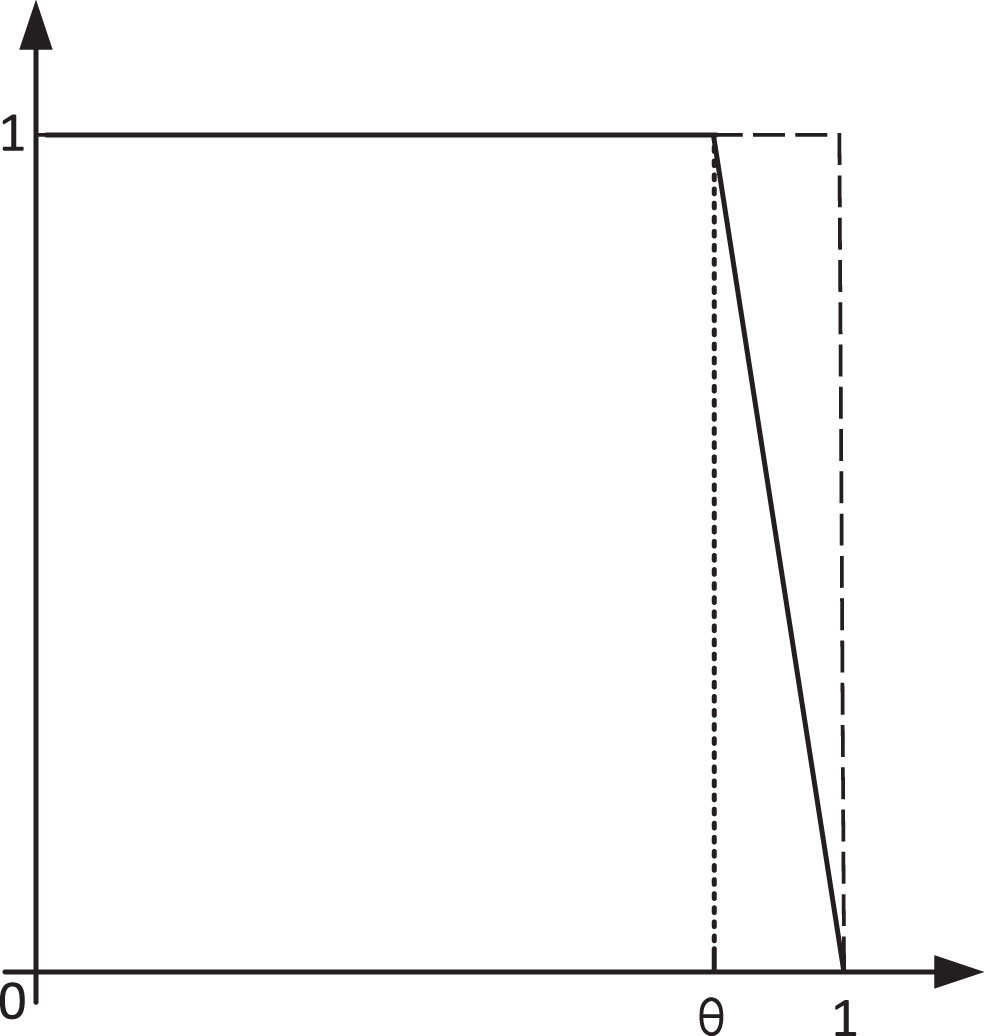
Therefore, a new discriminant method is needed to preserve the neighborhood system’s properties while keeping the values outside the neighborhood from being rigidly classified to zero. Here the fuzzy rough slope affiliation function is introduced to discriminate the points outside the neighborhood. The points at the neighborhood boundary and inside are classified as 1. The decreasing slope affiliation function judges the points outside the neighborhood to the sample space boundary. When σ > 0, a line through (σ, 1) and (1, 0) is used as the basis for judgment. The discriminant is shown in Equation (12). The unidirectional fuzzy rough affiliation function is shown in Fig. 4.

$y = {\begin{matrix} \frac{1}{σ - 1} s_{a} - \frac{1}{σ_{1}}, σ < s_{a} \\ 1, s_{a} \geq σ \end{matrix}$ (12)

According to Fig. 2, a smaller neighborhood can be chosen because of the monotonically decreasing nature of the value of the affiliation function outside the neighborhood. This way, it is possible to preserve the properties within the neighborhood and assign different values to objects beyond the scope of the neighborhood. Then, according to the properties within the neighborhood, the discriminative domain can be categorized into three parts, which are the positive domain belonging to the neighborhood, the boundary domain outside the neighborhood to the boundary of the sample space, and the boundary of the sample space, i.e., the negative boundary. In other words, the fuzzy rough affiliation function divides the neighborhood discriminant domain from the original fuzzy positive and negative domains into positive, boundary, and negative domains with rough properties. Where the values in the positive domain are considered to be perfectly similar, the values in the boundary domain are considered to have different degrees of similarity, and the values in the negative boundary are considered entirely dissimilar [16]. For example, x₂ and x₃ in the right figure, are both in the boundary domain of the sample x and have affiliations of 0.8 and 0.7, respectively.

Let the neighborhood parameter σ = 0.1, and according to Equation (12) , the granulation results of sample x₁ and sample x₂ are shown in Table 3. As is described in Table 3, the Fuzzy Rough Granulation produces a mutually unequal set of granular kernels R = {r₁, r₃, r₄, r₆}. The set R has more kernels than Table 2, so it can express more information, making the points beyond the neighborhood not monotonically 0-valued, but continuous values with diversity. According to the Definition (2), (3) and (4), {r₂, r₅} is the positive domain kernel, and {r₁, r₃, r₄, r₆} is the boundary domain kernel. The fuzzy rough granular vector generated by the sample x₁ against the sample set X = {x₁, x₂} is G₁.

Fig. 2

The unidirectional fuzzy rough membership function.

Table 3

Unidirectional fuzzy rough grain vectors

Samples	d ₁	d ₂	d ₃	d ₄	d ₅	d ₆
G ₁	1	1	1	0.889	1	0.778
G ₂	0.889	1	0.778	1	1	1

However, it is not enough to introduce only a unidirectional affiliation function. As the values of the neighborhood parameters increase, the gradient of the affiliation function derived from the boundary points also becomes larger. This means that the affiliation function becomes steeper and steeper. As shown in Fig. 3, when the neighborhood parameters are increased to within the huge point region, the values within the huge neighborhood will change too fast due to the excessive gradient of the affiliation function. Let the σ = 0.8, and according to Equation (12) , the granulation results of sample x₁ and sample x₂ are shown in Table 4.

Fig. 3

Decreasing fuzzy rough discriminant function.

Table 4

Unidirectional fuzzy rough grain vectors in the extreme area

Samples	d ₁	d ₂	d ₃	d ₄	d ₅	d ₆
G ₁	1	1	1	1	1	1
G ₂	1	1	1	1	1	1

As can be seen from Table 4, the unidirectional affiliation function degenerates into a neighborhood discriminant function when the parameters fall into a extreme area.

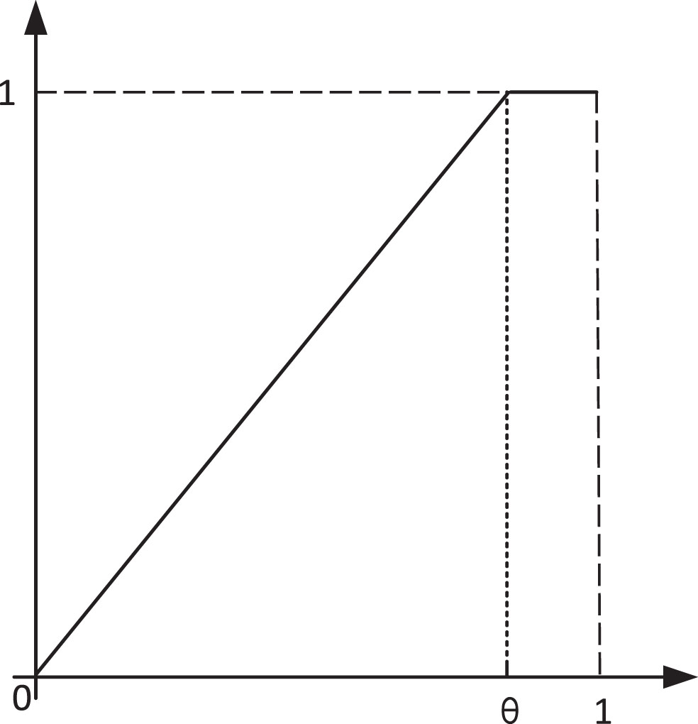
According to the neighborhood property, the neighborhood will divide the grain kernels with similar values into one set, and those outside the neighborhood belong to another set. Therefore, the granular kernels outside the neighborhood can be set to 1, and the granular kernels inside the neighborhood are assigned with a monotonically increasing affiliation function. The slope function is determined by the origin point (0,0) and the boundary point (σ,1). The discriminant is shown in equation (13), and the function image is shown in Fig. 4.

Fig. 4

Increasing fuzzy rough discriminant function.

$y = {\begin{matrix} \frac{1}{σ} s_{a}, s_{a} < σ \\ 1, s_{a} \geq σ \end{matrix}$ (13)

Let the σ = 0.8, and according to Equation (13) , the granulation results of sample x₁ and sample x₂ are shown in Table 5.

Table 5

Fuzzy rough granular vectors in the extreme area

Samples	d ₁	d ₂	d ₃	d ₄	d ₅	d ₆
G ₁	0	0	0	0.25	0.125	0.375
G ₂	0.25	0.125	0.375	0	0	0

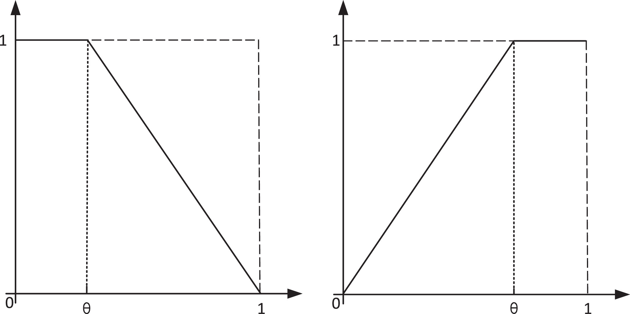
As can be seen from Table 5, the granular kernels can still maintain diversity when the neighborhood parameters are large, which is the opposite of the results in Table 4. $y = {\begin{matrix} f_{1} = {\begin{matrix} \frac{1}{σ - 1} s_{a} - \frac{1}{σ - 1}, σ \leq s_{a} \\ 1, s_{a} < σ \end{matrix}, 0 < σ \leq θ \\ f_{2} = {\begin{matrix} \frac{1}{σ} s_{a}, s_{a} < σ \\ 1, s_{a} \geq σ \end{matrix}, σ > θ \end{matrix}$ (14)

According to Fig. 4, the values outside the great neighborhood are assigned to 1. The values inside the great neighborhood are assigned with an increasing affiliation function whose slope is much smaller than before. This preserves the properties of the Neighborhood Granulation while giving the kernels diversity within the neighborhood. Combining the fuzzy affiliation function of the minimax neighborhood and setting the intermittent parameter θ as the junction point between the minimax neighborhood, the final obtained fuzzy rough discriminant function is shown in Equation (14), and the function is shown in Fig. 5.

Fig. 5

The fuzzy rough discriminant function.

4 Fuzzy rough granular ensemble learning

4.1 Model structure

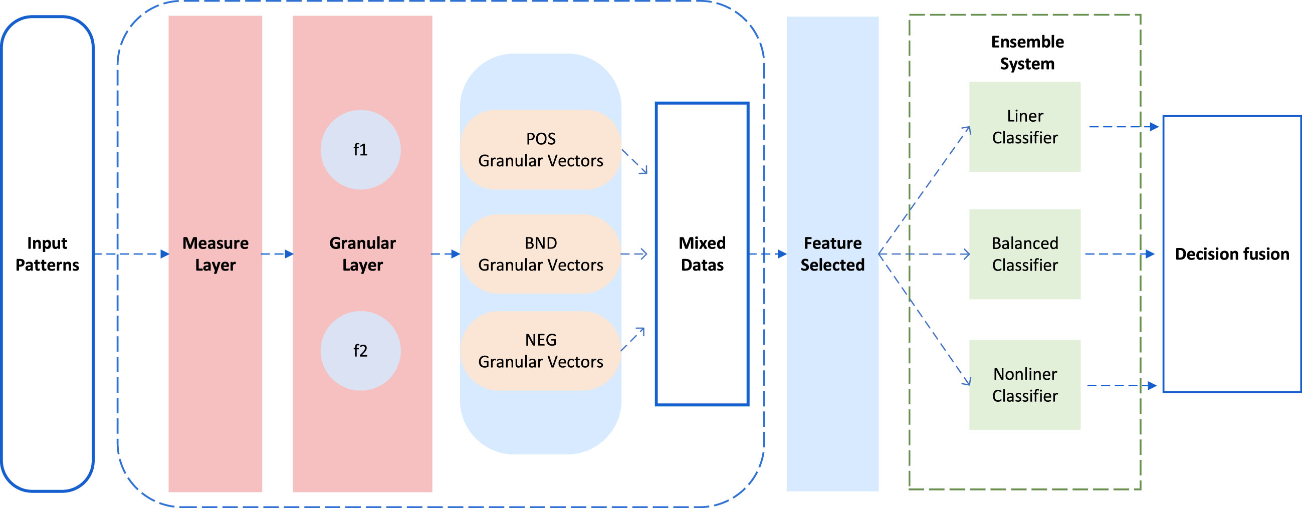
Unlike the discrete binary values that the neighborhood discriminant function will only produce, the fuzzy rough discriminant function will produce a series of mixed data. One part of the data will inherit the properties of the neighborhood discriminant function, producing a set of discrete values with small variations, while the other part will be continuous values with diversity. For the Neighborhood Granulation, linear classifiers tend to have better results because the final granular vectors are distributed across the vertices of the high-dimensional space. However, the linear classifier cannot meet the requirement of high classification accuracy for continuous values that will generate category crossover in the sample space. Therefore, for fuzzy rough granules with mixed data, both linear classifiers are needed for their powerful classification of discrete values, and nonlinear classifiers are needed to handle continuous values that tend to produce data crossover. In summary, Ensemble Learning (EL) is an excellent idea for solving the problem. A series of linear and nonlinear classifiers can be an ensemble for linear and nonlinear data, and a decision fusion mechanism can be introduced to make the final decision. The basic structure of the model is shown in Fig. 6.

Fig. 6

The granular ensemble learning model.

First, the normalized sample is input to the measure layer to generate the measure matrix M. The measure matrix M represents the variability of each sample. According to equation (4), the sample under a certain characteristic is greater in case of the value of the M is larger. Next, the measurement matrix is fed to the granulation layer. The granulation layer selects the appropriate discriminator for the measurement matrix based on the neighborhood parameters and intermittent parameters that enter along with the measured matrix. The output of this layer is three set vectors: the positive domain granular vectors posGs, the boundary domain granular vectors bndGs, and the negative domain granular vectors negGs. These granular vectors are stitched and combined to form fuzzy rough granular vector FRGs which contain mixed data.

After the FRGs are input to the feature selection layer, the correlation χ² between each granular kernel and the decision is first calculated according to Equations (1) and (2). Then we make a feature selection of FRGs in order according to the input threshold and select the set of granular kernels that have more influence on the decision. And finally, the new fuzzy rough granular vectors FRGNs are output.

For the FRGNs with mixed data, a combination of linear classifier, nonlinear classifier, and balanced classifier is proposed in this paper in the ensemble system module. Since both posGs and negGs are discrete data of 1 and 0, the samples will be distributed across the vertices of the high-dimensional space. Aiming at the characteristic, linear classifiers such as Linear Regression (LR), Support Vector Machines (SVM), etc., with better performance and faster computational efficiency, are used. On the contrary, in the bndGs, the data are all continuous values that do not contain 0 and 1. Since these continuous values are divided by neighborhood parameters, these values produce category stacking or crossover in the sample space. For these values, linear classifiers no longer obtain sufficiently good decision performance, so nonlinear classifiers such as the Gaussian Mixture Model (GMM) are used for decision discrimination. Finally, a balancer is combined, usually choosing an ensemble algorithm such as the Random Forest (RF), Boosting, etc. In this way, the classification results of linear or nonlinear classifiers can be augmented according to the powerful performance of the balancer on nonlinear data versus linear data. Finally, the decision granules output from each base learner is fused to discriminate.

4.2 Algorithm

In contrast to traditional Ensemble Learning (EL), Fuzzy Rough Granular Ensemble Learning (FRGEL) requires a granulation and feature selection step before construction, and the granular decisions need to be fused in the final decision.The specific flow of the algorithm is as follows.

Algorithm 1 Construction algorithm of FRGEL

Input:the sample set; Y: the label set; σ: the neighborhood parameter; θ: the intermittent parameter; r: the rule algorithm; k: the threshold values for feature selection.

Output: the Evaluated Set.

1: X is the input to the measure layer, and M is the output according to the measure formula, then go to 2;

2: M is the input granulation layer, go to 3;

3: if σ ≤ θ

4: M is input to discriminator f1 to calculate fuzzy rough set FRSs, go to 8;

5: else

6: M is input to discriminator f2 to calculate fuzzy rough set FRSs, go to 8;

7: end if

8: FRSs are spliced to construct the fuzzy rough granular vectors FRGs, go to 9;

9: FRGs are input to the selection layer, and the granular kernel is calculated according to r and k. The new fuzzy rough granular vectors FRGNs are output, go to 10;

10: for i = 0; i < 3; i++ do

11: Construct the i-th base classifier based on FRGNs, go to 12;

12: Construct the decision granule g base on the i-th base classifier;

13: end for

14: All decision granules are input to the fusion module to construct the final decision d, go to 15;

15: Compare the final decision d with the label y and outputting Evaluated Set;

In the construction process of FRGEL, time consumption is mainly concentrated in two parts: granulation process and integration processing. In the granulation process, since it is necessary to perform feature-level global fuzzy rough granulation on the original data, the time efficiency in this process is O (n²). Correspondingly, the space complexity at this time is also O (n²). Then, the granulated data is subjected to granule selection. Assuming that the proportion of granule selection is k, the space complexity of the particles after selection is O (kn²). Although in most cases O (kn²) is greater than O (n), after reasonable selection, the data size after granule selection will be much smaller than before. In the integration processing stage, due to parallel operation of three basic classifiers, the calculation time efficiency is determined by the basic classifier with the highest time complexity, that is, MAX {O (c) , c ∈ C}.

5 Experiment analysis

In this chapter, experiments adopt twenty Kaggle and UCI datasets, which the specific information of the datasets is shown in Table 6. Three experiments were implemented on the model to test the effectiveness of the algorithm.The experiment section verifies the three innovative points proposed in the first section. Section 5.1 conducted a comparative experiment between NG and FRG, which verified the effectiveness of fuzzy rough granulation in minimax neighborhoods. Section 5.2 compared the effect before and after granular selection, verifying the efficiency of the method. Section 5.3 conducted a comprehensive comparison of fuzzy rough granular ensemble learning, verifying the superiority of the model.

This section covers various comparison algorithms, including Random Forests (RF), AdaBoost [37], Bagging, HistGradientBoosting (HGB) [38], GradientBoosting (GB) [39], and XGBoost [40]. Their parameter settings are as follows. Among them, the tree of RF is constructed based on entropy, and the number of base estimators is 100; the estimator category of AdaBoost is decision tree, the learning rate is 1.0, the construction algorithm is SAMME.R, and the number of base estimators is 50; the base estimator of Bagging is a decision tree, and the number of base estimators is 10; the loss function of HGB is cross-entropy loss, the learning rate is 1.0, and the maximum number of iterations is 100 times; the loss function of GB is log loss, the learning rate is 1.0, there are 100 estimators, and the loss function is mse; XGBoost’s feature sampling ratio is 0.7, the objective function is softmax, the learning rate is 0.3, and the number of base estimators is 100. All experimental results from this chapter are achieved by ten-fold cross-validation with four decimal places retained.

Table 6
Datasets

Datasets Dimension Categories Number of samples

breast cancer 30 2 569

mobile 20 4 2000

diabetes 8 2 768

heart 13 2 269

seed 7 4 209

star 24 7 240

glass 9 6 213

blood 4 2 747

leaf 14 30 339

iris 4 3 150

raisin 7 2 900

acoustic 50 4 400

gender 22 3 4745

HCV 12 5 611

shill 10 2 6321

ILPD 10 2 578

wine quality 21 10 5000

yeast 8 10 1484

waveform 21 3 5000

Debrecen 19 2 1150

Datasets	Dimension	Categories	Number of samples
breast cancer	30	2	569
mobile	20	4	2000
diabetes	8	2	768
heart	13	2	269
seed	7	4	209
star	24	7	240
glass	9	6	213
blood	4	2	747
leaf	14	30	339
iris	4	3	150
raisin	7	2	900
acoustic	50	4	400
gender	22	3	4745
HCV	12	5	611
shill	10	2	6321
ILPD	10	2	578
wine quality	21	10	5000
yeast	8	10	1484
waveform	21	3	5000
Debrecen	19	2	1150

5.1 Comparison of NG and FRG

On the basis of the above analysis and study, the effects of the fuzzy rough granulation and the neighborhood granulation on sample distribution and classification are further compared, where the sample distributions were compared on the gender, mobile and seed datasets with different neighborhood parameters.

The classification effects of the two granulation methods were compared on six datasets, such as breast cancer and mobile. The specific classification effects are shown in Table 7 and Fig. 7. where σ is the neighborhood parameter, Origin is the original data in Table 7, FRG is the fuzzy rough granular vector, and NG is the neighborhood granular vector. The experimental results are obtained by the Random Forest.

Fig. 7

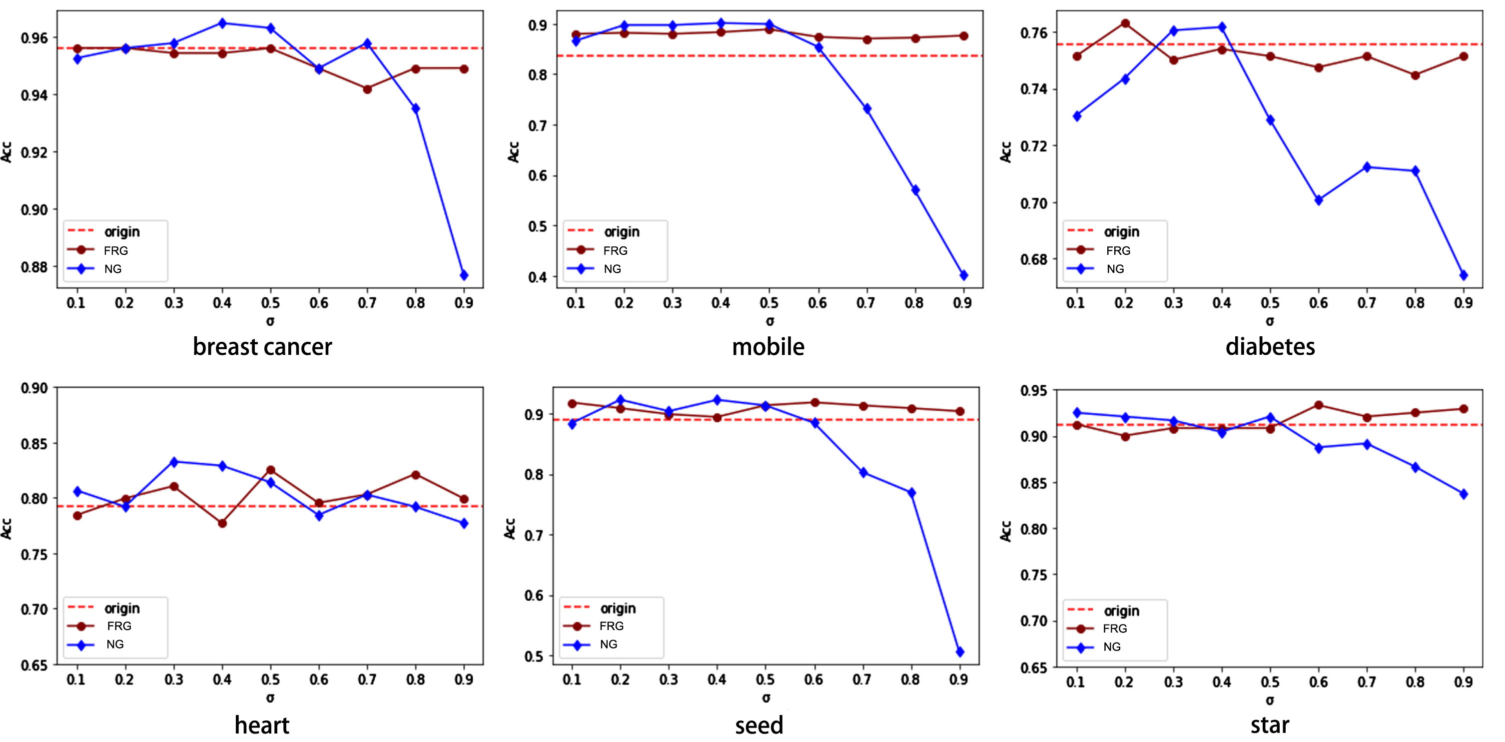
Comparison of classification effects between FRG and NG.

Table 7

The result of FRG and NG

Datasets	Origin	FRG	NG
breast cancer	0.9596±0.0008	0.9561±0.0008	0.9631± 0.0004
mobile	0.8825±0.0006	0.8915±0.0002	0.9015±0.0002
diabetes	0.7474±0.0025	0.7603±0.0040	0.7603±0.0025
heart	0.7956±0.0060	0.8254±0.0062	0.8328±0.0010
seed	0.8986±0.0089	0.9186±0.0046	0.9228±0.0060
star	0.9125±0.0033	0.9333±0.0060	0.9208±0.0032
Average	0.8570±0.0037	0.8809±0.0036	0.8836±0.0022

From Fig. 7 and Table 7, it can be seen that both FRG and NG have better classification effects on the optimal neighborhood than the original data, with an average improvement of about 0.025. Especially, the classification results of FRG on all neighborhood parameters are symmetrically distributed and have no significant decreasing trend. However, the classification results of NG mostly decrease with the increase of neighborhood parameters. The results revealed that the variation on the neighborhood parameters is subtly less effective on FRG, which makes FRG perform better than NG in the minimax neighborhood.

Figure 8 shows the data distribution of NG and FRG on the Gender and Mobile datasets. The left figure shows the distribution result of NG, and the right figure shows the distribution result of FRG. The decimal on the left side of the figure represents the value of the neighborhood parameter σ. As can be seen from the figure, the distribution of NG changes considerably with the expansion of the neighborhood parameters on these datasets. In contrast, FRG will maintain a similar distribution, and its distribution will not respond significantly to changes in the neighborhood parameters. Therefore, FRG are insensitive to the changes in the neighborhood parameters and have stronger robustness.

Fig. 8

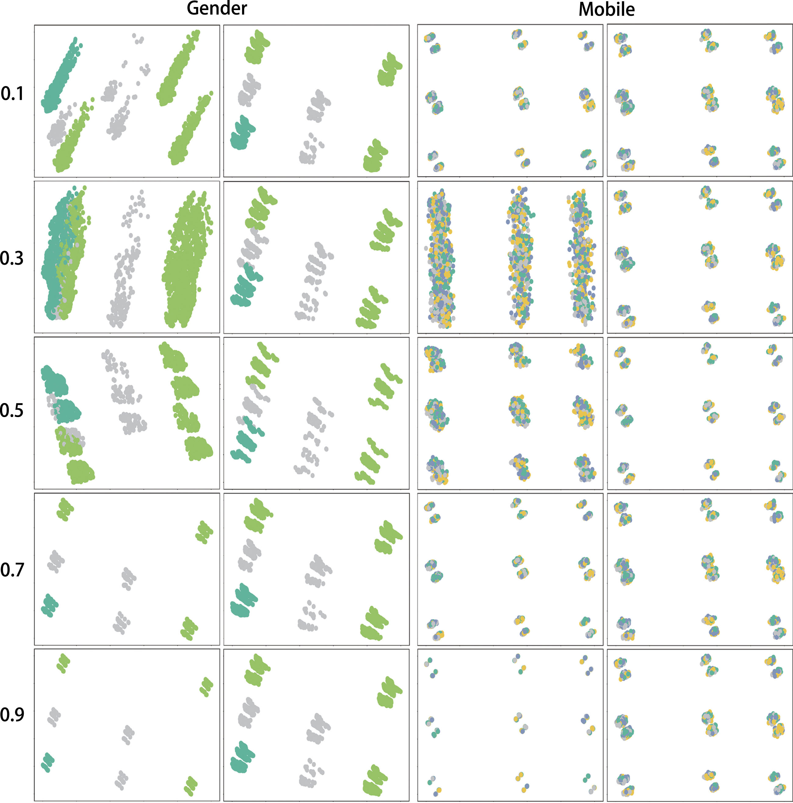
Comparison of the distribution of FRG and NG.

5.2 Granular selection

A major drawback of the neighborhood algorithm is that it will expand the latitude of the sample with high complexity, which will cause the algorithm to end up spending a lot of computational cost on decision-making. According to Tables 2-5, it can be seen that in the process of granulation, many refuted features are generated, such as: {r₁, r₂, r₄, r₅} in Table 2 and {r₂, r₄} in Table 3. According to these granular kernels, there is no way for the algorithm to calculate which one the final decision actually belongs to.

Since the distribution of the samples depends mainly on its feature set, too many granular kernels will not only increase the computational burden of the model but also interfere with the model’s decision-making. Too many features can make it difficult for the model to find the appropriate decision boundary, producing overfitting. Therefore, it is necessary to make a feature selection on the granular vectors, which is beneficial to combine the properties of the granular calculation with the advantages of the feature selection algorithm.

This experiment is based on the Chi-square algorithm, which calculates the correlation between the FRGs and the decision based on Equations (1) and (2) and then makes multiple feature selections for the granular kernel based on the correlation. The effect of feature selection on the mobile dataset is shown in Fig. 9. Where σ is the neighborhood parameter, k is the approximate proportion of selected features, acc is the classification accuracy, and the interruption parameter θ = 0.5. At σ = 0.4 and k = 1, the various categories of FRGs are stacked together in a hierarchy, and at this point, the samples are not evenly distributed in the sample space, although they possess a certain degree of differentiability. Even so, they still have a higher degree of accuracy than the original data. When σ = 0.4 and k = 0.125, it can be seen from the rightmost graph that the parameter k takes values reaching near the extreme value point. In this case, although the FRGs follow the original distribution of the sample, the FRGs have more distribution results in areas where the original samples are rarely distributed, so the FRGs are more uniformly distributed than the original sample. At this point, the classification accuracy of the sample reached 0.9275, which is about 0.09 higher than the classification accuracy of the original data.

Fig. 9

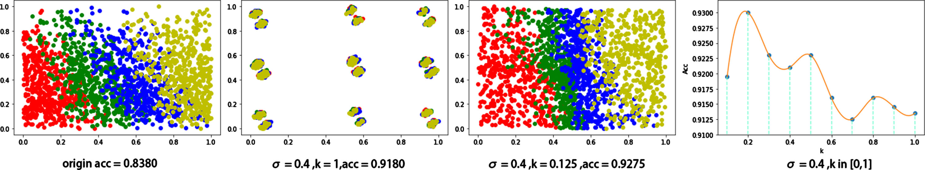
Effect of feature selection of FRG on mobile.

Based on the above experiments, a detailed comparison of the original data as well as the NG and the FRG after feature selection was made on six datasets, such as Glass, Blood, and Leaf, respectively. The underlying model for the experiments is the FRGES model proposed in this paper. The comparison results are shown in Fig. 10 and Table 8. Among them, Table 8 shows the comparison results before and after feature selection. Figure 10 shows the effect of the two granulation methods on each neighborhood parameter.

Fig. 10

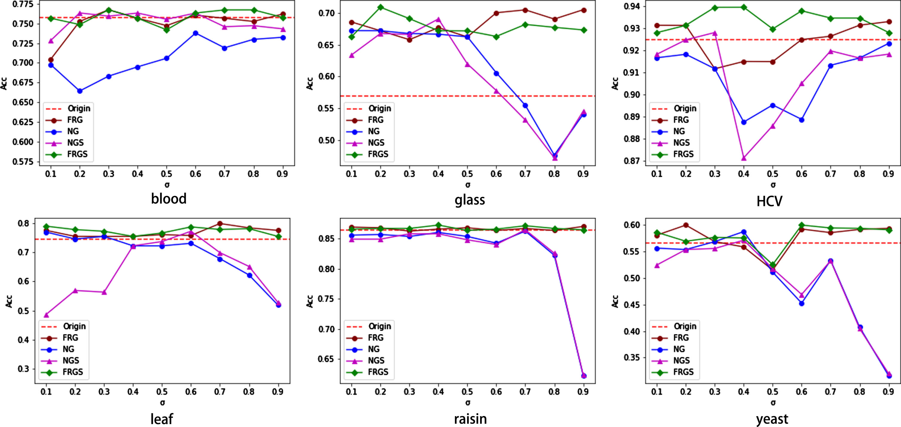
Comparison of multi-neighborhood feature selection.

In Table 8, NGS and FRGS indicate the classification accuracy (mean ± var) of the NG and the FRG after optimal feature selection, respectively, and k indicates the proportion of feature selection. Enhanced classification results of FRG demonstrate feature selection is an advisable method. Among them, the improvement was more obvious in HCV, with an improvement of about 1.47% in classification accuracy. Also, there is an improvement of about 0.5% on glass and raisin. A significant improvement of FRGS over FRG is the reduction of variance. The variance of FRGS was, on average, about 0.26% lower than FRG on the six data sets in the table. Overall, both the NG and the FRG are better than the original data, with an average of about 1.62% and 3.63% higher, respectively. Relatively, the FRG improves the classification accuracy by about 1.75% on average over the NG and also has a lower mean squared error. In summary, it can be seen that the FRG has higher classification accuracy and robustness than the NG.

Table 8

The result of FRG and NG

Datasets	Origin	NG	NGS	FRG	FRGS	k
glass	0.5969±0.0124	0.6721±0.0125	0.6905± 0.0097	0.7049±0.0157	0.7097±0.0124	0.2
blood	0.7578±0.0006	0.7377±0.0011	0.7631±0.0049	0.7672±0.0112	0.7672±0.0045	0.3
leaf	0.7463±0.0023	0.7700±0.0043	0.7729±0.0062	0.7994±0.0048	0.7932±0.0021	0.3
HCV	0.9247±0.0004	0.9231±0.0004	0.9280±0.0006	0.9329±0.0006	0.9476±0.0002	0.3
raisin	0.8644±0.0013	0.8620±0.0013	0.8578±0.0011	0.8689±0.0017	0.8722±0.0014	0.4
yeast	0.5644±0.0005	0.5866±0.0011	0.5704±0.0026	0.5988±0.0013	0.5988±0.0009	0.3
Average	0.7424±0.0029	0.7586±0.0035	0.7637±0.0042	0.7787±0.0061	0.7812±0.0035	0.3

Figure 10 shows the classification effects of the FRG and the NG before and after the feature selection exercise and compares them with the original data. It can be seen that the FRG has a clear advantage in blood, glass, HCV, and raisin datasets, and the classification results are superior to other algorithms under most neighborhood parameters. In contrast, the NG performs better in certain neighborhoods, locally obtaining a performance that exceeds that of other algorithms, as in the case of σ = 0.4 in glass and σ = [0.2,0.4] in blood. However, on most data sets, the results of the NG show a monotonically decreasing trend with increasing neighborhood parameters. So, the algorithm is sensitive to parameters, and the variation of parameters makes the classification effect of the NG less stable than that of the FRG. The FRGS has more efficient computational efficiency and more significant and stable classification results than the NG and NGS.

5.3 Comprehensive comparison

In this section, the classification results of the Fuzzy Rough Granular Ensemble Learning (FRGEL) are compared in detail with those of the traditional ensemble algorithm on 16 datasets. The specific algorithms compared are RF, Adaboost, Bagging, HGB, GB, and XGBoost. The specific results are shown in Table 9.

Table 9
Results of FRGEL and EL on 20 datasets

Datasets RF Adaboost Bagging HGB GB XGBoost FRGEL

breast cancer 0.9596±0.0008 0.9491±0.0008 0.9771±0.0013 0.9684±0.0003 0.9632±0.0003 0.9789±0.0006 0.9754±0.0003

mobile 0.8825±0.0006 0.7210±0.0018 0.8665±0.0005 0.9120±0.0002 0.9110±0.0003 0.9205±0.0002 0.9300±0.0003

diabetes 0.7474±0.0025 0.7527±0.0033 0.7683±0.0036 0.7344±0.0014 0.7591±0.0029 0.7357±0.0019 0.7773±0.0008

heart 0.7956±0.0060 0.7845±0.0073 0.7698±0.0097 0.8030±0.0047 0.8178±0.0045 0.8141±0.0052 0.8661±0.0055

seed 0.8986±0.0089 0.6733±0.0100 0.9229±0.0046 0.8983±0.0114 0.9233±0.0037 0.9133±0.0060 0.9318±0.0052

star 0.9125±0.0033 0.6750±0.0206 0.9125±0.0050 0.9000±0.0098 0.8958±0.0053 0.9417±0.0032 0.9292±0.0024

glass 0.6995±0.0096 0.3900±0.0224 0.6065±0.0109 0.6665±0.0119 0.6476±0.0188 0.6903±0.0186 0.7097±0.0124

blood 0.6643±0.0196 0.7873±0.0112 0.7511±0.0011 0.6883±0.0214 0.7459±0.0160 0.6803±0.0191 0.7672±0.0045

leaf 0.7494±0.0041 0.1417±0.0010 0.5838±0.0027 0.7316±0.0043 0.0667±0.0044 0.7199±0.0058 0.7932±0.0021

iris 0.9533±0.0012 0.9533±0.0020 0.9600±0.0042 0.9533±0.0020 0.9467±0.0038 0.9600±0.0012 0.9600±0.0021

raisin 0.8600±0.0013 0.8544±0.0021 0.8733±0.0013 0.8467±0.0024 0.8600±0.0017 0.8511±0.0015 0.8722±0.0012

acoustic 0.7375±0.0093 0.6575±0.0099 0.7900±0.0068 0.8000±0.0055 0.7475±0.0055 0.8125±0.0059 0.7925±0.0086

gender 0.9991±0 0.9256±0 1±0 1±0 1±0 1±0 1±0

HCV 0.9329±0.0009 0.9051±0.0002 0.9051±0.0005 0.9346±0.0009 0.8970±0.0006 0.9427±0.0008 0.9476±0.0002

shill 0.9911±0 0.9913±0 0.9815±0 0.9962±0 0.9728±0 0.9972±0 0.9983±0

ILPD 0.6662±0.0014 0.6990±0.0040 0.7145±0 0.6924±0.0051 0.6871±0.0032 0.6802±0.0042 0.7267±0.0025

wine quality 0.5647±0.0016 0.5253±0.0050 0.5885±0.0051 0.5428±0.0008 0.5516±0.0022 0.5560±0.0006 0.5678±0.0015

yeast 0.5738±0.0023 0.4072±0.0051 0.5886±0.0022 0.5583±0.0018 0.3692±0.0584 0.5657±0.0021 0.5988±0.0009

debrecen 0.6600±0.0023 0.6522±0.0011 0.6730±0.0023 0.7043±0.0024 0.6843±0.0018 0.6948±0.0021 0.7252±0.0008

waveform 0.8264±0.0002 0.8094±0.0004 0.8632±0.0005 0.8518±0.0004 0.7800±0.0004 0.8450±0.0003 0.8596±0.0003

Average 0.8037±0.0038 0.7112±0.0054 0.8048±0.0031 0.8091±0.0043 0.7603±0.0067 0.8150±0.0040 0.8364±0.0026

Datasets	RF	Adaboost	Bagging	HGB	GB	XGBoost	FRGEL
breast cancer	0.9596±0.0008	0.9491±0.0008	0.9771±0.0013	0.9684±0.0003	0.9632±0.0003	0.9789±0.0006	0.9754±0.0003
mobile	0.8825±0.0006	0.7210±0.0018	0.8665±0.0005	0.9120±0.0002	0.9110±0.0003	0.9205±0.0002	0.9300±0.0003
diabetes	0.7474±0.0025	0.7527±0.0033	0.7683±0.0036	0.7344±0.0014	0.7591±0.0029	0.7357±0.0019	0.7773±0.0008
heart	0.7956±0.0060	0.7845±0.0073	0.7698±0.0097	0.8030±0.0047	0.8178±0.0045	0.8141±0.0052	0.8661±0.0055
seed	0.8986±0.0089	0.6733±0.0100	0.9229±0.0046	0.8983±0.0114	0.9233±0.0037	0.9133±0.0060	0.9318±0.0052
star	0.9125±0.0033	0.6750±0.0206	0.9125±0.0050	0.9000±0.0098	0.8958±0.0053	0.9417±0.0032	0.9292±0.0024
glass	0.6995±0.0096	0.3900±0.0224	0.6065±0.0109	0.6665±0.0119	0.6476±0.0188	0.6903±0.0186	0.7097±0.0124
blood	0.6643±0.0196	0.7873±0.0112	0.7511±0.0011	0.6883±0.0214	0.7459±0.0160	0.6803±0.0191	0.7672±0.0045
leaf	0.7494±0.0041	0.1417±0.0010	0.5838±0.0027	0.7316±0.0043	0.0667±0.0044	0.7199±0.0058	0.7932±0.0021
iris	0.9533±0.0012	0.9533±0.0020	0.9600±0.0042	0.9533±0.0020	0.9467±0.0038	0.9600±0.0012	0.9600±0.0021
raisin	0.8600±0.0013	0.8544±0.0021	0.8733±0.0013	0.8467±0.0024	0.8600±0.0017	0.8511±0.0015	0.8722±0.0012
acoustic	0.7375±0.0093	0.6575±0.0099	0.7900±0.0068	0.8000±0.0055	0.7475±0.0055	0.8125±0.0059	0.7925±0.0086
gender	0.9991±0	0.9256±0	1±0	1±0	1±0	1±0	1±0
HCV	0.9329±0.0009	0.9051±0.0002	0.9051±0.0005	0.9346±0.0009	0.8970±0.0006	0.9427±0.0008	0.9476±0.0002
shill	0.9911±0	0.9913±0	0.9815±0	0.9962±0	0.9728±0	0.9972±0	0.9983±0
ILPD	0.6662±0.0014	0.6990±0.0040	0.7145±0	0.6924±0.0051	0.6871±0.0032	0.6802±0.0042	0.7267±0.0025
wine quality	0.5647±0.0016	0.5253±0.0050	0.5885±0.0051	0.5428±0.0008	0.5516±0.0022	0.5560±0.0006	0.5678±0.0015
yeast	0.5738±0.0023	0.4072±0.0051	0.5886±0.0022	0.5583±0.0018	0.3692±0.0584	0.5657±0.0021	0.5988±0.0009
debrecen	0.6600±0.0023	0.6522±0.0011	0.6730±0.0023	0.7043±0.0024	0.6843±0.0018	0.6948±0.0021	0.7252±0.0008
waveform	0.8264±0.0002	0.8094±0.0004	0.8632±0.0005	0.8518±0.0004	0.7800±0.0004	0.8450±0.0003	0.8596±0.0003
Average	0.8037±0.0038	0.7112±0.0054	0.8048±0.0031	0.8091±0.0043	0.7603±0.0067	0.8150±0.0040	0.8364±0.0026

According to the table, it can be seen that the FRGEL algorithm obtained the optimal solution on 13 data sets. Among them, FRGEL has a more obvious lead on diabetes, heart, leaf, ILPD, and Debrecen, with a higher classification accuracy than RF, HGB, and XGBoost by about 4% to 6% on average. Moreover, on other datasets, FRGEL also obtained results similar to the highest classification accuracy. In general, the Adaboost and GB algorithms are not stable enough, and they cannot get enough correct segmentation results on the leaf and yeast datasets. And on the blood dataset, Adaboost obtained the optimal classification results with a classification accuracy of 78.73%, which is about 2.1% higher than FRGEL. Overall, the FRGEL algorithm has the highest average classification accuracy, about 3.27%, 12.52%, 3.16%, 2.73%, 7.61%, and 2.14% higher than the other algorithms, respectively. Secondly, FRGEL also has the lowest variance, about 0.0012, 0.0028, 0.0005, 0.0017, 0.0041, and 0.0014, lower than the other algorithms, respectively. In summary, the FRGEL has better generalizability, while it can reduce the variance of the accuracy score and improve the robustness of the model.

For a more detailed metric comparison, the XGBoost algorithm, which has a classification accuracy similar to FRGEL, was chosen as the control algorithm for evaluation. The two algorithms were compared in detail on five evaluation metrics, including Jaccard, F1, Precision, Recall, Accuracy, and 16 datasets. The comparison results are shown in Table 10.

Table 10

Multi-indicator evaluation

Dataset	Model	Jaccard	F1	Precision	Recall	Accuracy
glass	FRGEL	0.5760±0.0296	0.6328±0.0269	0.6477±0.0327	0.6448±0.0204	0.7097±0.0124
	XGBoost	0.5447±0.0196	0.6239±0.0188	0.6365±0.0191	0.6585±0.0144	0.6903±0.0186
blood	FRGEL	0.4813±0.0159	0.5424±0.0192	0.5879±0.0589	0.6514±0.0200	0.7672±0.0045
	XGBoost	0.3947±0.0101	0.4964±0.0138	0.5306±0.0141	0.5388±0.0064	0.6803±0.0191
leaf	FRGEL	0.7239±0.0044	0.7509±0.0049	0.7422±0.0056	0.7937±0.0035	0.7932±0.0021
	XGBoost	0.6169±0.0060	0.6562±0.0060	0.6399±0.0067	0.7148±0.0058	0.7199±0.0058
iris	FRGEL	0.9305±0.0065	0.9597±0.0022	0.9778±0.0019	0.9667±0.0012	0.9600±0.0021
	XGBoost	0.9267±0.0040	0.9596±0.0012	0.9667±0.0008	0.9600±0.0012	0.9600±0.0012
raisin	FRGEL	0.7683±0.0057	0.8669±0.0025	0.8799±0.0019	0.8789±0.0020	0.8722±0.0012
	XGBoost	0.7421±0.0033	0.8508±0.0015	0.8536±0.0014	0.8511±0.0015	0.8511±0.0015
acoustic	FRGEL	0.6790±0.0157	0.7886±0.0085	0.8122±0.0073	0.795±0.0054	0.7925±0.0086
	XGBoost	0.7007±0.0109	0.8107±0.0059	0.8227±0.0061	0.8125±0.0059	0.8125±0.0059
gender	FRGEL	1±0	1±0	1±0	1±0	1±0
	XGBoost	1±0	1±0	1±0	1±0	1±0
HCV	FRGEL	0.5930±0.0295	0.6550±0.0385	0.6698±0.0488	0.6687±0.0427	0.9476±0.0002
	XGBoost	0.5691±0.0291	0.6134±0.0261	0.6256±0.0293	0.6212±0.0270	0.9427±0.0008
shill	FRGEL	0.9909±0	0.9954±0	0.9984±0	0.9925±0	0.9983±0
	XGBoost	0.9854±0.0001	0.9926±0	0.9921±0	0.9932±0	0.9972±0
ILPD	FRGEL	0.4702±0.0054	0.6168±0.0023	0.6320±0.0041	0.6219±0.0023	0.7267±0.0025
	XGBoost	0.4460±0.0049	0.5856±0.0062	0.6013±0.0092	0.5857±0.0054	0.6802±0.0042
wine quality	FRGEL	0.2042±0.0020	0.2934±0.0037	0.3259±0.0085	0.3200±0.0156	0.5678±0.0015
	XGBoost	0.2016±0.0023	0.2876±0.0038	0.3173±0.0064	0.2840±0.0025	0.5560±0.0006
yeast	FRGEL	0.4153±0.0069	0.6267±0.0058	0.5693±0.0055	0.5343±0.0072	0.5988±0.0009
	XGBoost	0.3965±0.0055	0.5129±0.0050	0.5319±0.0051	0.5170±0.0053	0.5657±0.0021
debrecen	FRGEL	0.5692±0.0012	0.7248±0.0007	0.7312±0.0011	0.7264±0.0008	0.7252±0.0008
	XGBoost	0.5329±0.0028	0.6936±0.0021	0.6952±0.0022	0.6944±0.0021	0.6948±0.0021
waveform	FRGEL	0.7534±0.0010	0.9123±0.0003	0.8619±0.0002	0.8594±0.0002	0.8596±0.0003
	XGBoost	0.7331±0.0006	0.8453±0.0003	0.8459±0.0003	0.8456±0.0003	0.8450±0.0003
Average	FRGEL	0.5722±0.0077	0.6497±0.0072	0.6523±0.0110	0.6534±0.0076	0.7074±0.0023
	XGBoost	0.5494±0.0062	0.6205±0.0057	0.6287±0.0063	0.6298±0.0049	0.6872±0.0039

As seen from Table 10, the evaluation metrics of FRGEL and XGBoost on most of the datasets, and this phenomenon is particularly evident for blood and leaf, where the metrics are, on average, about 0.05 and 0.08 higher, respectively. Meanwhile, on the glass and shill datasets, FRGEL is inferior to XGBoost in Recall scores, despite its advantages in several metrics. Overall, the average evaluation scores of FRGEL are better than those of XGBoost, with a difference of about 0.025 for each score. This indicates that the generalization and robustness of FRGEL are better than that of XGBoost.

Compared with the classical ensemble algorithm, FRGEL extends the abstract properties of the samples so that the samples are no longer monotonically related to each other as 0 and 1. The abstract relationship between samples is used as the basis for decision-making, making it easier for the classifier to identify the abstract features of the samples and therefore improves the classifier’s performance.

6 Conclusion

This paper presents a new granulation method, which is in line with the idea of neighborhood granulation and also introduces the slope affiliation function with the feature selection technique based on cardinality verification to construct FRGs. The FRG extends the abstract attributes and enables the model to make more effective decisions based on higher-level abstract features. Based on the characteristics of mixed data, this granulation method is combined with ensemble learning to construct the FRGEL. Next, the model is analyzed experimentally. First, the feasibility and superiority of FRG in the minimax neighborhoods are explored. Compared with NG, the FRG’s classification performance and computational efficiency significantly improve. Finally, a comprehensive comparison is made between the FRGEL and classical EL algorithms in terms of various metrics. The results show that the FRGEL has better generalization performance and robustness. In future work, we will focus on exploring the application ability of this method in the field of image and graph data, such as feature enhancement of images, node feature enhancement, etc. Secondly, it is also worth exploring the application of fuzzy rough granulation in various models.

References

Ahn

, Moon

, Fazzari

M.J.

, Lim

, Chen

J.J.

and Kodell

R.L.

, Classification by ensembles from random partitions ofhigh-dimensional data, Computational Statistics & DataAnalysis 51(12) (2007), 6166–6179.

Fernandez

, Jesus

M.J.D.

and Herrera

, Hierarchical fuzzy rulebased classification systems with genetic rule selection forimbalanced data-sets, International Journal of ApproximateReasoning 50(3) (2009), 561–577.

Wang

, Yang

, Xu

, Granular computing: from granularity optimization to multi-granularity joint problem solving, Granular Computing (2017).

Bürger

, Redlich

, Grotegerd

, et al. Differential abnormal pattern of anterior cingulate gyrus activation in unipolar and bipolar depression: an fmri and pattern classification approach, Neuropsychopharmacology (2017).

Morente-Molinera

J.A.

, Mezei

, Carlsson

and Herrera-Viedma

, Improving supervised learning classification methods usingmultigranular linguistic modeling and fuzzy entrop, IEEETransactions on Fuzzy Systems 25(5) (2017), 1078–1089.

Zadeh

L.A.

, Fuzzy sets and information granularity, Advancesin Fuzzy Set Theory and Applications 11 (1979), 3–18.

Jaulin

, Kieffer

, Didrit

, Walter

, Interval analysis, in: Applied interval analysis, Springer, 2001, pp. 11–43.

Lin

T.Y.

, et al. Granular computing on binary relations i: Datamining and neighborhood systems, Rough Sets in KnowledgeDiscovery 1(1) (1998), 107–121.

Opitz

and Maclin

, Popular ensemble methods: An empiricalstudy, Journal of Artificial Intelligence Research 11 (1999), 169–198.

10.

Quadrianto

and Ghahramani

, A very simple safe-bayesian randomforest, IEEE Transactions on Pattern Analysis and MachineIntelligence 37(6) (2014), 1297–1303.

11.

Bonissone

, Cadenas

J.M.

, Garrido

M.C.

and Dí az-Valladares

R.A.

, A fuzzy random forest, InternationalJournal of Approximate Reasoning 51(7) (2010), 729–747.

12.

Jiang

, Mao

, Ding

and Fu

, Deep decision tree transferboosting, IEEE Transactions on Neural Networks and LearningSystems 31(2) (2019), 383–395.

13.

Miller

L.D.

and Soh

L.-K.

, Cluster-based boosting, IEEETransactions on Knowledge and Data Engineering 27(6) (2014), 1491–1504.

14.

Zadeh

L.A.

, Toward a theory of fuzzy information granulation and itscentrality in human reasoning and fuzzy logic, Fuzzy Sets andSystems 90(2) (1997), 111–127.

15.

Bhapkar

H.R.

, Mahalle

P.N.

, Shinde

G.R.

, et al. Rough sets in covid-19 to predict symptomatic cases, COVID-19: Prediction, Decision-Making, and Its Impacts (2021), 57–68.

16.

H.Q.

, R

Y.D.

and X

X.Z.

, Numerical attribute reduction based onneighborhood granulation and rough approximation, Journal of Software 19(3) (2008), 640–649.

17.

Chen

, Zhu

, Li

, et al. Fuzzy granular convolutionalclassifiers, Fuzzy Sets and Systems 426 (2022), 145–162.

18.

, Pedrycz

and Wang

, Fuzzy classifiers with informationgranules in feature space and logic-based computing, PatternRecognition 80 (2018), 156–167.

19.

Yao

, Three perspectives of granular computing, Journal ofNanchang Institute of Technology 25(2) (2006), 16–21.

20.

Niu

, Chen

, Li

, et al. Fuzzy rule-based classificationmethod for incremental rule learning, IEEE Transactions onFuzzy Systems 30(9) (2021), 3748–3761.

21.

Meher

S.K.

and Pal

S.K.

, Rough-wavelet granular space andclassification of multispectral remote sensing image, AppliedSoft Computing 11(8) (2011), 5662–5673.

22.

Borowska

and Stepaniuk

, A rough-granular approach to theimbalanced data classification problem, Applied Soft Computing 83 (2019), 105607.

23.

Jiang

, Chen

, Kong

, et al. An lvq clustering algorithm based on neighborhood granules, Journal of Intelligent & Fuzzy Systems (Preprint) (2022), 1–14.

24.

, Chen

and Song

, Boosted k-nearest neighbor classifiersbased on fuzzy granules, Knowledge-Based Systems 195(2020), 105606.

25.

, Yu

and Xie

, Neighborhood classifiers, ExpertSystems with Applications 34(2) (2008), 866–876.

26.

Mahan

, Mohammadzad

M.S.M.

, et al. Chi-mflexdt:Chi-square-based multi flexible fuzzy decision tree for data streamclassification, Applied Soft Computing 105 (2021), 107301.

27.

McHugh

M.L.

, The chi-square test of independence, BiochemiaMedica 23(2) (2013), 143–149.

28.

Bryant

F.B.

and Satorra

, Principles and practice of scaleddifference chi-square testing, Structural Equation Modeling: AMultidisciplinary Journal 19(3) (2012), 372–398.

29.

, Chen

, Li

K.W.

and Wang

, A chi-square method forpriority derivation in group decision making with incompletereciprocal preference relations, Information Sciences 306, (2015), 166–179.

30.

Xie

, Wang

, Garibaldi

J.M.

and Wu

, Network intrusiondetection based on dynamic intuitionistic fuzzy sets, IEEETransactions on Fuzzy Systems 30(9) (2021), 3460–3472.

31.

Sang

, Qi

, Li

, et al. An effective discretization methodfor disposing high-dimensional data, Information Sciences 270 (2014), 73–91.

32.

Xia

, Zong

and Li

, Ensemble of feature sets andclassification algorithms for sentiment classification, Information Sciences 181(6) (2011), 1138–1152.

33.

Xia

, Zhang

and Li

, Learning similarity with cosinesimilarity ensemble, Information Sciences 307 (2015), 39–52.

34.

Wan

, Chen

, Li

, et al. Feature grouping and selection withgraph theory in robust fuzzy rough approximation space, IEEETransactions on Fuzzy Systems 31(1) (2022), 213–225.

35.

Yang

, Chen

, Li

, et al. Neighborhood rough sets withdistance metric learning for feature selection, Knowledge-BasedSystem 224 (2021), 107076.

36.

Malkauthekar

M.D.

, Analysis of Euclidean distance and Manhattan distance measure in Face recognition, Third International Conference on Computational Intelligence and Information Technology (CIIT 2013) (2013), 503–507.

37.

Freybd

and Schapire

R.E.

, A decision-theoretic generalization ofon-line learning and an application to boosting, Journal ofComputer and System Sciences 55(1) (1997), 119–139.

38.

, Meng

, Finley

, et al. Lightgbm: A highly efficientgradient boosting decision tree, Advances in Neural InformationProcessing Systems 30 (2017).

39.

Friedman

J.H.

, Greedy function approximation: a gradient boosting machine, Annals of Statistics (2001), 1189–1232.

40.

Chen

, Guestrin

, Xgboost: A scalable tree boosting system, Proceedings of the 22nd acm sigkdd international conference on knowledge discovery and data mining (2016), 785–794.