Diagnosis of brain disease based on the deep learning algorithms of neural imaging techniques

Abstract

Neuroimaging technology is considered a non-invasive method research the structure and function of the brain which have been widely used in neuroscience, psychiatry, psychology, and other fields. The development of Deep Learning Neural Network (DLNN), based on the deep learning algorithms of neural imaging techniques in brain disease diagnosis plays a more and more important role. In this paper, a deep neural network imaging technology based on Stack Auto-Encoder (SAE) feature extraction is constructed, and then Support Vector Machine (SVM) was used to solve binary classification problems (Alzheimer’s disease [AD] and Mild Cognitive Impairment [MCI]). Four sets of experimental data were employed to perform the training and testing stages of DLNN. The number of neurons in each of the DLNNs was determined using the grid search technique. Overall, the results of DLNNs performance indicated that the SAE feature extraction was superior over (Accuracy Rate [AR] = 74.9% with structure of 93-171-49-22-93) shallow layer features extraction (AR = 70.8% with structure of 93-22-93) and primary features extraction (AR = 69.2%).

Keywords

Deep learning neural network neuroimaging technology brain diseases disease diagnosis feature extraction

1 Introduction

Since entering the new century, with the sustainable development of social economy, people’s living environment and way of life and great changes have taken place, brain disease became an important cause of human death, and timely diagnosis and treatment, help to reduce the mortality of patients. Under the traditional way for brain tumors, Alzheimer’s disease, the diagnosis of brain diseases such as Parkinson’s disease, surgery planning and surgery treatment effect evaluation is usually used in Magnetic Resonance Imaging (MRI), Computed Tomography (CT), and other medical Imaging techniques, These technologies because there are a lot of image data, the process requires a lot of time and energy are interested area is extracted and the manual time-consuming, so urgently need a kind of advanced imaging technology to improve the efficiency of brain disease diagnosis, and based on the deep learning algorithms of neural imaging is a representative of the technology.

Domestic and foreign experts and scholars have also carried out in-depth research on the application of neuroimaging technology based on deep learning algorithm in disease diagnosis, and achieved fruitful research results. In reference [1], Babin (2012) et al proposed Differential Structuring Element (DSE) to achieve the description of each pixel, and used a new descriptor function to judge whether each pixel belongs to blood vessels. In order to improve the image processing speed, Babin also proposed (line-shaped profile) to replace DSE to achieve the segmentation of blood vessels. In reference [2], Abiwinanda (2018) used the CNN structure with multiple hidden layers to classify brain tumor MRI images. In reference [3], Muhammed (2019) used ResNet34, a pre-trained CNN model, as a deep transfer learning model to classify small-data brain tumor images.

Neuroimaging techniques have also been widespread use in Alzheimer’s disease and the diagnosis of mild cognitive dysfunction. Combining with the results of pathology, the Alzheimer’s disease caused by the contraction of the brain usually start from the medial temporal and edge part of the brain, the parietal lobe of the brain develop gradually and eventually spread to the frontal lobe cortex. In reference [4], Yao et al. (2021) used DMN (default network) to reveal the lesion characteristics unique to AD spectrum patients, providing important ideas for early screening, progression monitoring, efficacy evaluation and differential diagnosis of related cognitive disorders of AD spectrum diseases.

In summary, although many surprising achievements have been made in the diagnosis of brain diseases using neuroimaging techniques, on the whole, the application of neural influence techniques based on deep learning algorithms in the diagnosis of early brain diseases is still a great challenge for researchers, and the use of neuroimaging techniques to extract image features of brain diseases is still the focus of current research [5].

Diagnosing brain diseases using deep learning algorithms and neural imaging techniques is an emerging and promising area in medical research and healthcare. Neural imaging techniques, such as MRI (Magnetic Resonance Imaging), CT (Computed Tomography), PET (Positron Emission Tomography), and more, provide detailed structural and functional information about the brain [6, 7]. Deep learning algorithms can be applied to analyze and interpret these images for the purpose of disease diagnosis. In this regards, choosing an appropriate deep learning architecture for the specific diagnostic task is the key element in diseases analysis. Convolutional Neural Networks (CNNs) are commonly used for image analysis tasks. Depending on the problem, you may use 2D CNNs for image classification or 3D CNNs for 3D medical image analysis (e.g., 3D MRI scans) [8 –11]. The deep learning model learns to identify patterns and features in the images that are indicative of various brain diseases. Moreover, an appropriate loss function (e.g., cross-entropy for classification tasks) and evaluation metrics (e.g., accuracy, sensitivity, specificity, ROC curves) is determined based on the nature of the diagnosis task. Leveraging pre-trained models on large image datasets, such as ImageNet, can be beneficial. Transfer learning allows scholars to use the knowledge gained from one task to improve performance on the medical image diagnosis task. In medical diagnostics, model interpretability is crucial [12 –15]. Techniques like Grad-CAM (Gradient-weighted Class Activation Mapping) can help visualize which regions of the image contribute to the model’s decision, making it easier for doctors to trust and understand the model’s predictions. Overall, this provides an estimate of the model’s generalization to new cases after performing training and testing stages. On the other hand, collaborating with medical professionals to integrate the deep learning model into the clinical workflow would be considered as a forthcoming research direction. This may involve developing user-friendly interfaces and ensuring compliance with regulatory and ethical standards. Regularly update and fine-tune the deep learning model as new data becomes available, and as the model gains more clinical experience. Common brain diseases that can be diagnosed using these techniques include Alzheimer’s disease, Parkinson’s disease, brain tumors, multiple sclerosis, and various forms of encephalopathies. Deep learning-based diagnosis can significantly improve the accuracy and efficiency of diagnosis, potentially leading to early intervention and better patient outcomes [16 –20].

From relevant literature, Deep learning algorithms play critical roles in the detection and diagnosis of brain diseases, contributing to improved accuracy, efficiency, and early intervention. Some of key merit aspects of deep learning algorithms in this context would be listed as follows: (i) Image Segmentation: Deep learning algorithms can segment neural images, such as MRI and CT scans, to identify and delineate brain structures and abnormalities. This is crucial for pinpointing regions of interest in the diagnosis process. (ii) Feature Extraction: Deep learning models can automatically extract relevant features and patterns from images, which may not be apparent to the human eye. This enables the identification of subtle structural or functional changes associated with brain diseases [21 –25]. (iii) Classification and Diagnosis: Automated Diagnosis: Deep learning algorithms can classify neural images into different categories based on the presence of specific brain diseases, such as Alzheimer’s disease, brain tumors, multiple sclerosis, or stroke [25 –29]. (iv) Multimodal Data Fusion: Deep learning can handle multimodal data, including the integration of different imaging techniques (e.g., MRI, PET, CT) and clinical data (e.g., patient history and genetic information). This comprehensive approach enhances the accuracy of diagnosis. (v) Research and Drug Development: Deep learning algorithms can assist researchers in identifying potential biomarkers and targets for drug development and in conducting large-scale population studies. (vi) Telemedicine and Remote Diagnosis: Deep learning-based diagnostic tools can be integrated into telemedicine platforms, enabling remote diagnosis and consultation with specialists, particularly in underserved or remote areas [30 –32]. (vii) Decision Support Systems: Deep learning algorithms can serve as decision support systems for healthcare professionals, providing additional information and insights to aid in clinical decision-making [33].

In this paper, the application of neural imaging technology based on deep learning algorithm in the diagnosis of brain diseases is studied. The key contributions of this paper are presented as follows:

A feature extraction method based on stacked auto-encoder network is established, and the specific flow of the algorithm is given.

According to the nature of unsupervised learning of stacked auto-encoder model, a supervised learning step is introduced, and the whole training and learning process is divided into pre-training and fine-tuning steps to eliminate the problem that deep neural networks are easy to fall into local optimal solutions.

The classification accuracy of AD and MCI is verified based on the stacked auto-encoder network constructed in this paper. Experimental results would be quantified in terms of accuracy and specificity when are compared to the original feature extraction.

2 Neuroimaging technology based on deep learning algorithm

Deep learning is a kind of study on machine learning paradigm of further data model, it is mainly used by the many hidden layers of deep structure, using nonlinear processing unit for feature extraction and transform, automatic under the way of supervision or unsupervised learning multi-level representation of the original data. Deep learning can understand and learn the complex representation of the signal directly from the original signal, and has the advantage of automatic extraction of advanced features required for classification, which is increasingly applied to the diagnosis of brain diseases [6]. The current in the depth of the learning algorithm is commonly used in disease diagnosis with recurrent neural networks (RNN), auto - encoder (AE), the depth of the RNN learning algorithm framework are shown in Fig. 1 below.

Fig. 1

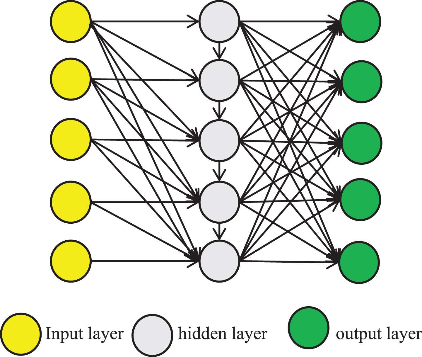
RNN deep learning algorithm framework.

Neuroimaging is a non-invasive technique used to acquire images of the brain, eliminating the need for surgical procedures, incisions, or direct internal contact. Due to its ability to visualize both the structure and function of the brain without causing harm, neuroimaging has emerged as a potent diagnostic tool in both research and clinical medicine [7]. As the central organ of the human central nervous system, the brain resides within and is safeguarded by the cranial vault. While sharing structural similarities with other mammals’ brains, it distinguishes itself through an extensively developed cortex. Enveloping most of this intricate organ, the human cerebral cortex comprises a substantial layer of neural tissue. The brain is further divided into interconnected right and left hemispheres via trabeculae and septa. The surface of the cerebral hemispheres is covered with sulci, and the slender part between the sulci is called the gyri. The depth and curvature of the sulci vary from individual to individual [8]. A schematic diagram of the longitudinal section of the brain is shown in Fig. 2, in which some major structures of the brain are marked in detail, including the cerebrum, cerebellum, brainstem, cerebral cortex, etc.

Fig. 2

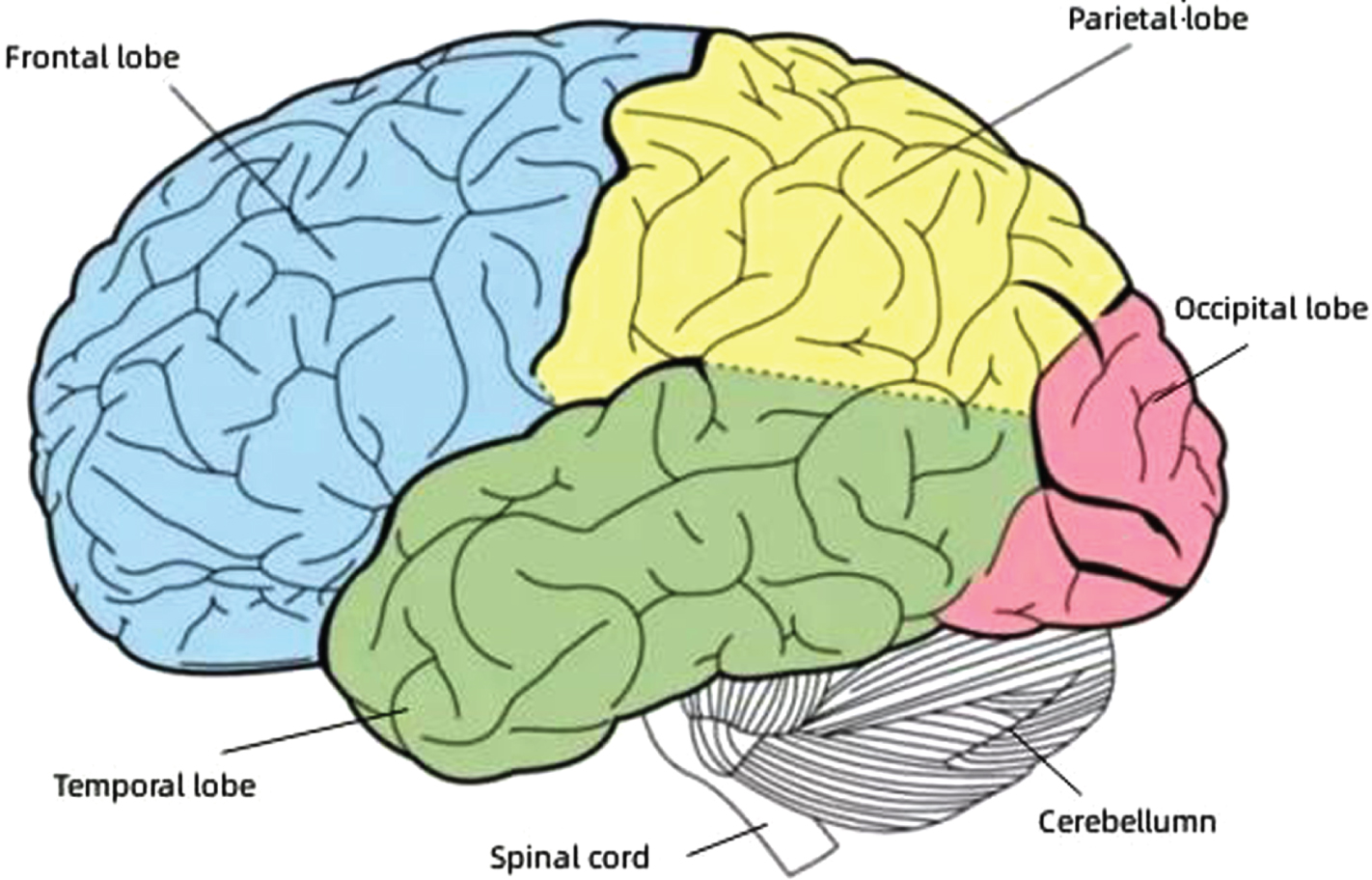
Diagram of major brain structures.

3 Application of feature extraction based on stacked auto-encoder network in the diagnosis of brain diseases

Studies have shown that Alzheimer’s disease (AD) and Mild Cognitive Impairment (MCI) are increasingly harmful to human health, but there is no effective treatment for AD/MCI at present. So in the clinic, the early diagnosis of AD/MCIMCI and prediction is particularly important, especially in the aging of the population today, even cause a small delay to the onset of AD and intervention, can also be a great help to health for all [9]. Therefore, with the help of the latest neuroimaging technology and network learning methods to assist diagnosis has become a new research field.

In the field of AD/MCI classification, many researchers have studied it from various aspects such as classifier training and multimodal image fusion, trying to improve the accuracy of AD/MCI classification. However, a significant limitation of the previous research lies in our exclusive consideration of simple low-level features for classification purposes. Therefore, with regards to feature extraction, this chapter assumes the existence of hidden or potential high-level feature information within these low-level features [10]. The incorporation of such latent feature information at higher development of more robust AD/MCI diagnostic and predictive models. To extract these high-level latent features effectively, we introduce a stacked autoencoder network in this section.

3.1 Sparse auto-encoder model

Combination with the characteristics of automatic encoder mining potential structure information, this paper adopts steam automatic encoder model, by minimizing the input signal and the reconstruction of the hidden layer stimulation output error to study said potential, compression of the input signal. Let D_H and D_I denote the number of units in the hidden layer and input layer in the neural network, respectively. Given a training sample of a set of N objects $X = {x_{i} \in R^{D_{I}}}_{i = 1}^{N}$ , its mapping is through a linear mapping and a nonlinear activation function $y_{i} = f (W_{1} x_{i} + b_{1})$ (1)

Where W₁ is the coding weight coefficient matrix and b₁ is the bias vector. For the activation function, in this paper

In this paper, we consider the unified use of the logical sigmoid function $f (a) = 1 / (1 + exp (1 - a))$ (2)

Logic sigmoid function is most widely used pattern recognition and machine learning field activation function [11]. From the viewpoint of learning and training, our purpose is to adjust the training parameters to minimize the error between input signal x_i and output signal z_i reconstruction. In this paper, we assume $Z_{i} = {z_{i}}_{i = 1}^{N}$ , To introduce sparse sex, use Kullback Leibler-to describe the average of the hidden layer neurons incentive intensity and the differences between the target average incentive intensity, the average excitation intensity of the first j a hidden layer neurons and target average incentive intensity is Bernoulli random variables. So the objective function can be described as: $l (X, X) + γ \sum_{j = 1}^{D_{H}} K L (ρ | | {\hat{ρ}}_{j})$ (3)

ρ is the labeled average excitation intensity and ${\hat{ρ}}_{j}$ is the average excitation intensity of the neurons in the hidden layer.

3.2 Feature extraction based on stacked auto-encoder network

Inspired by the great help of deep learning hierarchical architecture for improving high-level nonlinear and complex pattern features, this paper uses Stacked Auto-Encoder (SAE) to represent and extract features from neuroimaging and biological data. In this model, the auto-encoder is regarded as one component, and then they are stacked and connected sequentially [12]. The output of the lower hidden layer is used as the input of the higher input layer. The specific structure is shown in Fig. 3 below.

Fig. 3

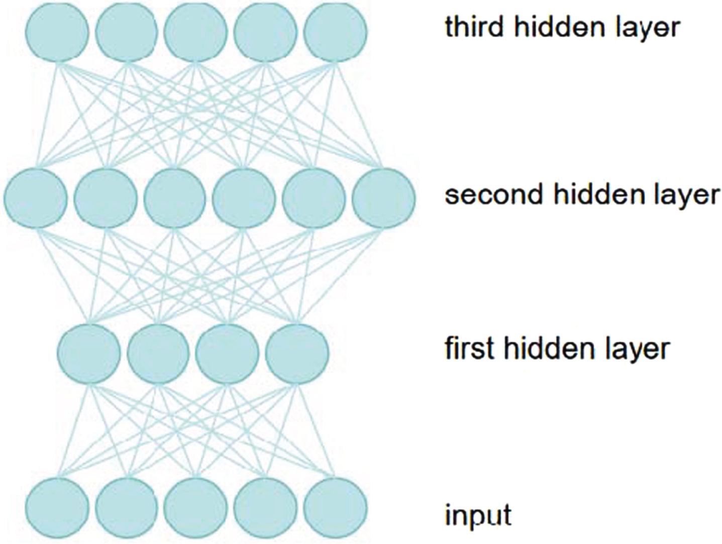
Three-layer structure stacked auto-encoder.

As can be seen from the Fig. 3, the number of input layer neurons and the dimensions of the input feature vectors are equal, an important characteristics of deep learning is characteristic of potential said can be obtained directly from the original data in the training [13]. Using its representable, self-learning nature, we can extract low-level features directly from neuro-images. For the training of the weight coefficient matrix and bias coefficient matrix parameters of our stacked auto-encoder model, the most direct method is to use the backpropagation algorithm and then update the parameters based on gradient optimization. It is equivalent to treating the stacked auto-encoder model as a traditional multi-layer artificial neural network, and the specific algorithm flow is as follows:

Input: Input feature vector set $X = {x_{i}}_{i = 1}^{N} \in R^{D_{I}}$ , stack auto-encoder layer number n_l

Output: weight coefficient matrix W_i, bias coefficient matrix b_i

Assign random initial values to weight coefficient matrix W_i and bias coefficient matrix b_i;

Some of them were randomly selected from the training samples as input data.

The output of the model was calculated according to the initial weight coefficient matrix and bias coefficient matrix.

The error between output and input and its partial derivatives for each neuron were calculated.

The weight coefficient and bias coefficient of the model were adjusted one by one according to the partial derivative value of error to each neuron.

After the reverse adjustment, whether the error met the requirements was judged, if so, the calculation was stopped. If not, step 5 will be re-executed.

Considering that the BP algorithm of the deep learning network is very sensitive to the initial value, the random initial weight coefficient matrix and bias coefficient matrix will lead to the inconsistent results of each training of the deep learning network, and the results will not reach the global optimal solution [14]. In this paper, according to the nature of the stacked auto-encoder model belongs to unsupervised learning, a supervised learning step is introduced, and the whole training and learning process is divided into pre-training and fine-tuning. It overcomes the problem that the derivation of deep neural network by BP algorithm is easy to fall into the local optimal solution.

3.3 Pre-training-fine-tuning two-step algorithm

The core of the pretraining-fine-tuning two-step algorithm is to train the weight coefficient and bias coefficient matrix of only one layer at a time, so that the operation can maximize the lower bound of the whole deep network [15]. The specific operation steps of the pretraining-fine-tuning algorithm are as follows: suppose that it is required to solve the bias coefficient matrix of the weight coefficient matrix of a two-layer stacked autoencoder. Input layer, the first and second hidden layer neurons number of hidden layers respectively for n1, n2, and n3.Coefficient of the connection between the input layer and the hidden layer parameters with W1, b1, said the connection between the first and second hidden layers of hidden layers on the coefficient parameters with W2, b2 said. Since the integrity of the encoder network stack type architecture as shown in Fig. 4.

Fig. 4

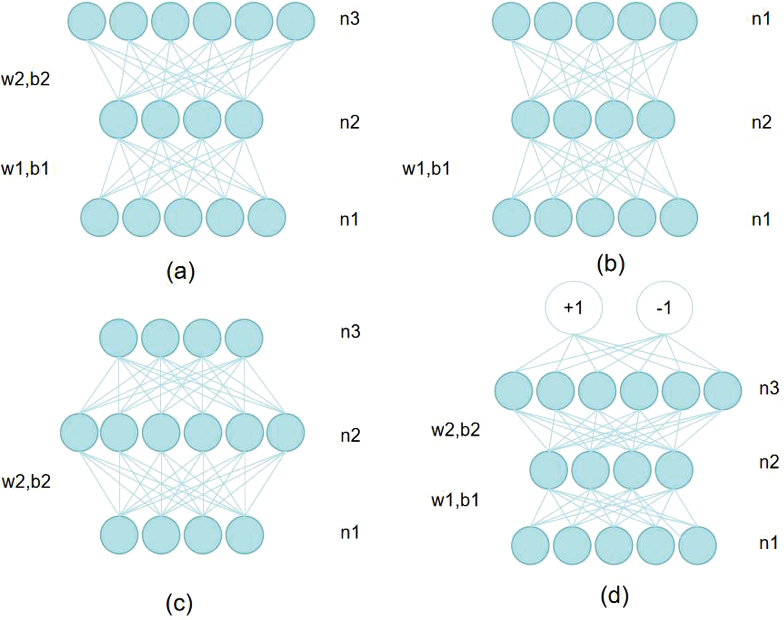
Pretraining-fine-tuning two-step algorithm flow.

From this figure, it can be seen that the pretraining-fine-tuning algorithm of the stacked auto-encoder is as follows:

Input: Training feature sample: X ∈ R^D₁×N, training sample label: L ∈ R^N, sparsity parameter: γ, target average activation intensity: ρ.

Output: weight coefficient matrix ${W_{l}^{h}}_{h = 1}^{H + 1}$ , bias coefficient matrix ${b_{l}^{h}}_{h = 1}^{H + 1}$ , where H represents the number of hidden layers.

Step 1: Pre-train the hidden layers

Initialize: Y₀ = X, for each hidden layer h∈ { 1, . . . , H }, the coefficient parameter ${W_{l}^{h}, b_{l}^{h}}$ is calculated, and the output $Y_{h} = f (W_{l}^{h} Y_{h - 1} + b_{l}^{h})$ is calculated based on this.

Step 2: Fine-tune the entire neural network

Initialize ${{\hat{W}}_{l}^{h} = W_{l}^{h}, \hat{b} l_{h} = b_{l}^{h}}_{h = 1}^{H}$ , ${{\hat{W}}_{l}^{H + 1}, {\hat{b}}_{l}^{H + 1}}$ take random values, and implement the backpropagation algorithm with the gradient descent technique.

3.3 Support vector machine classifier

To evaluate the efficacy of features extracted by the stacked sparse auto-encoder network, a classifier is employed to categorize data samples and classification accuracy is utilized to assess feature quality [16]. Support vector machine (SVM) was implemented for sample classification. Considering that what needs to be solved is the AD/MCI binary classification problem, only the binary support vector machine is considered below. C-SVC model is a more common binary support vector machine model, and the basic steps of its classification are as follows:

Let the training set be known $T = {(x_{1}, y_{1}), . . ., (x_{1}, y_{1})} \in (X \times Y)^{l}$ (4) Where,; x_i ∈ X = Rⁿ, y_i ∈ Y = { 1, - 1 } (i = 1, 2, . . . , l) x_i Is the eigenvector.

Select the appropriate kernel function K (x, x′) and the appropriate parameter C, construct and solve the optimization problem:

$min_{a} \frac{1}{2} \sum_{i = 1}^{j} \sum_{j = 1}^{l} y_{i} y_{j} a_{i} a_{j} K (x_{i}, x_{j}) - \sum_{j = 1}^{l} a_{j}$ (5) After calculation, the optimal solution is obtained as follows. a = (a₁, . . . , a₁) ^T

A positive component of is selected a = (a₁, . . . , a₁) ^T, and the threshold is calculated based on this: $b = y_{i} - \sum_{i = 1}^{l} y_{i} a_{i} K (x_{i} - x_{j})$ (6)

Construct the decision function: $f (x) = sgn (\sum_{i = 1}^{l} a_{i} y_{i} K (x, x_{i}) + b)$ (7)

The SVM classifier designed in this paper can realize a series of models such as binary classification support vector machine, multi-classification support vector machine, and linear separable vector machine by setting different parameters to solve regression and classification problems.

4 Experimental analysis

4.1 Experimental design

In order to verify the effectiveness of the feature extraction based on the stacked auto-encoder network constructed in this paper, this chapter takes typical brain disease features as an example to conduct experimental analysis to verify whether the features extracted by the stacked auto-encoder network constructed in this paper are more conducive to brain disease classification tasks. In order to ensure the coverage of the experimental data, 129 normal subjects, 98 AD patients, 136 MCI non-conversion patients and 67 MCI conversion patients were selected in this paper. The experiment was divided into four control groups. In the first experiments, the two cohorts consisted of patients with mild cognitive impairment (MCI) who converted to Alzheimer’s disease (AD) and patients with MCI who did not convert. The second set of control experiments, the two cohorts included AD patients and healthy individuals [17]. In the third group of control experiments, the two types of subjects were MCI patients (including MCI patients and non-MCI patients) and normal subjects. In the fourth control experiment, two types of subjects were AD patients and MCI patients (including conversion and non-conversion patients). On this basis, a set of comprehensive experiments were carried out, taking MCI patients and MCI non-converted patients as experimental subjects, combining the two steps of feature extraction based on stacked autoencoder to classify, calculating the classification accuracy and evaluating the performance of the proposed stacked auto-encoder in the feature extraction of the new classifier. The whole experimental process is as follows:

According to the idea of k-fold cross test, the whole dataset was divided into 10 parts, of which 9 parts were used as the training set and 1 part as the test set. Ten groups of training sets and 10 groups of corresponding test sets were obtained by cyclic operation 10 times.

The training set was used to learn a stacked auto-encoder model, and the parameters of the stacked auto-encoder model were adjusted by the pre-training-fine-tuning two-step algorithm. The label information of the training samples in the supervised learning was used to make the model reach the optimal solution.

The trained stacked auto-encoder model was used to extract features from the training set and the test set, respectively.

The primary and SAE features of the same training set were used to train the corresponding SVM classifier, and the primary and SAE features of the same test set were used for classification, respectively [18]. The classification accuracy, sensitivity and specificity were obtained and compared. The experimental flow chart is shown in Fig. 5 below.

Fig. 5

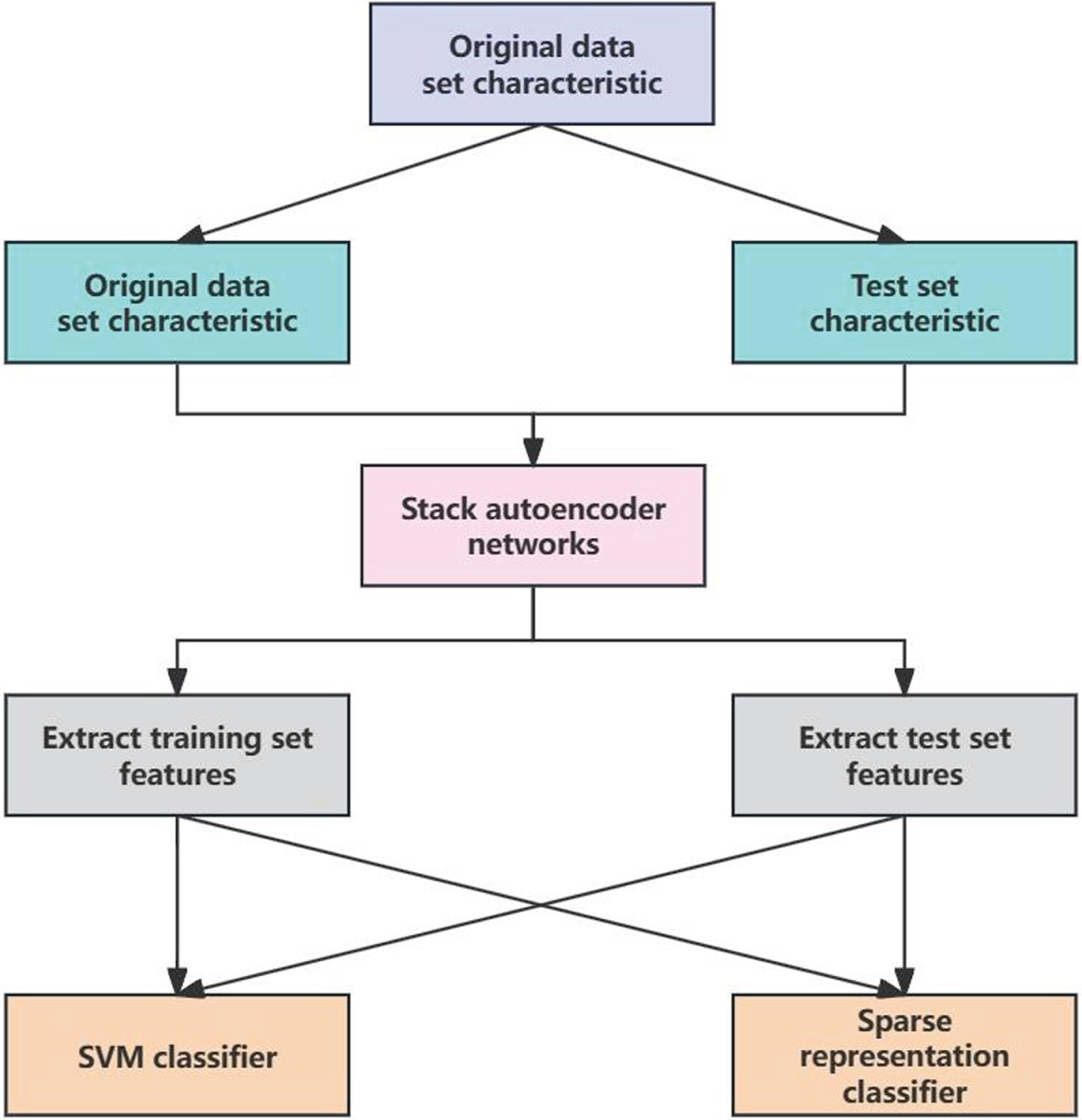
Experimental flow chart.

4.2 Analysis of experimental results

4.2.1 The first set of experiments

The experimental object is MCI-C and MC-NC. First, with the optimal parameters of the neural network training samples to determine stack, with the method of positive grid search, in turn, determine the three layers of hidden layer neurons number is 182105 and 10, respectively. Thus, for this set of experiments, the configuration of neurons in the stacked auto-encoder model was 93-182-105-10-93. The relationship between changes in neuron count within these hidden layers and classification accuracy is depicted in Figs. 6, 7, and 8.

Fig. 6

The relationship between the classification accuracy of the first hidden layer and the number of neurons.

Fig. 7

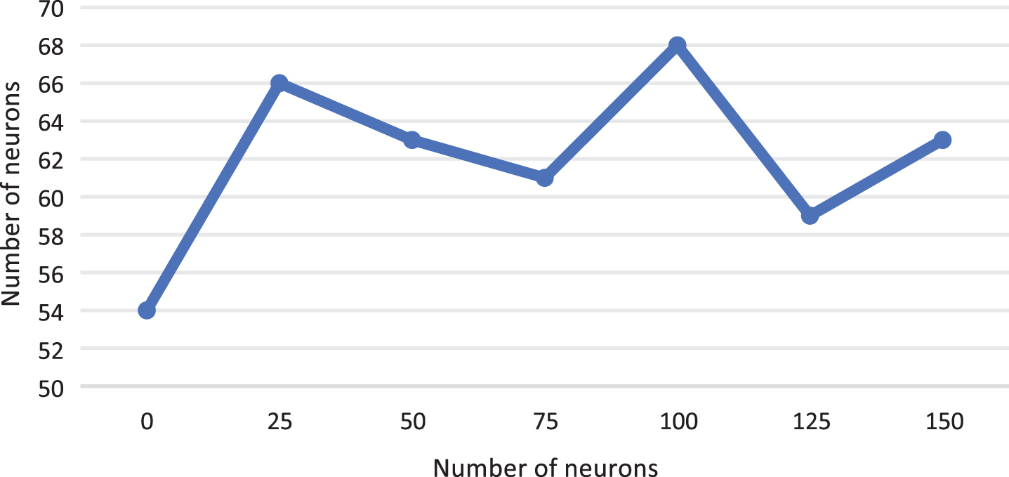
The relationship between the classification accuracy of the second hidden layer and the number of neurons.

Fig. 8

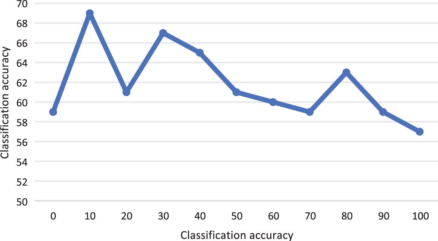
The relationship between the classification accuracy of the third hidden layer and the number of neurons.

After stacked auto-encoder network is obtained, the features of the original data samples can be extracted using the coefficient matrix. According to the number of neurons in the third hidden layer is 10, we know that the newly extracted feature is a 10-dimensional feature vector. This study includes the 93-dimensional primary extracted features (introduced as input) and the 10-dimensional SAE extracted features into the same SVM classifier. The classification accuracy, sensitivity and specificity results are shown in Table 1.

Table 1

Classification accuracy corresponding to different feature vectors of MCI-C vs MCI-NC

Feature categories	Primary extraction features	SAE extract features	Shallow layer extraction features
Classifier parameters	-s 0 –t 2 –c 1 –g 2. 3
Network structure	–	93-182-3 105-10-9	The 93-10-9 3
Accuracy Rate	65.3%	70.3%	60.3%
Sensitivity	44.9%	60.4%	40.4%
Specificity	79.6%	77.2%	74.5%

As can be seen from the data in the table, the classification accuracy of the features extracted by the simple shallow auto-encoder is not only lower than that of the features extracted by the stacked auto-encoder, but also lower than that of the original features. This is because the features extracted by the shallow auto-encoder only compress their dimension on the basis of retaining the original information to the greatest extent, which will inevitably lose part of the information that is conducive to classification, resulting in the decline of the classification accuracy.

4.2.2 The second set of experiments

The study involved patients with Alzheimer’s disease (AD) and individuals without the condition, serving as normal subjects. Initially, the training samples were utilized to determine the optimal parameters for the stacked neural network [19]. Through a forward grid search approach, the number of neurons in each of the three hidden layers was determined. Consequently, the structure of the stacked auto-encoder model was established as 93-48-148-33-93. By considering the neuron count in the third hidden layer, it was possible to ascertain that new features extracted by this stacked auto-encoder network would possess a dimensionality of 33. The specific experimental results are presented in Table 2 below.

Table 2
Classification accuracy corresponding to different feature vectors of AD vs NORMAL

Feature categories Primary extraction features SAE extract features Shallow layer extraction features

Classifier parameters -s 0 –t 2 –c 1 –g 1

Network structure – 93-48-148-33-93 93-31-93

Accuracy Rate 86.2% 87.6% 83.2%

Sensitivity 85.9% 84.9% 77.8%

Specificity 86.5% 90.0% 87.8%

Feature categories	Primary extraction features	SAE extract features	Shallow layer extraction features
Classifier parameters	-s 0 –t 2 –c 1 –g 1
Network structure	–	93-48-148-33-93	93-31-93
Accuracy Rate	86.2%	87.6%	83.2%
Sensitivity	85.9%	84.9%	77.8%
Specificity	86.5%	90.0%	87.8%

As can be seen from the data in the table, the classification accuracy of the feature vector extracted by SAE was slightly higher than that of the primary extraction, which increased from 86.2% to 87.6%, and the sensitivity and specificity changed from 85.9% and 86.5% to 84.9% and 90.0%, respectively. Similarly, we constructed a shallow auto-encoder with the structure of 93-33-93 to verify the effectiveness of the deep learning network. It can be seen that the classification accuracy of the features extracted by the shallow auto-encoder is only 83.2%.

4.2.3 The third set of experiments

The participants in this study consisted of individuals with mild impairment (including both those who converted to dementia and not) as well as healthy controls. Initially, the optimal parameters for the neural network were determined using the training samples. The forward grid search method was employed to calculate the number of neurons in each of the three hidden layers, resulting in 215, 207, and 61 neurons respectively. Thus, the network structure was defined as 93-215-207-61-93. Similarly, it was determined that the dimensionality of the newly extracted features would be 61. The specific experimental results are presented in Table 3 below.

Table 3
Classification accuracy corresponding to different feature vectors of MCI vs NORMAL

Feature categories Primary extraction features SAE extract features Shallow layer extraction features

Parameters of classifier -s 0 -T 2 -C 1 -G 2.3

Network structure – 93-215-207-61-93 93-62-93

Accuracy Rate 65.5% 70.5% 65.4%

Sensitivity 77.7% 77.8% 75.2%

Specificity 46.9% 49.1% 48.4%

Feature categories	Primary extraction features	SAE extract features	Shallow layer extraction features
Parameters of classifier	-s 0 -T 2 -C 1 -G 2.3
Network structure	–	93-215-207-61-93	93-62-93
Accuracy Rate	65.5%	70.5%	65.4%
Sensitivity	77.7%	77.8%	75.2%
Specificity	46.9%	49.1%	48.4%

As can be seen from the data in the table, the classification accuracy, sensitivity and specificity of the SAE extracted features are higher than those of the primary extracted features [20]. This shows that the stacked auto-encoder model we trained can well extract the potential high-level feature information from the original features, and these features are conducive to our classification task, that is to say, these features have a certain degree of discrimination.

4.2.4 The fourth set of experiments

The experimental object is patients with MCI and AD patients. In the first step, the optimal parameters of the neural network are determined using the positive grid search method in order to define the number of hidden neurons in each layer. Then, the number of hidden layer neurons obtained 171, 49, and 22. The experimental results are shown in Table 4 below.

Table 4
Classification accuracy corresponding to different feature vectors of MCI vs AD

Feature categories Primary extraction features SAE extraction features Shallow layer extraction features

Classifier parameters -s 0 -T 2 -C 1 -G 2.3

Network structure – 93-171-49-22-93 93-22-93

Rate of accuracy 69.2% 74.9% 70.8%

Sensitivity 44.2% 48.9% 51.1%

Specificity 72.3% 83.0% 71.2%

Feature categories	Primary extraction features	SAE extraction features	Shallow layer extraction features
Classifier parameters	-s 0 -T 2 -C 1 -G 2.3
Network structure	–	93-171-49-22-93	93-22-93
Rate of accuracy	69.2%	74.9%	70.8%
Sensitivity	44.2%	48.9%	51.1%
Specificity	72.3%	83.0%	71.2%

According to the data in the table, the feature extraction work of this group was also done well, and the classification accuracy of the feature vector extracted by SAE increased by 5 percentage points.

4.2.5 Comprehensive experiments

To investigate the effect of feature extraction on the data of multiple time points, we trained the corresponding feature extraction network with the data of five time points. The experimental objects were MCI-C and MCI-NC patients, and the solution for the data object without multiple time points was to replace the data of the benchmark time point. The experimental results are shown in Table 5 below.

Table 5
Comparison of feature extraction accuracy of MCI-C vs MCI-NC at multiple time points

Point of time Stack auto-encoder network parameters Primary extraction special diagnosis SAE extraction features

1 93-182-3 105-10-9 65.4% 70.4%

2 93-89-3 100-10-9 68.2% 70.6%

3 93-173-3 103-10-9 69.1% 70.4%

4 93-89-3 152-10-9 66.8% 70.8%

5 93-148-100-60-93 67.6% 71.2%

Average – 67.4% 70.6%

Point of time	Stack auto-encoder network parameters	Primary extraction special diagnosis	SAE extraction features
1	93-182-3 105-10-9	65.4%	70.4%
2	93-89-3 100-10-9	68.2%	70.6%
3	93-173-3 103-10-9	69.1%	70.4%
4	93-89-3 152-10-9	66.8%	70.8%
5	93-148-100-60-93	67.6%	71.2%
Average	–	67.4%	70.6%

In addition, also by ROC curve drawing (ReceiverOperatingCharacteris - ticCurve) to calculate the area under the curve to evaluate the SAE to extract the features, the primary extraction and shallow to extract features of performance. The receiver operation characteristic curve is obtained by tracing the true positive rate as the vertical axis and the false positive rate as the horizontal axis under different threshold conditions. The receiver manipulates the feature curve as a tool to help us select an optimal model and discard the remaining models that do not meet the optimal criteria without relying on the threshold and sample class distribution. The closer the receiver operation characteristic curve is to the vertical axis, that is, the area under the curve is close to 1, indicating the better performance of the classifier. The specific results are shown in Fig. 9 below.

Fig. 9

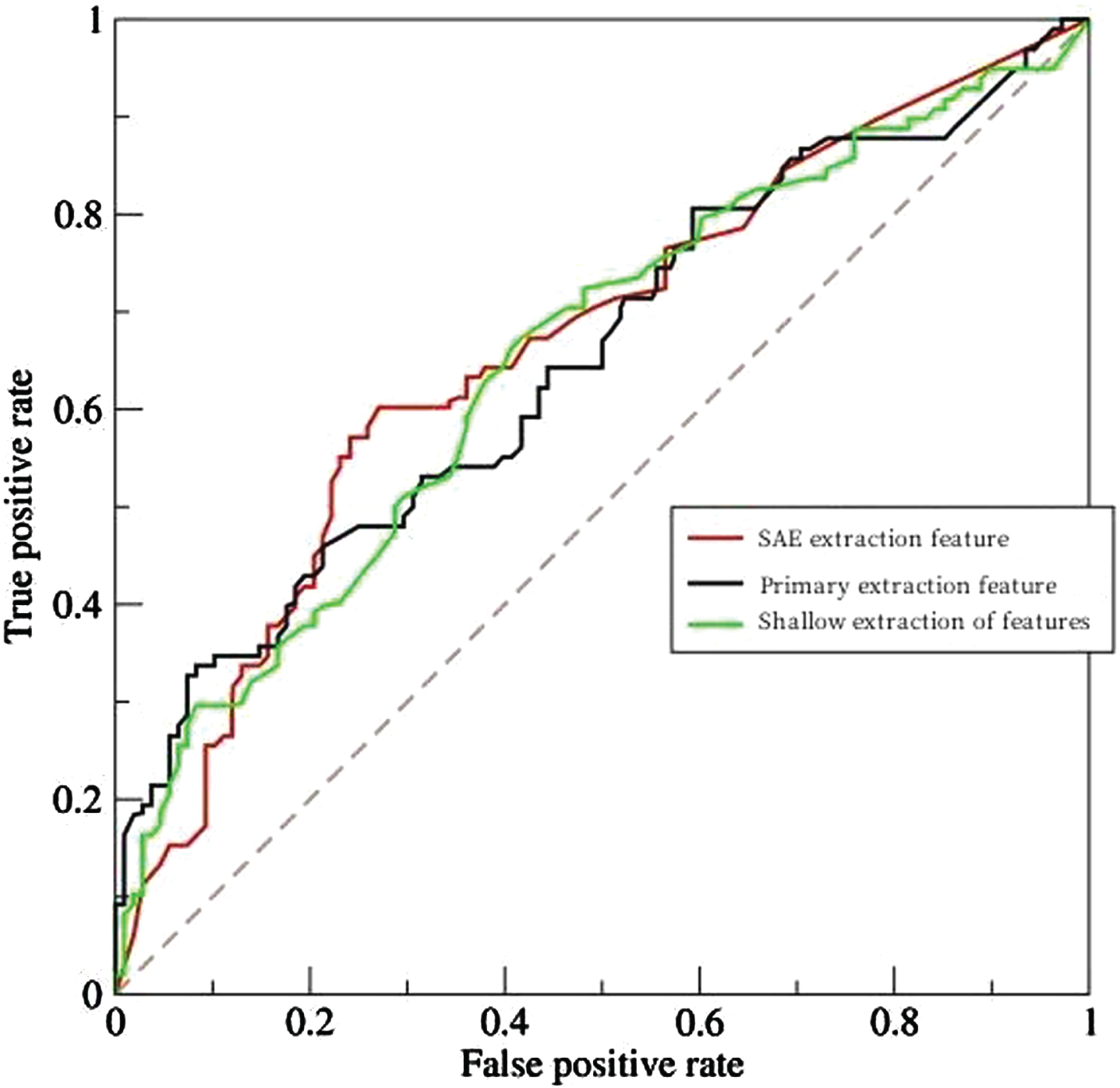
Receiver operation characteristic curves of different methods.

It can be seen from the data in Table 5, the accuracy of features extracted by the stacked autoencoder network is 3.2% higher than that of the primary extraction. Combined with the ROC curve, it is sufficient to prove that the operation of feature extraction by using the stacked autoencoder in the deep learning network for the original data samples is completely feasible and effective. Abstract and extracted features perform better when applied to classification tasks.

5 Conclusion

To sum up, as the most common brain diseases are cerebrovascular diseases and brain tumors, which are of great harm to human health, an accurate diagnosis system can provide help for the treatment of brain diseases. In this paper, the feature diagnosis of brain diseases such as AD and MCI is studied based on the neuroimage technology of deep learning algorithm, and a feature extraction method based on stacked autoencoder network is designed. The experiment verifies that the method has better accuracy and better classification performance than the traditional primary feature extraction. However, on the other hand, this study mainly focuses on the diagnosis of AD and MCI brain diseases, so whether the feature extraction method based on the stacked autoencoder network can be applied to other types of brain diseases needs to be further verified. In the future research work, the author will continue to improve the feature extraction method of the stacked autoencoder network. Finally, a learning algorithm covering multiple types of brain diseases is established.

References

Babin

, Pizurica

, Bellens

, et al. Generalized pixel profiling and comparative segmentation with application to arteriovenous malformation segmentation[J], Medical Image Analysis 16(5) (2012), 991–1002.

Nyoman Abiwinanda

M.H.S.T.

, A.T.R.M. Astri Handayani, Brain Tumor Classification Using Convolutional Neural Network[J]. 2018.

Talo

, Baloglu

U.B.

, Yıldırım

Ö.

, et al. Application of deep transfer learning forautomated brain abnormality classification using MR images[J], Cognitive Systems Research 54 (2019), 176–188.

Weina

and Feng

, Progress in neuroimaging research of episodic memory dysfunction in AD spectrum patients mediated by default network subsystem [J], Journal of Chongqing Medical University 46(11) (2021), 1395–1398.

Ali

and Rehman

J.A.

, Privacy Preserved Brain Disorder Diagnosis Using Federated Learning, 47(2) (2023), 2187–2200.

Tammam

, Veit

, Dorothee

, et al. Mini review: Current status and perspective of S100B protein as a biomarker in daily clinical practice for diagnosis and prognosticating of clinical outcome in patients with neurological diseases with focus on acute brain injury, BMC Neuroscience 24(1) (2023), 38–38.

Deep

A.A.

, Singh

V.S.

, Prasun

, et al. A systematic review on machine learning and deep learning techniques in the effective diagnosis of Alzheimer’s disease, Brain Informatics 10(1) (2023), 17–17.

Anna

, Alan

, Barry

, et al. The Role of Magnetic Resonance Imaging in Diagnosing Fetal Brain Pathologies, Radiologic Technology 94(6) (2023), 430–434.

Martin Nicholas

, Hiroaki

, Minji

, et al. Brain Bank Questionnaire Helps in Differential Diagnosis of Movement Disorders: An Autopsy Study of 150 Patients, Movement Disorders Clinical Practice 10(7) (2023), 1131–1135.

10.

Cristina

, Luigi

M.A.

, Elias

, et al. Brain-Biomarker Changes in Body Fluids of Patients with Parkinson’s Disease, International Journal of Molecular Sciences 24(13) 2023.

11.

Shinobu

and Ryota

, Towards Improved Clinical Diagnosis of Argyrophilic Grain Disease Using Brain Imaging, Journal of Alzheimer’s Disease: JAD 93(1) (2023), 389–392.

12.

SeyedAli

S.Z.

, Elham

, Mahboobe

, et al. An Approach toward Artificial Intelligence Alzheimer’s Disease Diagnosis Using Brain Signals, Diagnostics 13(3) (2023), 477–477.

13.

Besma

, Ahmed

B.H.

, Nidhal

, et al. Contribution of Brain Regions Asymmetry Scores Combined with Random Forest Classifier in the Diagnosis of Alzheimer’s Disease in His Earlier Stage, Journal of Medical and Biological Engineering 43(1) (2023), 74–82.

14.

ZhiGuo

, Jie

, Jun

, et al. Nucleic acid drug vectors for diagnosis and treatment of brain diseases, Signal Transduction and Targeted Therapy 8(1) (2023), 39–39.

15.

Xin

, Usman

R.M.

, Gongbo

, et al. Efficient Training on Alzheimer’s Disease Diagnosis with Learnable Weighted Pooling for 3D PET Brain Image Classification, Electronics 12(2) (2023), 467–467.

16.

Sandroff Brian

, Rafizadeh Caroline

, Motl Robert

, et al. Neuroimaging Technology in Exercise Neurorehabilitation Research in Persons with MS: A Scoping Review, Sensors 23(9), 2023.

17.

Vedula

R.R.

and Kolathu

R.M.

, Birth and Growth of Neuroimaging and Vascular Intervention at Sree Chitra Tirunal Institute for Medical Sciences & Technology, Thiruvananthapuram—Part I, Journal of Clinical Interventional Radiology ISVIR 6(1) (2022), 28–36.

18.

Vedula

R.R.

and Kolathu

R.M.

, Birth and Growth of Neuroimaging and Vascular Intervention at Sree Chitra Tirunal Institute for Medical Sciences & Technology, Thiruvananthapuram—Part II, Journal of Clinical Interventional Radiology ISVIR 6(1) (2022), 37–42.

19.

Janssen Tieme

W.P.

, Grammer Jennie

, Bleichner Martin

, et al. Opportunities and Limitations of Mobile Neuroimaging Technologies in Educational Neuroscience, Mind, Brain, and Education 15(4) (2021), 354–370.

20.

Zeng

H.-M.

, Han

H.-B.

, Zhang

Q.-F.

, et al. Application of modern neuroimaging technology in the diagnosis and study of Alzheimer’s disease, Neural Regeneration Research 16(1) (2021), 73–79.

21.

Choi

, Kim

Y.K.

, Yoon

E.J.

, et al. Cognitive signature of brain FDG PET based on deep learning: domain transfer from Alzheimer’s disease to Parkinson’s disease, Eur J Nucl Med Mol Imaging 47 (2020), 403–412. https://doi.org/10.1007/s00259-019-04538-7

22.

, Zhao

, Huang

, et al. Functional Brain Network Classification for Alzheimer’s Disease Detection with Deep Features and Extreme Learning Machine, Cogn Comput 12 (2020), 513–527. https://doi.org/10.1007/s12559-019-09688-2

23.

Ahmed

H.M.

, Elsharkawy

Z.F.

and Elkorany

A.S.

, Alzheimer disease diagnosis for magnetic resonance brain images using deep learning neural networks, Multimed Tools Appl 82 (2023), 17963–17977. https://doi.org/10.1007/s11042-022-14203-1

24.

Zhao

, Li Huajin

, et al. Presenting a novel approach based on deep learning neural network and using brain images to diagnose Alzheimer’s disease, Proc.Indian Natl. Sci. Acad (2023). https://doi.org/10.1007/s43538-023-00198-2.

25.

Ryoo

H.G.

, Choi

, Shi

, et al. Distinct subtypes of spatial brain metabolism patterns in Alzheimer’s disease identified by deep learning-based FDG PET clusters, Eur J Nucl Med Mol Imaging (2023). https://doi.org/10.1007/s00259-023-06440-

26.

Roopa

Y.M.

, Reddy

B.B.

, Babu

M.R.

, et al. Teaching learning-based brain storm optimization tuned Deep-CNN for Alzheimer’s disease classification, Multimed Tools Appl 82 (2023), 33333–33356. https://doi.org/10.1007/s11042-023-14815-1

27.

Tinauer

, Heber

, Pirpamer

, et al. Interpretable brain disease classification and relevance-guided deep learning, Sci Rep 12 (2022), 20254. https://doi.org/10.1038/s41598-022-24541-7

28.

Balnarsaiah

, Nayak

B.A.

, Sujeetha

G.S.

, et al. Parkinson’s disease detection using modified ResNeXt deep learning model from brain MRI images, Soft Comput 27 (2023), 11905–11914. https://doi.org/10.1007/s00500-023-08535-9

29.

Kim

J.S.

, Han

J.W.

, Bae

J.B.

, et al. Deep learning-based diagnosis of Alzheimer’s disease using brain magnetic resonance images: an empirical study, Sci Rep 12 (2022), 18007. https://doi.org/10.1038/s41598-022-22917-3

30.

Etminani

, Soliman

, Davidsson

, et al. A 3D deep learning model to predict the diagnosis of dementia with Lewy bodies, Alzheimer’s disease, and mild cognitive impairment using brain 18F-FDG PET, Eur J Nucl Med Mol Imaging 49 (2022), 563–584. https://doi.org/10.1007/s00259-021-05483-0

31.

, Li

H.X.

, Chang

Z.K.

, et al. A practical Alzheimer’s disease classifier via brain imaging-based deep learning on 85,721 samples, J Big Data 9 (2022), 101. https://doi.org/10.1186/s40537-022-00650-y

32.

Goenka

and Tiwari

, Deep learning for Alzheimer prediction using brain biomarkers, Artif Intell Rev 54 (2021), 4827–4871. https://doi.org/10.1007/s10462-021-10016-0

33.

Oliveira

A.M.

, Coelho

, Carvalho

, et al. Machine learning for adaptive deep brain stimulation in Parkinson’s disease: Closing the loop, J Neurol 270 (2023), 5313–5326. https://doi.org/10.1007/s00415-023-11873-1