Prediction of PM 2.5 with a piecewise affine model considering spatial-temporal correlation

Abstract

Over the past several decades, several air pollution prevention measures have been developed in response to the growing concern over air pollution. Using models to anticipate air pollution accurately aids in the timely prevention and management of air pollution. However, the spatial-temporal air quality aspects were not properly taken into account during the prior model construction. In this study, the distance correlation coefficient (DC) between measurements made in various monitoring stations is used to identify appropriate correlated monitoring stations. To derive spatial-temporal correlations for modeling, the causality relationship between measurements made in various monitoring stations is analyzed using Transfer Entropy (TE). This work explores the process of identifying a piecewise affine (PWA) model using a larger dataset and suggests a unique hierarchical clustering-based identification technique with model structure selection. This work improves the BIRCH (Balanced Iterative Reducing and Clustering using Hierarchies) by introducing Kullback-Leibler (KL) Divergence as the dissimilarity between clusters for handling clusters with arbitrary shapes. The number of clusters is automatically determined using a cluster validity metric. The task is formulated as a sparse optimization problem, and the model structure is selected using parameter estimations. Beijing air quality data is used to demonstrate the method, and the results show that the proposed strategy may produce acceptable forecast performance.

Keywords

PWA model prediction of air pollutants spatial-temporal features hierarchical clustering-based identification

1 Introduction

As industrialization and urbanization pick up speed, a lot of harmful substances to human health are released into the atmosphere, including particulate pollutants like PM_2.5 and PM₁₀ and gaseous pollutants like SO₂, NO₂, O₃, and CO. This leads to several air pollution issues and an ecological environment crisis. Long-term, continuous haze pollution events are common in China’s Beijing-Tianjin-Hebei region, Yangtze River Delta, Pearl River Delta, and other economically developed areas. These events not only reduce atmospheric visibility but also raise the risk of respiratory illnesses and human mortality. Beijing is part of the Beijing-Tianjin-Hebei area, which is known for its regular haze and extensive media attention to air pollution. Regional air pollution and ozone pollution are becoming more noticeable, and the soot type of pollution has given way to compound type pollution in ambient air quality.

Because it contains more dangerous and poisonous chemicals, as well as microbes, atmospheric particle matter, is bad for human health. The component of atmospheric particulate matter that is most important is PM_2.5. PM_2.5 particles can remain in the atmosphere for a very long period because they are less susceptible to influence from various forms of atmospheric circulation and meteorological disturbances. They may be transferred across vast distances, which puts human health at greater risk. High PM_2.5 concentrations increase heart and lung disease incidence and death rates [1]. A brief exposure significantly increases the chance of dying from heart disease. According to Atkinson et al. (2014), there is a 1% average increase in deaths from all causes and a 0.8% increase in deaths from heart disease for every 10μg/m3 increase in transient PM_2.5 exposure worldwide. Long-term, chronic exposure to contaminated surroundings causes oxidative stress to cells and persistent inflammation [2].

Delicate particulate matter and other air pollutants have dramatically dropped in recent years as a result of China’s execution of air pollution prevention and control initiatives. Still, there are instances when the PM_2.5 concentration is higher than the allowable amount. Therefore, effective forecasting, management, and monitoring of air quality can minimize financial losses while promoting public health. If simple, accurate, and dependable models are available, then model-based analysis and decision methods may be developed to improve the development of air protection measures, including the restructuring of social activities. However, air pollution is a complex nonlinear dynamic process that is influenced by several factors, including geographical and meteorological circumstances. Given its complexity, robust, accurate, and straightforward air pollution modeling is still a distant objective. We then reframed the problem to look at the spatial-temporal evolution aspects of air quality, and our effort aims to address the following problems. First, we acknowledge the emergence of certain tendencies in meteorological elements. Multiple models are required to handle different weather patterns because different weather patterns result in different modes of air quality progression [3]. In addition, the link between stations is complex; air pollution is dispersed over a large region and may be affected by topography, natural events, meteorological phenomena, or other variables. In addition, the characteristics of air quality are produced sequentially and are a temporal series.

We propose a piecewise affine model to estimate air quality that takes meteorological and spatial-temporal characteristics into account to address the aforementioned problems. Regarding the temporal distribution of PM_2.5, it is seen that there is a high correlation between the current instant and a specific previous moment of monitoring stations. The temporal data of air pollutants is combined with auxiliary information, such as meteorological data, to further reflect the spatial-temporal correlation between the sites. The delayed timing values are then fed into the model to improve the depiction of the spatial-temporal link between the sites. To choose appropriate correlated monitoring stations, we first investigate the distance correlation coefficient (DC) between the measurements in various stations. Next, by calculating the Transfer Entropy (TE) between time series collected at various monitoring stations, the causality analysis is carried out. This yields the pertinent temporal and geographical properties, and based on the features collected, a unique hierarchical clustering algorithm is used to identify a PWA model. Recently, the BIRCH approach has gained a lot of attention for its effectiveness as a hierarchical agglomerative clustering technique. BIRCH was created to handle bigger datasets using a tree structure; it only needed to sift through the entire dataset once to achieve clustering [4]. However, according to [5], the method is insufficient for clusters with arbitrary forms or fluctuating volumes. Ren et al. proposed a novel hierarchical clustering method that has been employed in air quality forecasting to improve the regularity of the data [6]. This method extends a refinement phase to BIRCH, wherein clusters with the nearest distances are merged until the specified number of clusters is reached. This paper modified the method in [6] and employed the Kullback-Leibler (KL) Divergence to quantify cluster similarity. Unlike the Euclidean distance, the KL Divergence describes the distribution of data and is more adequate for clusters with variable volumes or arbitrary shapes. The Davies-Bouldin index (DBI), which calculates the dispersion of each cluster and the dissimilarity between two clusters, is automatically used to estimate the number of clusters. Furthermore, the proposed modeling approach forecasts Beijing’s air pollution. It should be mentioned that various model types may be included in the suggested technique, which is rather comprehensive.

The significant contributions of this work are:

To select appropriate correlated monitoring stations, this work uses the distance correlation coefficient (DC) between measurements in different stations. Then, to derive spatial-temporal correlations for modeling, the causality relationship between measurements in different monitoring stations is analyzed using Transfer Entropy (TE).

This study presents a modified version of BIRCH, which incorporates the KL Divergence to measure the cluster similarity. The Davies-Bouldin index (DBI) is automatically used to calculate the number of clusters.

The effectiveness of the suggested model is evaluated and the proposed PWA model is used to forecast PM_2.5 in Beijing. Experiments indicate that our model outperformed baseline models when comparing PWA models with baselines.

2 Related work

There are two main ways to create models of air pollution: data-driven or empirical models that are based on observations, and theoretical or deterministic models that are based on natural and artificial rules. Theoretical models describe the mechanics behind pollution emissions, dispersion, transport, diffusion, and removal using algebraic differential equations based on the physics and chemistry of the atmosphere. The structure of theoretical models is essentially determined by chemical formulae, as well as the laws of conservation of mass and energy. Typical physical models include Gaussian diffusion [7, 8], Community Multiscale Air Quality (CMAQ) [9 –11], the Comprehensive Air-quality Model with eXtension (CAMx) [12], and Weather Research and Forecasting (WRF) [13, 14].

Empirical models, on the other hand, are data-driven and use statistical and machine-learning techniques to identify patterns in observations that provide insights into the dynamics of pollutants. Although theoretical models offer a mechanical explanation, empirical models need substantial data sets to have sufficient prediction ability. When built, nevertheless, they can capture nonlinear motion that is overlooked by models that lack specific information. The resulting process model explains the interactions among complicated pollutant concentration data and captures the nonlinear dynamics of pollution. In general, data-driven models may be classified as either developing deep learning techniques or classic machine learning approaches. Conventional machine learning uses algorithmic and statistical techniques to find patterns, such as decision trees, clustering, and regression. Even though these methods are economical in terms of computing, they have trouble handling intricate and nonlinear processes. To get sufficient prediction performance, they need extensive preprocessing of the data and feature engineering. Classical machine learning models include the Autoregressive Integrated Moving Average (ARIMA) model [15], Multi-Linear Regression (MLR) model [16], Fuzzy Logic (FL) [17, 18], Takagi-Sugeno (TS) model [6], Adaptive Neuro-Fuzzy Inference System (ANFIS) [19 –24], Support Vector Machine (SVM) [15 , 25–27], Random Forest (RF) [28], Support Vector regression (SVR) [29], and Artificial Neural Network (ANN) model [30 –32] have all been widely used for air pollutant forecasting.

Deep learning algorithms use multilayer neural networks that learn a hierarchy of abstract ideas to find complex patterns in raw data. In fields where standard modeling approaches have failed, such as image processing, natural language translation, and medical diagnosis, deep learning has made significant strides possible. Deep learning can provide light on pollution dynamics that are too complex for traditional machine learning and unavailable to theory alone in environmental applications. Data and algorithms, when combined with physical knowledge, show promise for creating reliable environmental models that offer useful insights. However, there are still difficult issues with model complexity, data needs, and performance optimization when it comes to creating and implementing data-driven approaches for pollution modeling. In general, multidisciplinary cooperation is necessary for growth. In recent years, various network models have been proposed, like Convolutional Neural Network (CNN) [33], Graph Convolutional Neural network (GCN) [34], Recurrent Neural Network (RNN) [35 –37], Gated Recurrent Unit (GRU) [38 –40], Long Short-Term Memory (LSTM) [41 –44], Bidirectional Long Short-Term Memory (Bi-LSTM) [45, 46], and Convolutional Neural Network-Long Short-Term Memory (CNN-LSTM) [47, 48], and ResNet (Residual Neural Network) with CNN-LSTM [49].

Although theoretical models provide valuable insights into the mechanisms underlying pollutant diffusion, they are beset by several difficulties, such as the need for 1) substantial historical data, 2) dependable model parameters, and 3) substantial knowledge of environmental theories—demands that are time-consuming and require specialized expertise. In addition, uncertainties result from variations between model assumptions and actual conditions as well as from inaccurate, randomized parameter choices. In the end, these uncertainties compromise the model’s resilience and capacity to accurately depict shifts impacting the dynamics of pollution. The nonlinearity of the complex parameters influencing pollutant dynamics and the ease with which they transfer across circumstances are not adequately captured by theoretical models [47, 50]. As such, theoretical models frequently exhibit poor performance. Data-driven modeling, which typically performs better than theoretical techniques, has been prompted by these issues. Although data-driven methods have advantages such as resilience, nonlinear approximation, and self-learning, they are not without limitations. Because they identify basic patterns and exclude complicated correlations in large, high-dimensional data sets, traditional machine-learning algorithms are limited to using small datasets [50, 51]. Their applicability is restricted.

On the other hand, deep learning has made significant progress possible in challenging, data-intensive tasks that are outside the scope of standard machine learning models and theory. Deep learning is quite good at finding complex patterns in nonlinear, high-dimensional data. As such, deep learning models for pollutant concentration prediction often perform better than conventional methods [50]. Directly from raw data, deep neural networks extract hierarchical characteristics [52, 53]. Deep models do, however, confront significant limitations, including high computational complexity, restricted interpretability, and transferability [50, 51]. There is a need for models with simpler structures and lower computational efforts.

As a potent data-driven method frequently employed in complex system analysis, prediction, and simulation, piecewise affine (PWA) modeling has attracted a lot of attention [54 –56]. An affine sub-model represents each polyhedral area that PWA models divide the input space into. PWA models approximate nonlinear dynamics globally. An affine function describes the mapping locally from inputs to outputs within each area. PWA models offer accurate approximation with less complexity than purely nonlinear approaches by balancing local and global nonlinearity. PWA models provide practical advantages for modeling real-world processes when data and processing capacity are restricted because of this balance between performance and parsimony. To create integrated models that are reliable and precise enough to inform planning and policy, PWA modeling generally provides one possible link between theory and data-driven techniques. It is difficult to identify PWA models because it is needed to: 1) divide the input space into different parts; 2) estimate the borders of each partition; and 3) find the sub-model parameters for each region [57 –59]. According to [59, 60], coupling partition and parametrization issues make PWA model identification NP-hard [61]. There have been several PWA modeling approaches put out [54–56 , 62–64]. The use of clustering-based techniques, which separate data into homogenous groups, is growing in popularity. These techniques allow for increased generalizability, shorter training times, and similar training sets. Sub-model parameters may be computed sequentially or concurrently.

3 Problem statement

3.1 Study area

China’s capital city, Beijing, will be the subject of this investigation. Beijing, the political, economic, and cultural hub of China, is rapidly urbanizing and developing economically. Beijing, whose total area is 16 410 km2, is situated in the middle latitudes of 39°28 ^′ ∼ 41°02′ north and 115°25′∼ 117°30′ east. The Chaobai River and Yongding River alluvial great plains are located in the middle and south, while the Taihang Mountains and Yanshan Mountains are located in the west and north. The average annual temperature is 10 ∼ 12°C, January –7∼–4°C, July 25 ∼ 26 °C. The climate is characteristic of a mild temperate subhumid continental monsoon, with hot and wet summers and cold, dry winters. Rainfall totals are 600 mm on average each year. The brown zone is where the dirt is found. The Bohai Sea receives around 200 different rivers, both big and tiny. In Fig. 1, the research area is displayed.

Fig. 1

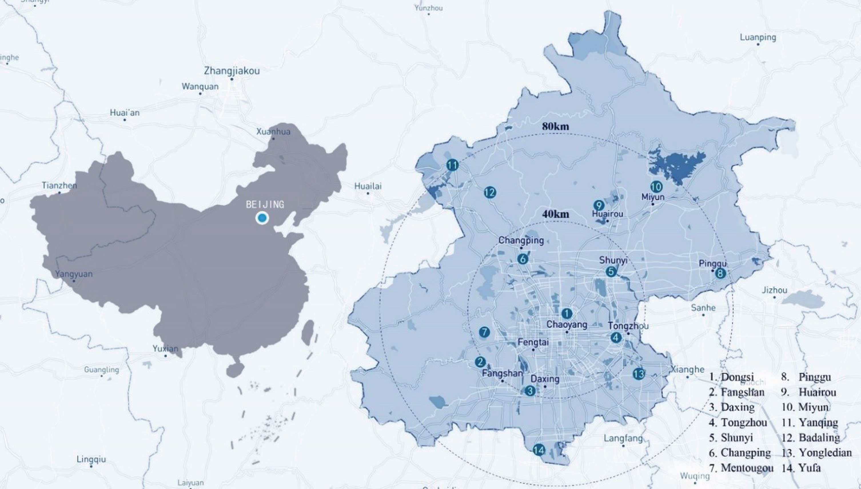
Study area with monitoring stations.

Beijing, one of the most prominent economic hubs in China, has a lot of elements affecting its atmosphere, including central heating, transportation, urbanization, and pollutant dispersion. Plans for air pollution prevention and management have even been put into place. Particulate Matter (PM), which is mostly released by vehicles, central heating, and industry, is the main source of air pollution in Beijing. The monthly average concentrations of PM_2.5 in Beijing are displayed in Fig. 2 (left), which highlights important monthly PM_2.5 features in Beijing. As seen in Fig. 2 (left), monthly average mass concentrations of PM_2.5 were at their highest in January 2017 (PM_2.5 = 110.95μg/m³) and at their lowest in May (PM_2.5 = 38.55μg/m³) and August (PM_2.5 = 38.63μg/m³). The monthly average PM2.5 observed in various monitoring sites for 2017 is displayed in Fig. 2 (right).

Fig. 2

Average monthly PM2.5 concentration in Beijing (left) and different stations (right) in 2017.

Beijing’s population is rapidly growing, and this is contributing to the city’s overall energy usage rising. Since coal has historically made up the majority of Beijing’s fuel mix, the city’s high concentration and variety of air pollutants, mostly soot and sulfur dioxide emissions from the direct burning of industrial and civic coal, are typical of the soot-type pollution. Wintertime is the worst season for direct coal-burning air pollution. Beijing’s cold, dry winters force heating to last for up to four months, which raises emissions of sulfur dioxide and soot dramatically.

When combined with ground dust, this typically results in a sharp reduction in visibility in metropolitan areas, particularly when it comes to urban air pollution. The most dangerous ones are those that are in commercial and industrial zones, have non-central heating, or have a lot of street manufacturers. Furthermore, the intensity of pollution sources’ emissions determines the level of air pollution, which is closely correlated with weather. The concentration and variation of air pollutants are mostly governed by atmospheric diffusion conditions when the emission intensity of a pollution source is largely constant.

The primary elements influencing the environment in which pollutants diffuse are wind and atmospheric stability. Beijing has strong, erratic winds from the north throughout the winter, which makes it easier for pollutants to diffuse, dilute, and travel around the city. As a result, if cold air arrives, the amount of pollutants in the atmosphere will rapidly drop and become much less than before. Nonetheless, the lower atmosphere becomes more stable as cold air becomes weaker and wind speed decreases. Pollutant diffusion is hampered by the dry, chilly air, bright, and less overcast weather, as well as by the presence of additional radiation inversion layers, particularly in the winter. The implementation of pollution prevention and control measures, like as traffic restrictions, coal burning regulation, and centralized management of point source and non-point source pollution, has improved Beijing’s air environment in recent years. However, Beijing’s air pollution situation has not fundamentally changed as a result of economic expansion. Beijing has a high degree of urbanization, which complicates the link between urbanization and environmental pollution and makes management and control more challenging. Air quality deteriorates as a result of population agglomeration, the building industry’s rapid growth, and a rise in motor vehicles brought on by urbanization. Urbanization will also result in industrial agglomeration, reduce emissions, and accomplish the scale impact of pollution control, all while reducing air pollution. The direction of the predominant wind throughout winter and summer has a considerable impact on the pollutants’ dispersion, dilution, and impacted area.

3.2 Available data

As mentioned before, factors affecting air quality include geography, climatic change, social and economic conditions, and pollution emissions. To anticipate future pollution, the previous variance in air pollutant emissions will be used as a reference. The primary factor influencing the change in regional pollution may be variations in climatic conditions, which have an impact on pollutant concentrations. It has been determined that meteorological data is a crucial input variable for air quality forecasting in statistical and mathematical models. Thus, the suggested forecasting models use meteorological and air pollution data as training data. In China, data from atmospheric environmental monitoring are often used in studies on the movement and dispersion of air contaminants. Beijing is only one of several cities that have automated online air quality monitoring stations constructed. Three categories comprise the hourly data utilized in this work: air quality characteristics, meteorological features, and temporal features. The data were recorded by Beijing-based monitoring stations and meteorological monitoring stations. The Beijing Environmental Protection Testing Centre (https://www.bjmemc.com.cn/) provides data on air quality, while the China Meteorological Data Service Centre (https://data.cma.cn/) provides meteorological data. The PWA model for air pollution forecasting is trained and assessed using hourly data mixed with other data. The measurement data sets comprise temperature, dew point, humidity, atmospheric pressure, wind direction, wind speed, and the forecast target PM_2.5.

3.3 Task description

With the use of existing data, including historical air quality and meteorological data, this study aims to anticipate the future condition of air quality while taking spatial-temporal correlation into account. A predictive PWA model based on certain measurement characteristics will be created in this endeavor. Think of x as input variables for air pollution and the weather. The chosen model should predict the desired value y in the following way: $\hat{y} = F (x, Θ)$ (1) where Θ is the parameter vector of the prediction model F and $\hat{y}$ is the predicted value. An essential task of this work is to identify parameter vectors Θ of F in Equation (1) based on input variables x. An accurate air pollution prediction will be conducted with the identified model F, and model-based analysis can be derived.

4 Methodology

The PWA model with a unique hierarchical clustering-based identification is presented in this section. The approach and the model structure are explained in the sections that follow. 4.1. PWA Model structure Superposed c local models can give an overview of a typical PWA model for the MISO (Multiple-Input-Single-Output) system. Utilizing an interpretable nonlinear structure, the PWARX (Piecewise AutoRegressive eXogenous) model will be employed in this work to forecast air pollutants [54, 65], will be used to predict air pollutants. The model structure is described as $\begin{matrix} y (k) = f (x (k)) \\ = {\begin{matrix} θ_{1}^{T} [\begin{matrix} x (k) \\ 1 \end{matrix}] \begin{matrix} if \end{matrix} x (k) \in χ_{1} \\ ⋮ \\ θ_{c}^{T} [\begin{matrix} x (k) \\ 1 \end{matrix}] \begin{matrix} if \end{matrix} x (k) \in χ_{c} \end{matrix} \end{matrix}$ (2) with the regressor: $\begin{matrix} x (k) = [y (k - 1) y (k - 2) \dots y (k - n_{a}) \\ u (k - 1) u (k - 2) \dots u (k - n_{b})]^{T} \end{matrix}$ (3)

Where n_a and n_b are model orders, and ${θ_{i}}_{i = 1}^{c}$ are the parameter vectors. The regression space is split into c polyhedral partitions. $χ_{i} \in R^{n_{a} + n_{b}}$ , and each local model is valid in its partition.

4.2 Data preprocessing

Data preparation should be done first because the modeling technique cannot use raw data directly. The meteorological and air pollution data are gathered using either historical or real-time methods, and they are derived from sensor-based monitoring systems installed in many places. A potential power loss, a communication problem with the monitoring equipment, or an unforeseen disturbance might cause the measurement data to include null values. If missing data in the collected data sets is not addressed, the model’s performance will be limited. Improving the accuracy and stability of the training model requires addressing the missing data. The mean imputation technique is employed in this study to help with the missing data. If the measurement data are not missing for more than two hours in a row, the mean imputation technique handles the missing data. Data that exceeds two hours are not retained to determine the prediction model. If abnormal values are found in the measurement data collected, they should be managed similarly to missing data. There’s a chance the measurement data collected has anomalous findings. The prediction model has to deal with these aberrant data since they will affect the accuracy of the model’s training outcomes. Since any abnormality will be promptly addressed by the appropriate management, the likelihood of aberrant measurement data collected by monitoring stations is reduced. In this study, outliers are treated in the same way as missing data is handled. In terms of measurement data, if aberrant data continues for more than two hours consecutively, the data from this period will be erased. If there are no abnormal measurements in the collected data for more than two hours in a row, the outliers are dealt with by calculating the average value.

4.3 Spatial-temporal correlation analysis

Since air contaminants are dispersed throughout several stations, one may utilize local data as well as neighboring stations’ data to assess a station’s air quality. The spatial relationship between stations is challenging because of geographical distances, wind directions, and climatic conditions. This work investigates a more comprehensive spatial-temporal correlation by analyzing the sequential causation between stations and producing similar data into many hierarchies.

4.3.1 Distance correlation analysis

Too many complex spatial factors exist. It is difficult to obtain the necessary ones in the absence of choice. Thus, determining which station is more crucial is required. The correlation between the measurements collected at various sites will be evaluated first in this effort. The influence of the stations will be taken into account for the modeling to the greater extent indicated by the correlation coefficient. Rank and Pearson correlation coefficients are the two most often utilized types of correlation coefficients. The conventional Pearson correlation coefficient requires adherence to the normal distribution assumption and is limited to measuring the linear connection between two variables. The test efficiency is decreased even if the rank correlation coefficient measures the broader monotone relation. Higher correlation stations were chosen for prediction in this study using the distance correlation (DC) coefficient, which measures the correlation between measurements in various stations. DC has the benefit of being able to express any type of regression connection, whether linear or nonlinear, between prediction objects and prediction variables. Additionally, it does not rely on any model assumptions or parameter conditions, which greatly increases the method’s universality [65]. Given random variables u ={ u₁, u₂, …, u_n } and v ={ v₁, v₂, …, v_n }, the distance covariance dcorr (u, v) between u and v is given by: $dcorr (u, v) = \frac{dcov (u, v)}{\sqrt{dcov (u, u) dcov (v, v)}}$ (4) with dcov² (u, v) = S₁ + S₂ + 2S₃ and S₁, S₂ and S₃ are defined as: $S_{1} = \frac{1}{n^{2}} \sum_{i = 1}^{n} \sum_{j = 1}^{n} ∥ u_{i} - u_{j} ∥ ∥ v_{i} - v_{j} ∥$ (5) $S_{2} = \frac{1}{n^{2}} \sum_{i = 1}^{n} \sum_{j = 1}^{n} ∥ u_{i} - u_{j} ∥ \frac{1}{n^{2}} \sum_{i = 1}^{n} \sum_{j = 1}^{n} ∥ v_{i} - v_{j} ∥$ (6) $S_{3} = \frac{1}{n^{3}} \sum_{i = 1}^{n} \sum_{j = 1}^{n} \sum_{l = 1}^{n} ∥ u_{i} - u_{l} ∥ ∥ v_{j} - v_{l} . ∥$ (7)

To investigate the correlation data between several stations, pairwise correlation analysis utilizing DC is carried out. A higher correlation coefficient value, as previously indicated, denotes a more robust association between the observed characteristics and will be chosen for additional processing. Stations having a correlation coefficient more significant than the defined threshold will be chosen as the strongly correlated stations. Stations having a correlation coefficient below the defined threshold but less correlation will be disregarded.

4.3.2 Causality analysis using Transfer Entropy (TE)

When comparing two series, the only thing taken into account is whether or not they are identical at every instant. However, when two-time series interact, the causality can more properly represent the relationship since air quality is a time series. For example, toxins from a neighboring plant may be carried by a strong wind blowing toward the station, which can quickly result in significant levels of air pollution. Here, as Fig. 3 shows, the air quality sequence of one station may be a delayed sequence of another, indicating causality rather than similarity.

Fig. 3

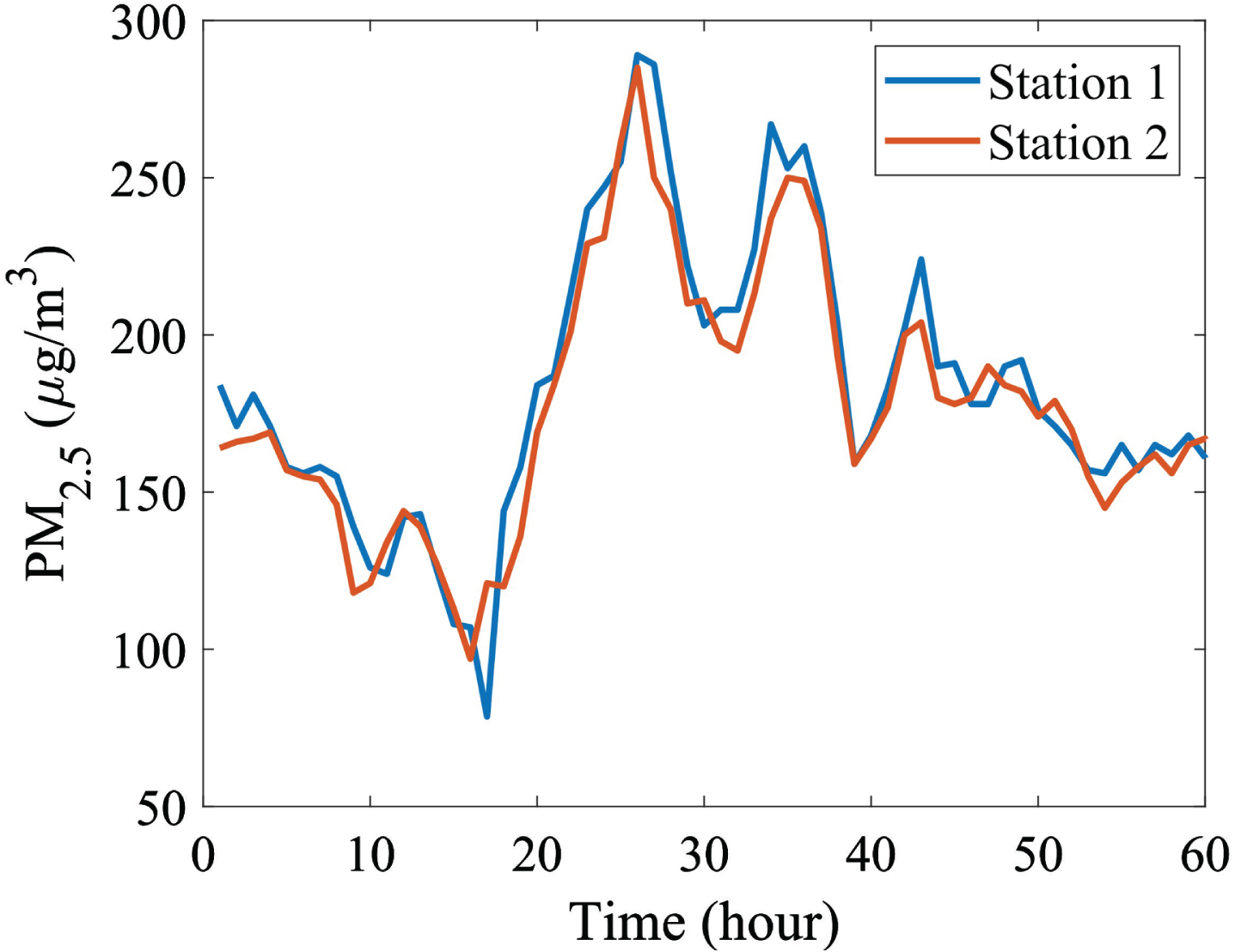
Measured PM_2.5 in two nearby stations.

The PM_2.5 levels at both sites are similar in Fig. 4. On the other hand, Station 1’s trend is often an hour early. Thus, there is a causal connection between these two adjacent stations. As a result, the causation must be examined. A model-free way to quantify causality is Transfer Entropy (TE), which is the information that a cause gives to an effect. TE can measure nonlinear coupling effects and measures the amount of information transferred from one variable to another. Given two concurrently sampled time series X _t and Y _t, t = 1, . . . , T, the transfer entropy from X to Y , denoted as T_{X
→

Y}, can be described as [66]:

Fig. 4

Correlation analysis between various features.

$TE = \sum p (Y_{i + 1}, Y^{i}, X_{i}) \log \frac{p (Y_{i + 1} | Y^{i}, X_{i})}{p (Y_{i + 1} | Y^{i})}$ (8)

In this work, we computed the TE of PM_2.5 between pertinent locations to analyze the causative link and determine how the former affects the latter after a few hours. This technique may also be used to calculate time delays and investigate the causal relationship between PM2.5 and meteorological variables like dew point, air temperature, etc. Then, to better represent the spatial-temporal interactions among sites, we incorporate site timing data, meteorological data, pollutant data, and lagged timing values into the model.

4.4 Reduction of the data dimensionality

A higher dimension of feature space may lead to an increase in complexity and a decrease in the prediction model’s efficacy because of the curse of dimensionality (Lin et al., 2020). To counteract the curse of dimensionality, Principal Components Analysis (PCA) will minimize the dimension of a few selected attributes. In this work, PCA is utilized to reduce the dimension of the data sets while maintaining their features. Principal component analysis (PCA) is widely used to reduce the dimension of data sets while maintaining the highest level of information. By retaining low-order principal components and ignoring high-order principal components, PCA can minimize the number of dimensions. In this way, low-order components may often maintain the most important data features. Condensing a large number of variables into new, uncorrelated variables while maintaining the majority of the data in the larger set is the fundamental strategy of PCA. The new set of variables, known as principal components, is built using the covariance matrix of the original dataset. Additional details on PCA are available in [67].

The chosen features need to be normalized before the PCA dimension reduction process can begin. This is because the projection will attempt to approximate a feature with a high value in the data after it has been projected to the low-dimensional space, which may result in a significant quantity of missing data. The selected data set for this investigation was standardized to [0, 1] by Equation 9, and the normalized data set may be used in subsequent phases. $x^{'} = \frac{x - x_{\min}}{x_{\max} - x_{\min}}$ (9) where x′ is the normalized data; x is the original input data, x_min is the minimum of x, and x_max is the maximum of x.

4.5 Clustering-based pattern partition

Identification of the PWA model begins with feature space partitioning using a clustering-based technique. For identification procedures based on clustering, assessing the “similarity” of data is essential. By enumerating information in dataset elements and characterizing data distribution, the KL Divergence is adopted as a means of evaluating cluster similarity. This paper modified the BIRCH method in [6] for clustering and employed the Kullback-Leibler (KL) Divergence to quantify clusters. Furthermore, because the number of clusters is required by the clustering algorithm, the Davies-Bouldin index (DBI), which calculates the dispersion of each cluster and the dissimilarity between two clusters, is automatically used to estimate the number of clusters. The DBI minimum value can be the number of clusters that will be recommended.

4.5.1 Similarity measure based on KL divergence

The minimum, maximum, and average distance are common similarity metrics across subclasses. It is simple to determine the long-chain subclass using the minimal distance approach. This form offers clear benefits in handling the structure of unequal item density distribution while being at odds with the most well-known spherical structure. Although it is susceptible to noise and isolated points, the greatest distance approach can effectively handle Gaussian clustering. The average distance method strikes a balance between the two approaches. Thus, maximizing the impact of clustering requires a sufficient degree of similarity across classes. Entropy is a metric used in information theory to compare two probability distributions. A metric that has been widely used is called the Kullback-Leibler (KL) divergence. Information divergence, relative entropy, and information for discrimination are all closely related to the KL divergence, a non-symmetric measure of the difference between two probability distributions, p(x) and q(x). For a discrete random variable X, let p(x) and q(x) be its two probability distributions. Then, both p(x) and q(x) sum up to 1, and p(x)>0 and q(x)>0 for any x in X. The KL divergence, denoted as D_KL (p (x) ||q (x)) is defined as: $D_{KL} (p (x) | | q (x)) = \sum_{x \in X} p (x) ln \frac{p (x)}{q (x)}$ (10)

4.5.2 Hierarchical clustering

The improved BIRCH method, which will be employed in this work, was presented in [6]. The whole clustering algorithm consists of two steps, namely initial clustering, and refinement. Firstly, the standard BIRCH algorithm conducts initial clustering on the dataset to obtain smaller clusters. Then, the KL divergence in Equation (10) is used for refinement by merging two clusters with the highest value of the KL divergence into a new cluster. The refinement procedure is conducted iteratively until the required number of clusters is reached. More details about the BIRCH algorithm can be referred to [6].

4.5.3 Determination of the cluster number

The k-means clustering technique that is being explained has to know the number of clusters, hence if there is no pre-knowledge provided, the number of clusters must be calculated. Theoretically, the process of clustering should identify compact, well-defined partitions. It is possible to pick the number of clusters with a lower value of c iteratively by using the cluster validity measure, which provides information on the compactness and separation of clusters [6 , 68]. This study will adopt the Davies-Bouldin index (Davies and Bouldin, 1979) to determine the number of clusters. The ratio of the total within-cluster dispersion to the inter-cluster dissimilarity is known as the Davies-Bouldin Index (DBI), and it is utilized to compare two clusters, C_i and C_j: $DBI = \frac{1}{K} \sum_{i = 1}^{c} R_{i}$ (11)

where R_i is calculated as $R_{i} = max_{i \neq j} \frac{S_{i} + S_{j}}{d_{ij}}$ (12)

S_i denotes the average distance between the data points and the cluster centroid, and d_ij is the distance between clusters i and j centroids. The minimum value of DBI indicates the optimal number of clusters.

4.6 Model order selection and local model parameter estimation

Using the suggested clustering technique to separate the data points, one can then estimate the model’s parameters by minimizing: $min_{Θ} \sum_{k = 1}^{N} {(y_{k} - Θ^{T} \cdot φ_{k})}^{2}$ (13)

The model order represented by n_a and n_b in Equation (3) is estimated by the regularization-based shrinkage using the lasso, which adds a regularization L₁-term to Equation (13) [69]: $min_{Θ} \sum_{k = 1}^{N} {(y_{k} - Θ^{T} \cdot φ_{k})}^{2} + λ \cdot ∥ Θ ∥_{1}$ (14) where λ > 0 is a tuning hyperparameter for a trade-off between model-fit and parameter changes and ∥ · ∥ ₁ is the L₁-norm. The estimation of the model order and local model parameters is shown to be a sparse optimization problem that can be handled by applying global optimization techniques. The most economical model with a manageable prediction error would be chosen as the decision is frequently made using past data or through cross-validation [70].

5 Case study

The proposed method is used in the case study to forecast Beijing’s air pollution. Dongsi is the target station, which the model will forecast (see Fig. 1). Dongsi’s PM_2.5 levels will be predicted using the suggested PWA model using the technique described in section 4. In this part, the PWA model will be identified using the suggested identification method to evaluate the effectiveness of the proposed methodology. In the MATLAB environment, the process was utilized to discover and evaluate several models using an Intel(R) Xeon(R) Gold 5218R CPU operating at 2.10 GHz and 64.0 GB of RAM.

5.1 Model quality evaluation

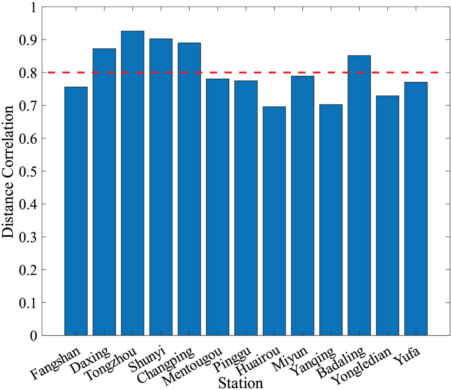
In this study, the suggested model was compared against baselines using the same datasets and scenarios. Three criteria were used to objectively evaluate the model’s quality. They are the correlation coefficient (R), the mean absolute error (MAE), the mean bias error (MBE), the root mean square error (RMSE), the discrepancy ratio (DR) and the scatter index (SI) [71]: $MAE = \sqrt{\frac{\sum_{k = 1}^{N} (\hat{y} (k) - y (k))^{2}}{N}}$ (15) $MBE = \frac{\sum_{k = 1}^{N} (\hat{y} (k) - y (k))}{N}$ (16) $RMSE = \sqrt{\sum_{k = 1}^{N} (\hat{y} (k) - y (k))^{2}}$ (17) $R = \frac{\sum_{k = 1}^{N} (y (k) - \hat{y} (k)) (\hat{y} (k) - \bar{\hat{y}} (k))}{\sqrt{\sum_{k = 1}^{N} (y (k) - \hat{y} (k))^{2} (\hat{y} (k) - \bar{\hat{y}} (k))^{2}}}$ (18) $DR = \log (\hat{y} (k) / y (k)), k = 1, . . ., N$ (19) $SI = \frac{\sqrt{\frac{1}{N} \sum_{k = 1}^{N} (\hat{y} (k) - \bar{\hat{y}} (k)) - {(y (k) - \bar{y} (k))}^{2}}}{\sqrt{\frac{1}{N} \sum_{k = 1}^{N} y (k)}}$ (20) where N is the number of test data, y is the actual value, $\hat{y}$ is the predicted value, y is the mean of the actual values, and $\bar{\hat{y}}$ is the mean of the predicted values. Besides, statistical analysis incl. Violin plot, heatmap, and Taylor diagram [72] is also conducted to compare statistical features between different models.

5.2 Data processing and analysis

Before proposing a PWA model, the data will be preprocessed. First, outliers and missing data will be identified and dealt with using the previously mentioned method. Next, pairwise correlation analysis based on DC will be used to choose the appropriate characteristics. The results of the correlation analysis between different characteristics are presented in Fig. 4. Pairwise correlation analysis based on DC will be used to investigate the correlation information between Dongsi and other stations. As previously mentioned, a higher correlation coefficient value indicates a stronger relationship between observed features and will be selected for additional processing.

The majority of stations in Fig. 5 have a broad correlation with Dongsi. As previously noted, by omitting factors that have weak or no correlation, predicting accuracy can be increased. The criterion of 0.8 is established in this study, and stations that have a correlation coefficient of more than 0.8 will be chosen as highly correlated stations. Stations having a correlation coefficient of less than 0.8 are considered weaker-correlated and will be disregarded. We’ll talk about Daxing, Tongzhou, Shunyi, Changping, and Badaling in the part that follows. The TE of PM_2.5 between pertinent locations is then calculated as part of the causality analysis utilizing TE to establish the several-hour time lag. We computed the TE of PM_2.5 between pairs of factors: Daxing, Tongzhou, Shunyi, Changping, and Badaling to Dongsi to examine the dynamic link between stations. This section also looks into the relationship between dew point and PM_2.5, two meteorological variables. Time delays in the trials range from one to twenty-four hours.

Fig. 5

TE between different stations.

Figure 5 shows that, except Shunyi, which shows a 2 h time lag, TEs reach their peak values with a time lag of 1 h. To better capture spatial-temporal interactions among sites, we then incorporate site timing data, meteorological data, pollutant data, and lagged timing values into the model. PCA has been used to mine the necessary data for the day, except for the predicted value. More than 90% of the data in this study comes from the first three main components of the unique features. Thus, in addition to the anticipated values, these three principal components serve as a substitute for the predictors as part of the input, and the suggested hierarchical technique is then used to cluster the data. The clustering algorithm parameters T and R_max are 0.1 and 20 individually. Because the number of clusters should be pre-defined for the clustering, Algorithm 2 was initialized ten times to select the optimal value. The mean values of the simulation results for DBI suggested that the optimal number should be at c_opt = 3, which is selected in this case study. Next, LASSO optimization is used to jointly estimate the model structure and the sub-model parameters, using the regularization value λ = 10^-2. The proposed technique improved the model order and the parameters of the local models and is implemented in the MATLAB optimization toolbox.

5.3 Baseline models

Predicting air pollutants such as PM_2.5 is primarily used to manage time and provide an early warning system for excessive pollution. Consequently, controlling and mitigating pollution requires a robust forecast model. This section compares and assesses the performance of the PWA model with alternative models. The proposed PWA model is compared in this study to many baseline techniques, including ARIMA, SVM, MLP, LSTM and Bi-LSTM.

Different from those baseline data-driven models, PWA model is defined by partitioning the regression space into a number of polyhedral convex regions and establishing affine models in each region. Globally, PWA model can approximate nonlinear systems and locally, the mapping from regression space to output is piecewise-affine.

5.3.1 ARIMA

The ARIMA model contains three parametric linear parts: autoregression (AR), integration (I), and moving average (MA) model. Often, the ARIMA model is denoted ARIMA (p,D,q), where p is the order of the autoregressive model, D is the degree of differencing, and q is the order of the moving-average model: $\begin{matrix} Δ^{D} y_{t} = c + φ_{1} Δ^{D} y_{t - 1} + \dots + φ_{p} Δ^{D} y_{t - p} + ɛ_{t} + \\ θ_{1} ɛ_{t - 1} + \dots + θ_{q} ɛ_{t - q} \end{matrix}$ (21) where Δ^Dy_t denotes Dth differenced time series, and ɛ_t is an uncorrelated innovation process with a mean of zero.

5.3.2 SVM

Suppose that $ψ (\cdot) : R^{n} \to R^{n_{h}}$ is a nonlinear function that maps input data x into a higher dimensional feature space $R^{n_{h}}$ which may have infinite dimensions. However, in the high dimensional feature space, there always exists a linear function to formulate the nonlinear relationship between input and output data: $f (x) = \sum_{i = 1}^{m} w_{i} ψ (x_{i}, x) + b$ (22) where ψ (x_i, x) are the features of input data after kernel transformation, while w_i and b are coefficients, which are estimated by minimizing regularized risk function as below: $C \frac{1}{N} \sum_{i = 1}^{N} L_{ɛ} (d_{i}, y_{i}) + \frac{1}{2} {∥ w ∥}^{2}$ (23) $L_{ɛ} (d_{i}, y_{i}) = {\begin{matrix} | d_{i} - y_{i} | - ɛ, if | d_{i} - y_{i} | ⩾ ɛ \\ 0, otherwise \end{matrix}$ (24)

where ɛ is a pre-defined parameter, L_ɛ (d_i, y_i) is an ɛ-insensitive loss function, and the $\frac{1}{2} {∥ w ∥}^{2}$ is the term which reflects the flatness of the function. C is then the trade-off between the training error and the model flatness. In order to use SVM to solve a regression problem for predicting air pollutants, the following equation should be calculated: $f (x) = \sum_{i = 1}^{m} (d_{i} - y_{i}) K (x_{i}, x) + b$ (25)

A kernel function K (x_i, x) is used to map the nonlinear data into a feature space where it is linearly separable. In this work, the Gaussian kernel function is adopted as follows: $K (x_{i}, x) = e xp {- \frac{∥ x - x_{i} ∥}{2 σ^{2}}}$ (26) where σ² denotes the width of the Gaussian kernel.

5.3.3 MLP

As a feedforward artificial neural network, the basic structure of an MLP consists of an input layer, one or more hidden layers and an output layer, an activation function, and a set of weights and biases. The input layer distributes the input features to the first hidden layer. The first hidden layer receives the features distributed by the input layer as inputs. The other hidden layers receive the output of each perceptron from the previous layer as inputs. The output layer receives the output of each perceptron of the last hidden layer as inputs. Figure 6 shows an example of an MLP with three layers.

Fig. 6

MLP with three layers.

5.3.4 LSTM

The LSTM network consists of one input layer, one output layer, and a series of recurrently connected hidden layers known as memory blocks. Each block comprises one or more self-recurrent memory cells and three multiplicative units (input, output, and forget gates) that provide continuous analogs of read, write and reset operations for the cells. Figure 7 provides an example of an LSTM memory block, in which i_t, o_t, and f_t mean the activation of the input gate, output gate, and forget gate; C_t and h_t denote the activation vector for each cell and memory block; δ (·) and tanh (·) are the sigmoid function and the tanh function, which are defined as follows: $δ (x) = \frac{1}{1 + \exp (- x)}$ (27)

Fig. 7

Structure of LSTM.

$\tanh (x) = \frac{exp (x) - \exp (- x)}{\exp (- x) + \exp (- x)}$ (28)

5.3.5 Bi-LSTM

Unlike standard LSTM, which can only take features from the past, the Bi-LSTM network consists of two LSTMs: one taking the input in a forward direction and the other in a backward direction. Therefore, the Bi-LSTM network can utilize information from both sides and improve prediction accuracy. The Bi-LSTM layer is shown in Fig. 8.

Fig. 8

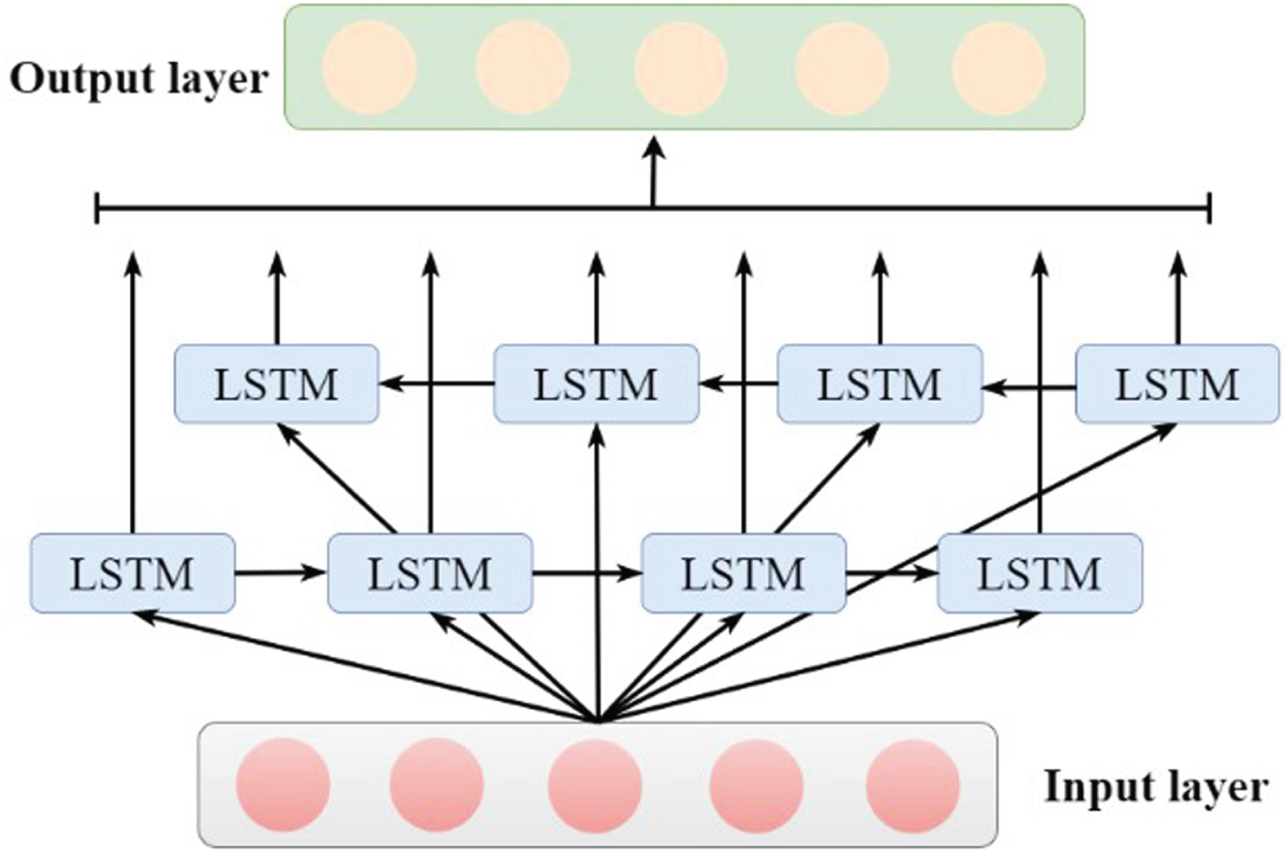
Structure of Bi-LSTM.

5.4 Results and discussion

In this study, several models are applied to identical data sets, but the structure of each model modifies the input sequences. The suggested model is utilized to forecast PM2.5 in this section, and the performance of the PWA model on the testing samples is displayed in Fig. 9.

In Fig. 9, the measurement is shown in the blue line, and the PM_2.5 forecast by the PWA model is shown in the red line. The prediction and the hourly PM_2.5 concentration match exactly. It can accurately represent the effects of PM_2.5 concentration, both static and dynamic, and testing samples show that the model’s prediction and measurement are equivalent. The R between the observed and predicted data for PM_2.5 prediction is 0.99, meaning that the model captured more than 99% of the explained variance. Additionally, it is possible to accurately estimate the majority of peak positions, and the prediction curve closely resembles the real curve. It illustrates how the proposed model may adjust to notable changes in the state. Figure 9 illustrates how the prediction may not always match the peak positions when the PM_2.5 concentration value is higher than 180 g/m³, which leads to more errors than in other situations.

Fig. 9

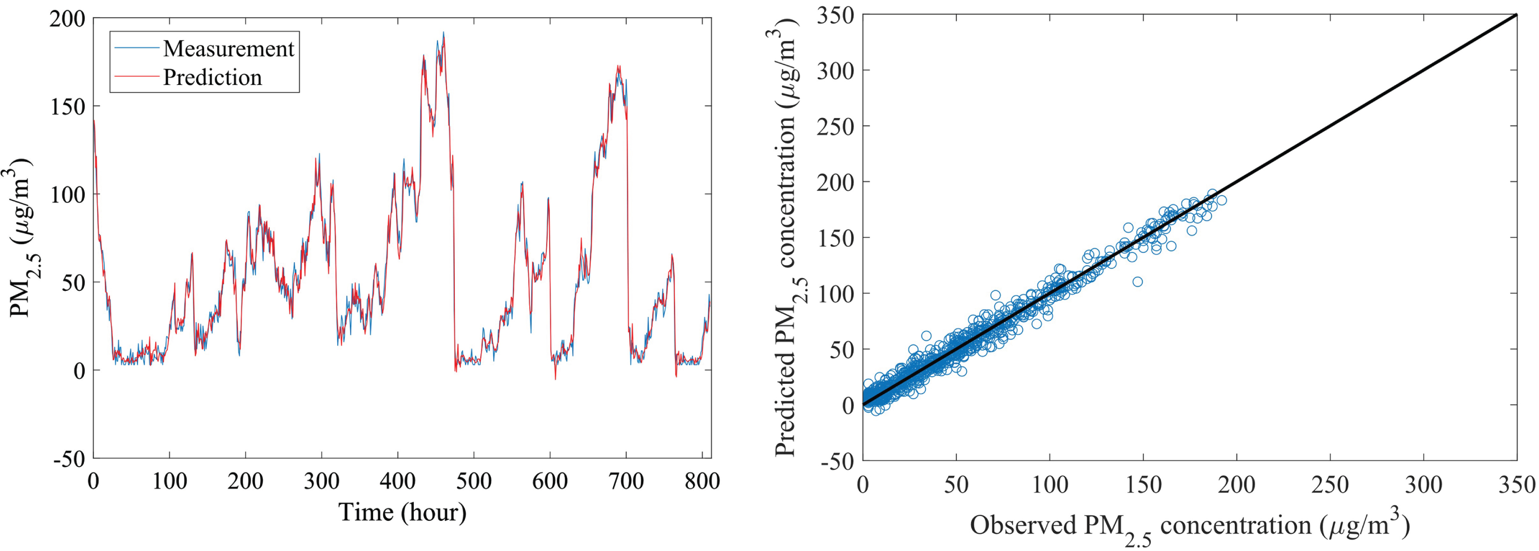
Performance of the PWA model for predicting PM_2.5.

Statistical analysis was also conducted to compare statistical features between different models and Fig. 10 shows the violin plot, heatmap and Taylor diagram for different models. Both violin plot and heatmap show the distribution of Relative Error (RE) and Taylor diagram shows the similarity between models in terms of the correlation, the centered root-mean-square difference and the standard deviations. Results show that the proposed PWA model demonstrated a narrower range of RE values and is closer to the measurement in comparison with baseline models.

Fig. 10

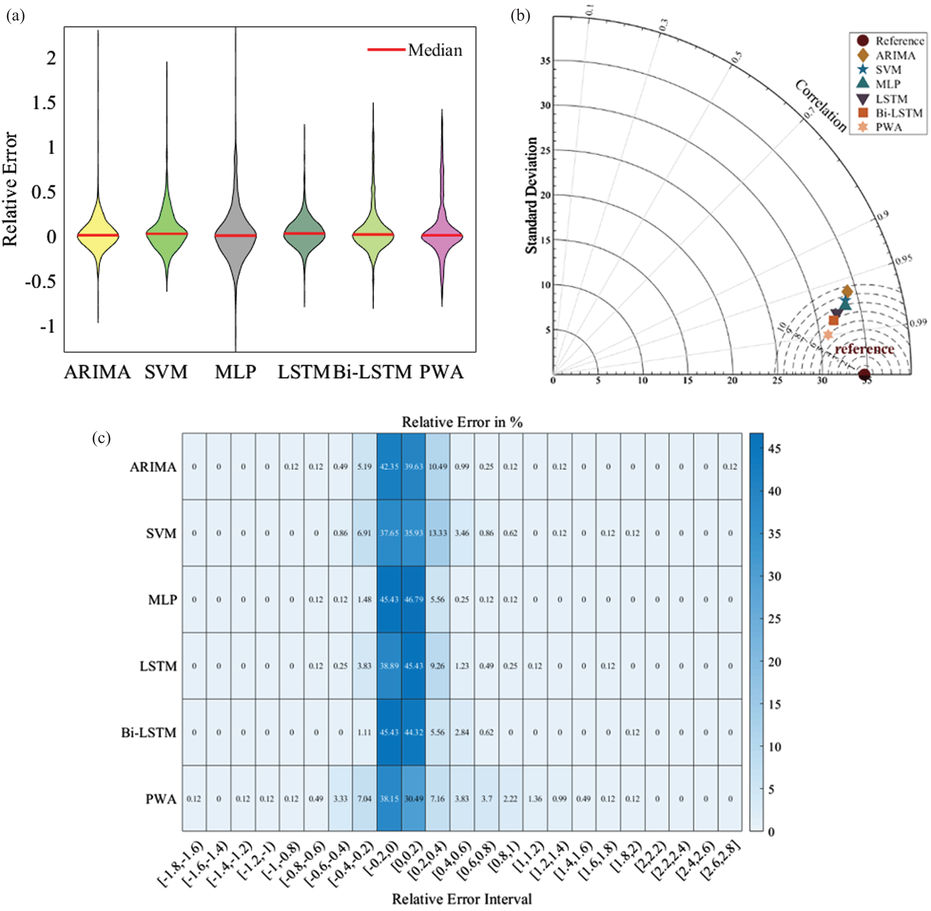
Statistical analysis: (a) Violin plot (b) Taylor diagram (c) heatmap.

Table 1 compares the suggested approach with earlier approaches for PM_2.5 . forecasting. When the model structures are restricted, errors are shown more noticeably by ARIMA, SVM, and the external network MLP, although both deep learning techniques, LSTM and Bi-LSTM, fared better. The MAE, RMSE, R, DR and SI values in Table 1 when compared to other baselines indicate that the proposed model in this work may better describe the features of pollutant concentrations and have a greater prediction capacity. Overall, the proposed model’s performance was sufficient to swiftly adopt extra safety precautions through useful prediction tasks.

Table 1

Comparison of different models for PM_2.5 prediction

Assessment	Model type
ARIMA	SVM	MLP	LSTM	Bi-LSTM	PWA model
MAE	6.28	5.99	5.72	5.34	4.92	4.46
MBE	–0.43	0.45	0.47	–0.03	–0.04	–0.09
RMSE	8.32	7.98	7.61	6.92	6.46	6.28
R	0.95	0.95	0.96	0.97	0.98	0.99
DR	–0.02	–0.02	–0.01	–0.03	–0.01	–0.01
SI	1.23	1.52	1.23	1.29	1.00	0.89

The anticipated values of the PWA model generally match the trend of the observed values. The features selected for this study have a significant impact on air pollution, as evidenced by the efficacy of the recommended method’s predictions. The robustness of the suggested PWA approach is next evaluated utilizing a range of variations by adding white noise (1%, 3%, and 5%) to the time series data. The performance forPM_2.5 concentration prediction under various degrees of additive noise is compared in Table 2. The PWA model’s prediction ability gradually deteriorates as the additive noise level is raised, and its root mean square error (RMSE) marginally increases from 6.28 (in the absence of additive noise) to 7.12 (at the 5% additive noise level). The proposed model is resistant to stochastic disturbances as R remains above 0.97 and predicting accuracy is not greatly affected.

Table 2

Performance comparison under different noise levels for predicting PM_2.5

Assessment	Additive noise level
	0% noise	1% noise	3% noise	5% noise
MAE	4.46	4.76	4.99	5.23
MBE	–0.09	–0.13	–0.12	–0.15
RMSE	6.28	6.51	6.86	7.12
R	0.99	0.98	0.98	0.97
DR	–0.01	–0.03	–0.03	–0.05
SI	0.89	0.91	0.92	1.01

6 Conclusion and outlook

This study employed a unique hierarchical clustering-based identification approach to forecast air contaminants using the PWA model. Next, the recommended technique was applied to Beijing’s air pollution forecasting. The aspects of the problem are summed up first, and then the study field, data sets, and main task are described. The approach comprised the clustering-based identification technique, data preparation, and model structure. Lastly, the Shanghai technique was applied to predict the PM2.5 concentration. The robustness of the model was evaluated at different noise levels. To predict air pollutants, the proposed model was compared with many baseline models.

The results show that the proposed method may successfully and reliably generate higher-quality models appropriate for generating trustworthy management strategies for effective environmental protection as well as early warning of values for excessive air pollution concentrations. The proposed model may be extended to any application utilizing multivariate time series, and future research might use it to anticipate different air pollutants in diverse locations. Future research will target the increase of model quality by considering other potential affecting factors.

Declarations

Consent for publication

All authors gave their consent for publication.

Availability of data and material

The datasets used during the current study are available from the corresponding author upon reasonable request.

Competing interests

The authors declare that they have no known competing financial interests or personal relationships that can have appeared to influence the work reported in this paper.

Funding

This research is supported by the National Natural Science Foundation of China (Grant No.62002255) and the Natural Science Foundation of Shanxi Province, China (Grant No. 20210302123188).

References

Yazdi

M.D.

, et al. The effect of long-term exposure to air pollution and seasonal temperature on hospital admissions with cardiovascular and respiratory disease in the United States: A difference-in-differences analysis, The Science of the Total Environment (2022), 156855.

Atkinson

R.W.

, Kang

, Anderson

H.R.

, Mills

I.C.

and Walton

, Epidemiological time series studies of PM2.5 and daily mortality and hospital admissions: a systematic review and meta-analysis, Thorax 69 (2014), 660–665.

Wang

and Song

, A deep spatial-temporal ensemble model for air quality prediction, Neurocomputing 314 (2018), 198–206.

Zhang

, Ramakrishnan

and Livny

, BIRCH: A new data clustering algorithm and its applications, Data Mining and Knowledge Discovery 1 (1997), 141–182.

Wan

and Yang

, Advanced split BIRCH algorithm in reconfigurable network, J Networks 8 (2013), 2050–2056.

Ren

Z.X.

and Ji

X.X.

, On prediction of air pollutants with Takagi-Sugeno models based on a hierarchical clustering identification method, 31. Art. no, Atmospheric Pollution Research 14(4) (1017), 101731.

Rangel

M.G.L.

, Henríquez

J.R.

, Costa

J.A.M.

and Júnior

J.C.d.L.

, An assessment of dispersing pollutants from the pre-harvest burning of sugarcane in rural areas in the northeast of Brazil, Atmospheric Environment 178 (2018), 265–281.

Yang

, et al. Modification and validation of the Gaussian plume model (GPM) to predict ammonia and particulate matter dispersion, Atmospheric Pollution Research 11 (2020), 1063–1072.

Bray

C.D.

, et al. Evaluating ammonia (NH 3) predictions in the NOAA National Air Quality Forecast Capability (NAQFC) using in-situ aircraft and satellite measurements from the CalNexcampaign, Atmospheric Environment 163 (2017), 65–76.

10.

Lago Kitagawa

Y.K.

, et al. Source apportionment modelling of PM2.5 using CMAQ-ISAM over a tropical coastal-urban area, Atmospheric Pollution Research, 2021.

11.

Thongthammachart

, Araki

, Shimadera

, Eto

, Matsuo

and Kondo

, An integrated model combining random forests and WRF/CMAQ model for high accuracy spatiotemporal PM2.5 predictions in the Kansai region of Japan, Atmospheric Environment 262 (2021), 118620.

12.

Koo

Y.-S.

, Choi

D.-R.

, Kwon

H.Y.

, Jang

Y.-K.

and Han

J.-S.

, Improvement of PM10 prediction in East Asia using inverse modeling, Atmospheric Environment 106 (2015), 318–328.

13.

Saide

P.E.

, et al. Forecasting urban PM10 and PM2.5 pollution episodes in very stable nocturnal conditions and complex terrain using WRF–Chem CO tracer model, Atmospheric Environment 45 (2011), 2769–2780.

14.

Zhou

, et al. Numerical air quality forecasting over eastern China: An operational application of WRF-Chem, Atmospheric Environment 153 (2017), 94–108.

15.

García Nieto

P.J.

, Sánchez Lasheras

, García–Gonzalo

and de Cos Juez

F.J.

, PM10 concentration forecasting in the metropolitan area of Oviedo (Northern Spain) using models based on SVM, MLP, VARMA and ARIMA: A case study, The Science of the Total Environment 621 (2018), 753–761.

16.

Elbayoumi

, Ramli

N.A.

and Yusof

N.F.F.M.

, Development and comparison of regression models and feedforward backpropagation neural network models to predict seasonal indoor PM2.5–10 and PM2.5 concentrations in naturally ventilated schools, Atmospheric Pollution Research 6 (2015), 1013–1023.

17.

Domanska

and Wojtylak

, Application of fuzzy time series models for forecasting pollution concentrations, Expert Syst Appl 39 (2012), 7673–7679.

18.

Yang

, Zhu

, Li

and Li

, A novel combined forecasting system for air pollutants concentration based on fuzzy theory and optimization of aggregation weight, Appl Soft Comput 87 (2020), 105972.

19.

Kaboodvandpour

, Amanollahi

, Qhavami

and Mohammadi

, Assessing the accuracy of multiple regressions, ANFIS and ANN models in predicting dust storm occurrences in Sanandaj, Iran, Natural Hazards 78 (2015), 879–893.

20.

, Jiang

, She

and Lin

, Research on air pollutant concentration prediction method based on self-adaptive neuro-fuzzy weighted extreme learning machine, Environmental Pollution 241 (2018), 1115–1127.

21.

Lin

Y.-C.

, Lee

S.-J.

, Ouyang

C.-S.

and Wu

C.-H.

, Air quality prediction by neuro-fuzzy modeling approach, Appl Soft Comput 86 (2020).

22.

Nabavi-Pelesaraei

, Rafiee

, Mohtasebi

S.S.

, Hosseinzadeh-Bandbafha

, Chau

K.-W.

Comprehensive model of energy, environmental impacts and economic in rice milling factories by coupling adaptive neuro-fuzzy inference system and life cycle assessment, Journal of Cleaner Production, 2019.

23.

Xie

, Ni

J.-Q.

and Su

, A prediction model of ammonia emission from a fattening pig room based on the indoor concentration using adaptive neuro fuzzy inference system, Journal of Hazardous Materials 325 (2017), 301–309.

24.

Zeinalnezhad

, Chofreh

A.G.

, Goni

F.A.

and Klemes

J.J.

, Air pollution prediction using semi-experimental regression model and adaptive neuro-fuzzy inference system, Journal of Cleaner Production 261 (2020), 121218.

25.

Leong

W.C.

, Kelani

R.O.

, Ahmad

Z.A.

Prediction of air pollution index (API) using support vector machine (SVM), Journal of Environmental Chemical Engineering, 2020.

26.

, An

, Zhang

, Zhu

and Zhu

, Prediction of ozone hourly concentrations by support vector machine and kernel extreme learning machine using wavelet transformation and partial least squares methods, Atmospheric Pollution Research 11 (2020), 51–60.

27.

Suleiman

, Tight

M.R.

, Quinn

Applying machine learning methods in managing urban concentrations of traffic-related particulate matter (PM10 and PM2.5), Atmospheric Pollution Research, 2019.

28.

Shamsoddini

, Aboodi

, Karami

Tehran air pollutants prediction based on random forest feature selection method, ISPRS –International Archives of the Photogrammetry, Remote Sensing and Spatial Information Sciences (2017), 483–488.

29.

Yang

, Deng

, Xu

and Wang

, Prediction of hourly PM 2.5 using a space-time support vector regression model, Atmospheric Environment 181 (2018), 12–19.

30.

Alimissis

, Philippopoulos

, Tzanis

C.G.

, Deligiorgi

Spatial estimation of urban air pollution with the use of artificial neural network models, Atmospheric Environment, 2018.

31.

Feng

, Li

, Zhu

, Hou

, Jin

and Wang

, Artificial neural networks forecasting of PM2.5 pollution using air mass trajectory based geographic model and wavelet transformation, Atmospheric Environment 107 (2015), 118–128.

32.

Park

, et al. Predicting PM10 concentration in Seoul metropolitan subway stations using artificial neural network (ANN), Journal of Hazardous Materials 341 (2018), 75–82.

33.

Sayeed

, Choi

, Eslami

, Lops

, Roy

and Jung

, Using a deep convolutional neural network to predict ozone concentrations, 24 hours in advance, Neural Networks: The Official Journal of the International Neural Network Society 121 (2020), 396–408.

34.

, Li

, Karimian

and Liu

, A hybrid model for spatiotemporal forecasting of PM2.5 based on graph convolutional neural network and long short-term memory, The Science of the Total Environment 664 (2019), 1–10.

35.

Chang-Hoi

, et al. Development of a PM2.5 prediction model using a recurrent neural network algorithm for the Seoul metropolitan area, Republic of Korea, Atmospheric Environment 245 (2021), 118021.

36.

Fan

, Li

, Hou

, Feng

X.D.

, Karimian

, Lin

A spatiotemporal prediction framework for air pollution based on deep RNN, ISPRS Annals of the Photogrammetry, Remote Sensing and Spatial Information Sciences (2017), 15–22.

37.

Huang

, Ying

J.J.-C.

and Tseng

V.S.

, Spatio-attention embedded recurrent neural network for air quality prediction, Knowl Based Syst 233 (2021), 107416.

38.

Becerra-Rico

, Aceves-Fernández

M.A.

, Esquivel-Escalante

, Ortega

J.C.P.

Airborne particle pollution predictive model using Gated Recurrent Unit (GRU) deep neural networks, Earth Science Informatics (2020), 1–14.

39.

, Wang

, Ye

and Wang

, Estimating gaseous pollutants from bus emissions: A hybrid model based on GRU and XGBoost, The Science of the Total Environment 783 (2021), 146870.

40.

, Deng

, Wan

H.S.

, Cai

, Pan

A deep learning method to repair atmospheric environmental quality data based on Gaussian diffusion, Journal of Cleaner Production, 2021.

41.

, et al. Development and application of a hybrid long-short term memory –three dimensional variational technique for the improvement of PM2.5 forecasting, The Science of the Total Environment 770 (2021), 144221.

42.

, Ding

, Cheng

J.C.P.

, Jiang

, Wan

A temporal-spatial interpolation and extrapolation method based on geographic Long Short-Term Memory neural network for PM2.5, Journal of Cleaner Production, 2019.

43.

C.-l.

, He

H.-D.

, Song

R.-F.

, Peng

Z.-R.

Prediction of air pollutants on roadside of the elevated roads with combination of pollutants periodicity and deep learning method, Building and Environment, 2021.

44.

Zhao

, Deng

, Cai

and Chen

, Long short-term memory –Fully connected (LSTM-FC) neural network for PM2.5 concentration prediction, Chemosphere 220 (2019), 486–492.

45.

, Li

, Cheng

J.C.P.

, Ding

, Lin

and Xu

, Air quality prediction at new stations using spatially transferred bi-directional long short-term memory network, The Science of the Total Environment 705 (2020), 135771.

46.

Zhang

, Zhang

, Zhao

and Lian

, Constructing a PM2.5 concentration prediction model by combining auto-encoder with Bi-LSTM neural networks, Environ Model Softw 124 (2020), 104600.

47.

Pak

, et al. Deep learning-based PM2.5 prediction considering the spatiotemporal correlations: A case study of Beijing, China, The Science of the Total Environment 699 (2020), 133561.

48.

Zhu

, Deng

, Zhao

and Zheng

, Attention-based parallel networks (APNet) for PM2.5 spatiotemporal prediction, The Science of the Total Environment 769 (2021), 145082.

49.

Zhang

, Zou

, Qin

, Ni

, Mao

and Li

, RCL-Learning: ResNet and convolutional long short-term memory-based spatiotemporal air pollutant concentration prediction model, Expert Syst Appl 207 (2022), 118017.

50.

Zhang

, et al. Deep learning for air pollutant concentration prediction: A review, Atmospheric Environment, 2022.

51.

Yan

, Liao

, Yang

, Sun

, Nong

and Li

, Multi-hour and multi-site air quality index forecasting in Beijing using CNN, LSTM, CNN-LSTM, and spatiotemporal clustering, Expert Syst Appl 169 (2021), 114513.

52.

LeCun

, Bengio

and Hinton

, Deep Learning, Nature 521 (2015), 436–444.

53.

Bartlett

P.L.

, Montanari

and Rakhlin

, Deep learning: a statistical viewpoint, Acta Numerica 30 (2021), 87–201.

54.

Ren

, An optimized excitation signal design for identification of PWA model and application to automotive throttles, Measurement and Control 56(3-4) (2023), 844–856.

55.

Wang

, Song

, Zhao

and Xu

, A PWA model identification method for nonlinear systems using hierarchical clustering based on the gap metric, Comput Chem Eng 138 (2020), 106838.

56.

, Liu

, Qiu

and Buss

, Online Identification of Piecewise Affine Systems Using Integral Concurrent Learning, IEEE Transactions on Circuits and Systems I: Regular Papers 68 (2021), 4324–4336.

57.

Vaezi

and Izadian

, Piecewise Affine System Identification of a Hydraulic Wind Power Transfer System, IEEE Transactions on Control Systems Technology 23 (2015), 2077–2086.

58.

Breschi

, Piga

and Bemporad

, Piecewise affine regression via recursive multiple least squares and multicategory discrimination, Autom 73 (2016), 155–162.

59.

Sindareh-Esfahani

and Pieper

J.K.

, Machine learning–based piecewise affine model of wind turbines during maximum power point tracking, Wind Energy 23 (2020), 404–422.

60.

Yang

, Xiang

, Gao

and Lee

T.H.

, Data-driven identification and control of nonlinear systems using multiple NARMA-L2 models, International Journal of Robust and Nonlinear Control 28 (2018), 3806–3833.

61.

Lauer

On the complexity of piecewise affine system identification, ArXiv, vol. abs/1509.02348, 2015.

62.

Sun

, Hu

, Cai

, Wong

P.K.

and Chen

, Identification of a piecewise affine model for the tire cornering characteristics based on experimental data, Nonlinear Dynamics 101(2) (2020), 857–874.

63.

Song

, Wang

, Ma

and Zhao

, A PWA model identification method based on optimal operating region partition with the output-error minimization for nonlinear systems, Journal of Process Control 88 (2020), 1–9.

64.

Zhang

, Jing

, Liu

, Jiang

and Gu

, A novel PWA lateral dynamics modeling method and switched T-S observer design for vehicle sideslip angle estimation, IEEE Transactions on Industrial Electronics 69(2) (2022), 1847–1857.

65.

Szekely

G.J.

, Rizzo

M.L.

and Bakirov

N.K.

, Measuring and testing dependence by correlation of distances, Annals of Statistics 35(6) (2007), 2769–2794.

66.

Schreiber

, Measuring information transfer, Physical Review Letters 85(2) (2000), 461–464.

67.

Rodgers

J.L.

and Nicewander

W.A.

, Thirteen ways to look at the correlation coefficient, The American Statistician 42 (1988), 59–66.

68.

Ren

, Kroll

, Sofsky

and Laubenstein

, On physical and data-driven modeling of systems with friction: methods and application to automotive throttles, At-Automatisierungstechnik 61(3) (2013), 155–171.

69.

Tibshirani

, Regression Shrinkage and Selection via the Lasso, Journal of the Royal Statistical Society Series b-Methodological 58 (1996), 267–288.

70.

Hastie

T.J.

, Tibshirani

, Friedman

J.H.

The Elements of Statistical Learning: Data Mining, Inference, and Prediction, 2nd Edition, in Springer Series in Statistics, 2005.

71.

Saberi-Movahed

, Najafzadeh

and Mehrpooya

, receiving more accurate predictions for longitudinal dispersion coefficients in water pipelines: Training group method of data handling using extreme learning machine conceptions, Water Resources Management 34 (2020), 529–561.

72.

Najafzadeh

and Anvari

, Long-lead streamflow forecasting using computational intelligence methods while considering uncertainty issue, Environmental Science and Pollution Research 30 (2023), 84474–84490.