Query expansion via learning change sequences

Abstract

Proksch has proved the changed terms of source code negatively affect code search quality. However, current query expansion (QE) methods always ignore it. In this paper we propose a novel QE method based on the semantics of change sequences (QESC). It not only captures which changes occurred by extracting change sequences from Github commits, but also understands why changes occurred by learning sequence semantics with Deep Belief Network (DBN). Thus it could extract relevant terms to expand or irrelevant terms to exclude from the changes semantically similar to a query. Our experimental results show QESC outperforms the existing QE methods by 15–23% in terms of precision on inspecting the first query result.

Keywords

query expansion change sequence DBN

1. Introduction

Query expansion (QE) techniques are widely used for code search. CodeHow [1] expanded a query with online API information on MSDN. QECK [2] expanded a query with Question & Answer (Q&A) pairs on Stack Overflow. However, they always suffer from over-expansion, i.e., expand a query with irrelevant terms confusing the search engine to rank the most relevant result behind all the other results. This is because the expansion terms that should have been relevant will be irrelevant after a code change. As Proksch [3] said, the changed terms of source code have a major effect on many real query cases. Here is an example to illustrate how they affect the search quality.

Figure 1.

Github commit “3eb66fb19ca2aa3d9dce53661f3233b6c 9d3f974”.

Figure 1 shows the Github commit1 of the method “IndexFiles.java”. Two versions of “IndexFiles” before and after the code change are $m_{\textit{AB}}$ and $m_{\textit{AC}}$ , respectively. During this code change, “IndexFiles” retains eleven terms denoted as $A=\{$ docDir docsPath Directory dir FSDirectory open indexPath IndexWriter writer iwc indexDocs $\}$ , deletes two terms denoted as $B=\{$ File, new File $\}$ (at line 78, 88 of $m_{\textit{AB}}$ ) and adds two terms denoted as $C=\{\textit{Path, Paths.get}\}$ (at line 82, 92 of $m_{\textit{AC}}$ ). Then we try three queries to find $m_{\textit{AC}}$ .

If deleted terms of $B$ are added to the query $q(A)$ , the query becomes $q(A+B)$ . The search engine ranks $m_{\textit{AB}}$ higher than $m_{\textit{AC}}$ as $m_{\textit{AB}}$ contains $A$ and $B$ , while $m_{\textit{AC}}$ contains only $A$ . It illustrates QE with deleted terms confuses the search engine.

If deleted terms of $B$ are excluded from the query $q(A)$ , the query becomes $q(A-B)$ . The search engine ranks $m_{\textit{AC}}$ higher than $m_{\textit{AB}}$ as $m_{\textit{AC}}$ contains $A$ but excludes $B$ , while $m_{\textit{AB}}$ contains $A$ and $B$ . It illustrates the exclusion of deleted terms helps the search engine to rank results.

If new terms of $C$ are added to the query $q(A)$ , the query becomes $q(A+C)$ . The search engine ranks $m_{\textit{AC}}$ higher than $m_{\textit{AB}}$ as $m_{\textit{AC}}$ contains $A$ and $C$ , while $m_{\textit{AB}}$ contains only $A$ . It illustrates QE with new terms helps the search engine to rank results.

This example shows the significance of the changed terms of source code. However, it is not enough. We have to understand why the changed terms occurred. As they often occur together with their dependent terms, we think the dependent terms are good indicators to explain why changes occurred, i.e., changed terms could be triggered by their dependent terms.

Figure 2.

Two versions of changed method.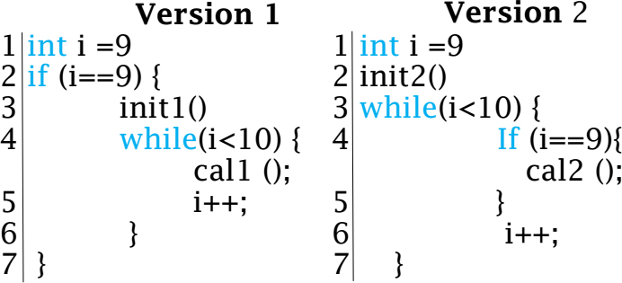

Suppose that a piece of code snippet is changed into version1 and version2 as shown in Fig. 2. Versioin1 has changed terms “init1, cal1” and their dependent terms “if, while”. Versioin2 has changed terms “init2, cal2” and their dependent terms “while, if”. If we infer changed terms based on the traditional occurrence frequencies of dependent terms, we can’t determine if the change terms are “init1, cal1” or “init2, cal2”, because the occurrence frequencies of their dependent terms (“if, while” and “while, if”) are identical. However, the semantic information hidden deeply in source code is different [4]. For version1, the change sequence, containing changed terms and their dependent terms in sequence, is [ $\ldots$ , if, init1, while, cal1, $\ldots$ ]. For version2, the change sequence is [ $\ldots$ , init2, while, if, cal2, $\ldots$ ]. In these two sequences, [if, while] is different from [while, if] semantically. They determine which change terms are inferred by the specific dependent terms precisely: [if, while] for the changed terms “init1, cal1”, [while, if] for the changed terms “init2, cal2”. This example shows the semantics of change sequence could help us to infer the fine-grained changed terms and distinguish one instance of change sequence from another. To learn the sequence semantics, we train Deep Belief Network (DBN) model which could give a semantic vector for each sequences.

In this paper, we propose a novel QE technique with the semantics of change sequences (QESC). It not only captures which changes occurred from Github commits, but also understands why changes occurred with DBN. Therefore, it adds relevant terms to a query and exclude irrelevant terms in a query.

2. Our technique

QESC contains two ends. The back end (Fig. 3I) generates sequences to capture which changes occurred, and build an inference to understand why changes occurred. The front end (Fig. 3II) retrieves method-level results to obtain changes semantically similar to the query.

Figure 3.

Infrastructures of QESC.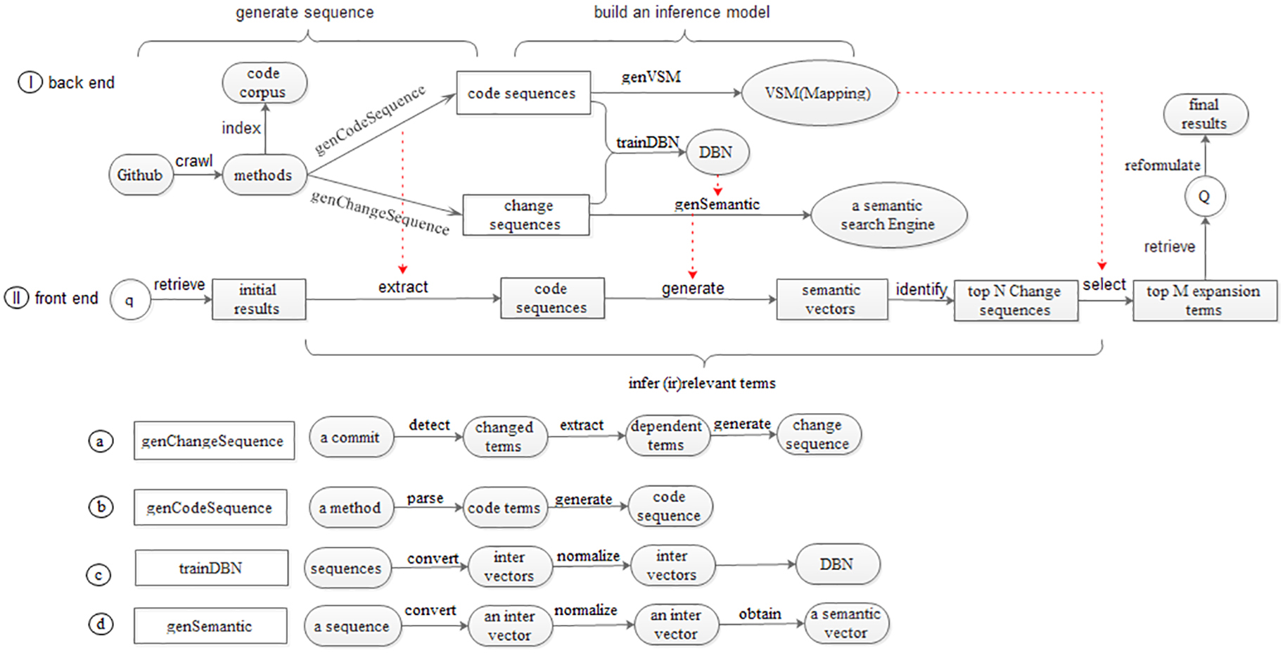

2.1 Generate sequences

2.1.1 Code corpus and change commits

As shown in Fig. 3I, we crawl and parse 590,321 methods from 625 open source projects on GitHub. For each method, we extract code terms with Java Development Tools (JDT2), and convert them into a bag of index words with the text pre-process techniques [5] (e.g., standard tokenization, stop term removal, identifier splitting and stemming). To build a code corpus with Lucene 2.9.1,3 we index all methods as documents containing two fields: index words and method body. On receiving a query, the search engine calculates BM25 textual similarity scores [6] between a query and the index words. According to the scores, query results are ranked in descending order.

For each method in the code corpus, the change commits could be obtained from Github. In the split view, the commit is in the form of the commit ( $m_{1}$ , $m_{2}$ ) where $m_{1}$ and $m_{2}$ are the old version (on the left side) and the new version (on the right side), just like the Github commit of “IndexFiles” (see Section 1). Notably a method has more than one change commit, but not all of commits are collected. We only collect the commit with its feature called “Star” greater than the threshold $\alpha$ ( $\alpha=$ 100). The “Star” represents the attention. Empirically, the more attention the change accepts, the more people are likely to make the change. Statistically, 885,481 commits ( $m_{1}$ , $m_{2}$ ) are collected.

2.1.2 Change sequences

From the commits of each method, we generate change sequences containing changed terms $\Delta$ (the new or the deleted code terms in a code change) and their dependent terms $D$ that are unchanged code terms which are either control or data dependent on $\Delta$ . Here, we define the term as follows.

Definition 1 (Code term). A code term is represented by a triplet of (<label>, <role>, <operation>).

<label> represents the textual information of AST nodes limited to three types: 1) nodes of method invocations and class instance creations; 2) declaration nodes, i.e., method declarations, type declarations, and enum declarations, and 3) control-or data-flow nodes such as while statements, catch clauses, if statements, throw statements, etc. Control-flow nodes are recorded as their statement types, e.g., an if statement is simply recorded as if. <role> has two options that decide if this term is changed or dependent. <operation> has three operations deciding if the term is unchanged, new or deleted in the code change.

In Fig. 3I we describe a function genChangeSequence that inputs a commit of a method, outputting change sequences. The details are as shown in Fig. 3a. It contains three steps: detecting changed terms, extracting dependent terms and generate change sequences.

To detect $\Delta$ , for each commit ( $m_{1}$ , $m_{2}$ ), we use the AST diff tool ChangeDistiller4 which characterizes a method as Abstract Syntax Tree (AST) and computes one-to-one node mappings between the old and the new ASTs for all updated, moved and unchanged nodes. If a node is not in the mappings, it generates a deletion. Otherwise it generates an addition. As a result, the role of the term is “changed”. If a deletion occurs, the operation of the term is “deleted”. If an addition occurs, the operation of the term is “new”. Then we use the static analysis framework Crystal5 [7] to extract $D$ . In this case, the role and the operation of the dependent term are “dependent” and “unchanged”, respectively. Finally, we put $\Delta$ and $D$ together in sequence to generate change sequences.

2.1.3 Code sequences

In Fig. 3I we describe a function called genCodeSequence that inputs a method, outputting a code sequence. The details are as shown in Fig. 3b. It parses three types of code terms from each method in the code corpus, just like genChangeSequence, and put them in sequence to generate the code sequence. As a result, the roles and the operations of all terms are “dependent” and “unchanged”, respectively. Notably in the code sequence all code terms are dependent while in the change sequence some are changed, some are dependent.

2.2 Build an inference model

After obtaining the change and the code sequences, we convert them into vectors of terms, and input these vectors to a deep learning algorithm [8], namely DBN [9], train and learn semantics of sequences automatically. Finally, we build an inference model to infer the fine-grained changes.

2.2.1 Map terms

Since DBN requires input data in the form of integer vectors, we build a mapping between integers and terms, converting the change and the code sequences to integer vectors.

In addition, DBN also requires the lengths of the input vectors must be the same. Since our integer vectors may have different lengths, we append 0 to the integer vectors, making all lengths consistent and equal to the length of the longest vector. Adding zeros does not affect the results, and it is simply a representation transformation making the vectors acceptable by DBN.

To achieve the mapping, in Fig. 3I we describe a function called genVSM that inputs all code sequences, outputting a Vector Space Model (VSM) that not only allocates a unique integer identifier for each non-duplicated term in a code sequence, but also calculates the TFIDF value given a term. TF-IDF is often used to determine the importance of a term for a particular document in the corpus [10].

2.2.2 Train DBN and generate semantics

In Fig. 3I we describe a function called trainDBN which accepts sequences as input and outputs a trained DBN. The details are as shown in Fig. 3c. First we convert the change and the code sequences to integer vectors based on the mapping. However, DBN requires the values of integer vectors ranging from 0 to 1, while data in the integer vectors can have any integer values. To satisfy the input range requirement, we normalize the values in the integer vectors of the sequences by using min-max normalization [11]. With the normalized integer vectors we train DBN while tuning 3 parameters: 1) the number of hidden layers, 2) the number of nodes in each hidden layer, and 3) the number of training iterations. We show how to tune these parameters in Section 3.3.

After training a DBN, in Fig. 3I we also describe a function called genSemantic that inputs a sequence and a trained DBN, outputting a semantic vector as the semantics of the sequence. The details are as shown in Fig. 3d. We map a sequence to an integer vector, normalize it, and feed them into the DBN, obtaining semantics of sequences from the output layer of the DBN. Here, as shown in Fig. 3I, we invoke genSemantic to generate semantic vectors of all change sequences, storing them in a semantic search engine.

2.3 Retrieve query results

We introduce a two-pass retrieval approach to retrieve query results.

First-pass retrieval: On receiving a query $q$ , the search engine produces the initial query results.

Inferring changed terms: Given each initial result, we invoke genCodeSequence to extract its code sequence (see Section 2.1.3). Then we invoke genSemantic to generate its semantic vector (see Section 2.2.2). Next we compare the semantic vector of the initial result against the semantic vectors of all change sequences in the semantic search engine based on the cosine similarity, identifying top- $N$ the most relevant change sequences. Here we set $N$ is 5. From those relevant change sequences, we extract changed terms with the <role> marked “changed” and employ the traditional method, TF-IDF weighting function, to weight scores for the labels of these changed terms. In our work, we utilize the prepared VSM (see Section 2.2.1) to calculate TFIDF values of all labels and select top- $M$ changed terms as expansion terms. Here we set $M$ is 9.

Second-pass retrieval: With the selected changed terms we reformulate the query. If the <operation> of a term is “new”, we see it as relevant term and expand a query with its <label>. If the <operation> of a term is “deleted”, we see it as irrelevant term and remove its <label> in a query. With the reformulated query $Q$ , we perform the second-pass retrieval in the code corpus.

As shown in Fig. 3II, we describe a function called querySearch that inputs a query, outputting a ranked list of the most relevant query results.

3. Evaluation

3.1 Preliminary

3.1.1 Queries generation strategy

To obtain a large number of queries, we propose an artificial queries generation strategy (GenQueries) that inputs a method-level code snippet $m$ , outputting a set of artificial queries $\{q_{1},\ldots,q_{k}\}$ . In this strategy, we 1) extract code terms from $m$ with JDT; 2) perform the random sub-selection of the code terms, hiding the corner cases where the search engine performs particularly well or badly. Here, we pick five out of all code terms as an artificial query randomly at a time; 3) repeat the random sub-selections 3 times to cover different parts of the code snippet for a complete usage; 4) add the changed terms of $m$ , mainly the deleted terms in the code change, to the artificial queries randomly for more realistic evaluation; 5) average the results of these artificial queries to get one representative prediction-quality measure.

3.1.2 Q&R pair generation strategy

To create a large number of benchmark dataset, we propose an artificial Q&R pairs generation strategy (GenQRPair) that inputs a query, a search mode and a ranking mode, outputting a Q&R pair in the form of ( $q,\{r_{1},\ldots,r_{j}\}$ ). Here, $Q$ refers to a query $q, R$ refers to the ranked query results $\{r_{1},\ldots,r_{j}\}$ with each result corresponding to a relevance rating. In this strategy, we 1) perform a query in the search engine with a search mode, and get the query results $\{r_{1},\ldots,r_{j}\}$ ; 2) rank the results with a ranking mode, getting the ranked results $\{r_{1},\ldots,r_{j}\}$ .

For the first step, there are many search modes, such as “Manual”, “None”, “SC”, “CC”, “API” or “CK”.

Manual: a query is performed manually;

None: The search engine performs a query without QE methods;

SC: It inputs a query into querySearch, outputting query results (see Section 2.3).

CC, API or CK: It expands a query with code changes, APIs or crowd knowledge, outputting query results.

For the second step, there are many ranking modes, such as “Manual” or “AutoLabel”.

Manual: the query results are ranked manually;

AutoLabel: the query results are ranked with the automatic Labeling strategy (see Section 3.1.3).

3.1.3 Automatic labeling strategy

To determine whether 2 pieces of code snippets are relevant or not, we propose an automatic labeling strategy (AutoLabel) that inputs 2 pieces of code snippets $m_{A}$ and $m_{B}$ , outputting a relevance rating. In this process, we 1) Calculate the similarity score between $m_{A}$ and $m_{B}$ in Eq. (3.1.3).

$\displaystyle\textit{similarity}(m_{A},m_{B})$ $\displaystyle=\frac{|\textit{matchingNodes}(m_{A},m_{B})|}{\textit{size}(m_{A}% )+\textit{size}(m_{B})}.$ (1)

where matchingNodes( $m_{A}$ , $m_{B}$ ) is the number of matching AST node pairs computed by ChangeDistiller;6 The size( $m_{A}$ ) and size( $m_{B}$ ) is the number of AST nodes in $m_{A}$ and $m_{B}$ , respectively.

2) Based on the similarity score, label the relevance rating with Four-level Likert scale [6], including most relevant, relevant, irrelevant, most irrelevant.

3.1.4 Evaluation method

Given a Q&R pair, in the form of ( $q,\{r_{1},\ldots,r_{j}\}$ ), we propose an automatic evaluation strategy (AE) that inputs a Q&R pair, a search mode and a ranking model, outputting the values of two metrics. In this strategy we 1) input a query in the Q&R pair, a search mode and a ranking model into GenQRPair, getting a Q&R’ pair, in the form of ( $q,\{r^{\prime}_{1},\ldots,r^{\prime}_{j}\}$ ); 2) treat the Q&R pair as “gold standard” and the Q&R’ pair as “final result”, calculating the values of two metrics.

These metrics are $\textit{Accuracy}(A),\textit{Precision}(P)$ [2] and Normalized Discounted Cumulative Gain (NDCG). The P@K is defined as the proportion of the true positives (i.e. the solutions with score 7 or 15) in top-k results for a query [2]. It is calculated as:

$\displaystyle\textit{P@k}=\frac{1}{|Q|}\sum^{|Q|}_{i=1}{\frac{|\textit{% relevant}_{i,k}|}{k}}.$ (2)

where $\textit{relevant}_{i,k}$ represents the relevant solutions for the query $i$ in the top $k$ query results, $Q$ is a set of queries. P@K takes an average on all queries whose relevant answers could be found by inspecting the top $k$ $(k=1,5,10)$ results. A better code search tool should allow users to discover useful solutions by examining fewer results. The higher the value, the better the search is.

NDCG measures the ranking capability of the search algorithm. The algorithm is more relevant when there are more relevant results in the higher positions in the hit list. It is calculated as:

$\displaystyle\textit{NDCG@K}=\frac{\textit{DCG@K}}{\textit{IDCG@K}},$ (3) $\displaystyle\textit{DCG@K}=R_{1}+\sum^{K}_{i=2}{\frac{R_{i}}{\log_{2}i}}.$ (4)

where NDCG@K is DCG@K normalized by IDCG@K. IDCG@K is the ideal DCG@K. Results are sorted by the relevance scores. $R_{1}$ is the relevance score of 1-st result. $R_{i}$ is the relevance score of the $i$ -th result.

3.2 Data preparation

3.2.1 Code corpus

Following the steps in Section 2.1.1, 590,321 method-level code snippets from the 625 open-source projects on Github are indexed. The 625 projects include 6 deeplearning4j libraries,7 8 popular libraries from Anh’s work [8], 295 popular android open-source java projects,8 173 Google Samples labeled with the “java” tag,9 143 Java API examples.10

3.2.2 Benchmark datasets

In the code corpus, all code snippets are sorted in the chronological order. We make 50% most recent code snippets as benchmark dataset. Table 1 shows 1) as a training set, the oldest 60% in the dataset are used for generating VSM and training DBN; 2) as a tuning set, the older 30% are used for generating 265,644 artificial Q&R pairs, tuning 3 parameters of DBN; 3) as a testing set, the newest 10% are used for generating 88,548 artificial Q&R pairs. This is how it happened. Given each code snippet $m$ in the tuning or the testing set, we input it into GenQueries, generating artificial queries $\{q_{1},\ldots,q_{k}\}$ . Then we input each artificial query, the search mode of “None” and the ranking mode of “AutoLabel” into GenQRPair, generating a Q&R pair in the form of ( $q,\{r_{1},\ldots,r_{j}\}$ ).

Table 1
Benchmark dataset

A training set	A tuning set	A testing set
177,096 code snippets	265,644 artificial Q&R pairs	88,548 artificial Q&R pairs

Note that some may not convince such artificial Q&R pairs in two aspects as follows:

They think artificial queries generated from source code couldn’t reflect the real-word situation. To make such queries close to the real queries, we perform the random sub-selection, increase the number of such sub-selections and even average the results of the testing set to get one representative prediction-quality measure (see Section 3.1.1). Especially, we add irrelevant terms (i.e., changed terms with the <operation> marked “deleted”) to the artificial queries. As Proksch et al. [12] reported in 2016, real queries don’t achieve the accurate code search because they contain irrelevant terms that were missing, changed, or got removed in the code change. Besides, a large number of artificial queries could result in valid statistics results to reflect the real-world situations to some extent. Despite a few corner cases, they make up only a small percentage without any impact on measure results.

They think it is not reasonable to rank artificial query results with AutoLabel that implies the relevance score between a query and query results is calculated just with the code term similarity between query results and the original code snippet that generates a query (see Section 3.1.3). Actually, it is reasonable. The underlying idea behind it is that if a piece of code snippet cannot be found with the artificial queries generated by itself, it won’t be found with other queries either easily.

3.3 Model training and tuning

Although we can invoke trainDBN to train DBN (see Section 2.2.2), many DBN applications [13, 14, 15] report that an effective DBN needs well-tuned parameters, i.e., the number of hidden layers, the number of nodes in each hidden layer, and the number of iterations. It implies we need to tune three parameters by conducting experiments with different specific values of the parameters.

Given an experiment, we invoke trainDBN to train DBN with respect to the specific values of the 3 parameters on the training set. Then we invoke genSemantic to generate semantic vectors of all change sequences, storing them in a semantic search engine (see Section 2.2.2). Next we invoke AE that inputs each Q&R pair in the tuning set, the search mode of “SC”, the ranking mode of “AutoLabel”, outputting two metric values (see Section 3.1.4). Based on the values we evaluate the specific values of the parameters. About how to set different values of three parameters, we have two steps as follows.

Step 1: Setting the number of hidden layers and the number of nodes in each layer

Since the number of hidden layers and the number of nodes in each hidden layer interact with each other, we tune these two parameters together. For the number of hidden layers, we experiment with 8 discrete values include 10, 20, 50, 100, 200, 500, 800, and 1,000. For the number of nodes in each hidden layer, we experiment with eight discrete values include 20, 50, 100, 200, 300, 500, 800, and 1,000. When we evaluate these two parameters, we set the number of iterations to 50 and keep it constant. By repeatedly conducting experiments with different values of the parameters, as a result, we choose the number of hidden layers as 10 and the number of nodes in each hidden layer as 100. Thus, the dimension of the semantic vector is 100.

Step 2: Setting the number of iterations

The number of iterations is another important parameter for building an effective DBN. During the training process, DBN adjusts weights to narrow down error rate between reconstructed input data and original input data in each iteration. In general, the bigger the number of iterations, the lower the error rate. However, there is a trade-off between the number of iterations and the time cost. To balance the number of iterations and the time cost, we conduct experiments with 10 discrete values for the number of iterations. The values range from 1 to 1,000. We use error rate to evaluate this parameter. By repeatedly conducting experiments with different values of the parameters, as a result, we set the number of iterations to 200, with which the average error rate is about 0.134 and the time cost is about 23 seconds.

3.4 Setup

3.4.1 QESC

For all code snippets in the training set, according to the name of each method-level code snippet, we extract their Github commits. Then we invoke genChangeSequence and genCodeSequence to extract their change sequences (see Section 2.1.2) and code sequences (see Section 2.1.3), respectively. Based on these sequences, we invoke genVSM to generate VSM containing a mapping (see Section 2.2.1). With the code and the change sequences, we train and tune DBN as Section 3.3 said. After preparing VSM, the trained DBN with the best specific values of the parameters, we invoke querySearch that inputs a query, outputting query results (see Section 2.3). Actually, this is the search mode of “SC” described in Section 3.1.2.

3.4.2 QECC

In order to evaluate whether DBN, a deep learning, is useful for code search or not, we make QECC (omitting DBN) to compare with QESC (using DBN). Actually, QECC is also proposed by us in 2018 [16]. It is similar to QESC in terms of principle, but the inference model is different. The former leverages a statistical method while the latter leverages a deep learning.

First, QESC trains DBN that considers the semantics of the change sequence (see Section 2.1.2). However, QECC trains a $Pr(\Delta|C)$ that is the probability of changed terms $\Delta$ occurring given dependent terms $C$ . In this process, it applies EM algorithm to ( $\Delta,C$ ) pairs, considering the number of times that $\Delta$ and C appeared together. Note that the change sequence is different from the ( $\Delta,C$ ) pair. In the former $\Delta$ and $C$ are put together in order while in the latter $\Delta$ are separated from $C$ . For example, QESC accepts the change sequence of $m_{\textit{AB}}$ (see Section 2.1.2) while QECC accepts the ( $\Delta,C$ ) pair from $m_{\textit{AB}}$ . The pair is {{(File, changed, deleted), (new File, changed, deleted) (exists, changed, deleted), (canRead, changed, deleted), (getAbsolutePath, changed, deleted), (new File, changed, deleted)}, {(if, dependent, unchanged), (try, dependent, unchanged), (Directory, dependent, unchanged), (FSDirecetory.open, dependent, unchanged), (IndexWriter, dependent, unchanged), (new IndexWriter, dependent, unchanged), (indexDocs, dependent, unchanged)}}.

Second, QESC infers expansion terms for a query based the semantic similarity between initial results and each change sequence (see Section 2.3). QECC infers expansion terms based on $Pr(\Delta|C)$ : 1) extract code terms as $C$ from the top-5 initial results; 2) infer the top 9 of $\Delta$ of being triggered by these $C$ with some probability. Actually, this is the search mode of “CC” described in Section 3.1.2.

3.4.3 CodeHow

According to the name of each method in the code corpus, we extracted API name and description (i.e., FQN, summary and remarks) from MSDN and other online documentations11 (i.e., “Workbench User Guide”, “Java Development User Guide”, “PDE Guide”, “Platform Plug-in Developer Guide” and “JDT Plug-in Developer Guide”). After indexing them, we implement CodeHow that identifies the top 5 of relevant APIs that match a query: 1) compute the similarity between the API name and the query as well as the similarity between the description and the query; 2) combine two similarity values and 3) return the potentially relevant APIs. With the identified APIs and the original query it generates Boolean query expressions and retrieve query results with Extended Boolean model (EBM) [17]. Actually, this is the search mode of “API” described in Section 3.1.2.

3.4.4 QECK

According to the name of each method in the code corpus, we collected the questions with the “android, java” tags posted by users and the accepted answer with “AcceptedAnswer” from the Stack Exchange Data Dump,12 and generated Q&A pairs consisting of words and SO score. The words are the text in question and answer. The SO score is a weighted mean value between the individual scores of the question and the answer voted by crowd. After indexing Q&A pairs, we implement QECK that identifies the top 5 of relevant Q&A pairs that match a query: 1) compute SO score and Lucene score that is the similarity between the words of Q&A pair and the query; 2) combine 2 similarity values and 3) return the potentially relevant Q&A pairs as Pseudo Relevance Feedback (PRF) documents. From these documents we extract the top 9 of the software specific words with the high weighting of TF-IDF. With the identified words we expand the original query and retrieve query results with BM25. Actually, this is the search mode of “CK” described in Section 3.1.2.

3.5 Results and analysis

Following the steps in Section 3.4, we implement QESC, QECC, CodeHow and QECK, conducting experiments to answer three research questions (RQs). For drawing confident conclusions whether our approach is really effective, we conduct a statistical test to compare the mean values of two metrics in the experiments. Specifically, we conduct the 2-sided Wilcoxon’s signed rank test between two results. When comparing each pair of results, the primary null hypothesis is that there is no statistical difference in the performance between two results. Here, we employ the 95 percent confidence level (i.e., the $p$ -values below 0.05 are considered significant).

RQ1: Is QESC better than the state-of-the-art QE methods when facing the queries that none has executed?

We employ AE (see Section 3.1.4) that accepts each Q&R pair in the artificial testing set, the search mode of “SC” for QESC, “API” for CodeHow, “CK” for QECK, and the ranking mode of “AutoLabel” as input, outputting the values of two metrics. Based on the values we compare QESC against CodeHow and QECK.

From Table 2, we can see all $p$ -values less than 0.05. So we reject the null hypothesis, accepting the alternative hypothesis that there is a statistically significant difference in the mean values of the two metrics. The performance of QESC is better than the performance of CodeHow and QECK. In terms of the mean value of Precision, QESC is better than CodeHow and QECK by 23% and 15% P@1, 32% and 22% P@5. In terms of the mean value of Accuracy, QESC is better than CodeHow and QECK by 18% and 10% A@1, 27% and 18% A@5. In terms of the mean value of NDCG, QESC is better than CodeHow and QECK by 27% and 14% NDCG@1, 32% and 22% NDCG@5. Note that the precision of CodeHow and QECK is lower in the previous papers [1, 2] because the relevance scores are calculated according to Eq. (3.1.3) instead of being labeled by the recruited experts.

Table 2
Mean of two metrics of three methods

Metrics	Approaches	Top 1	Top 5
Precision	QESC	0.816 ${}^{0.004,0.003}$	0.795 ${}^{0.003,0.002}$
	QECK	0.712	0.651
	CodeHow	0.665	0.601
Accuracy	QESC	0.773 ${}^{0.002,0.003}$	0.762 ${}^{.002,0.002}$
	QECK	0.702	0.647
	CodeHow	0.654	0.598
NDCG	QESC	0.8102 ${}^{0.002,0.003}$	0.7887 ${}^{0.001,0.002}$
	QECK	0.7102	0.6475
	CodeHow	0.6389	0.5985

The “ $+$ ” refers to two $p$ -values are less than 0.05. The first is calculated among the pairwise comparison for QESC and QECK; the second is calculated among that for QESC and CodeHow.

This is a fair comparison because none of QESC, CodeHow and QECK has ever executed these 88,548 artificial queries. The reasonable results show QESC is better than others. Take $m_{\textit{AC}}$ in Fig. 1 for example. Give a random artificial query “Directory, IndexWriter, Document, File”. It contains 3 relevant terms {“Directory”, “IndexWriter”, “Document”} that the method contains and 1 irrelevant term “File” that the method does not contain. The former helps the search engine to recommend $m_{\textit{AC}}$ , while the latter confuses the search engine to miss $m_{\textit{AC}}$ .

Table 3

Three expansion queries generated by CodeHow, QECK and QESC

	Expansion queries
	Relevant terms	Irrelevant terms
CodeHow	Directory, IndexWriter, Document	File, $+$ new File
QECK	Directory, IndexWriter, Document	File, $+$ search, $+$ filed
QESC	Directory, IndexWriter, Document $+$ Path, $+$ Paths.get	File, $-$ File, $-$ new File

Table 3 lists how to expand a query to recommend $m_{\textit{AC}}$ with CodeHow, QECK and QESC, respectively. CodeHow identified an irrelevant term “ $+$ new File” from the description of the online documentation13 and generate an expansion query containing three relevant terms and two irrelevant terms. QECK identified two irrelevant terms “ $+$ search, $+$ filed” from the PRFs of Q&A pairs on Stack Overflow14 and generate an expansion query containing three relevant terms and three irrelevant terms. These expansion queries perform worse than the original query as they have more irrelevant terms. However, QESC performs best because it identified “ $+$ Path, $+$ Paths.get, $-$ File, $-$ new File” from the changed terms and generate an expansion query containing five relevant terms and 0 irrelevant terms.

This example illustrates 1) QESC can exclude the irrelevant terms while CodeHow and QECK cannot; 2) QESC adds relevant terms while CodeHow and QECK would add irrelevant terms. This is because the terms provided by QESC originate from the inside of the method while the terms provided by CodeHow and QECK originate from the outside of the method, such as MSDN and Stack Overflow. It explains why QESC is better than CodeHow and QECK.

RQ2: Is the DBN, a deep learning, effective?

Answers to this research question will shed light on whether DBN, a deep learning, is useful for code search or not. Thus we compare QESC (using DBN) against QECC (omitting DBN). We employ AE that accepts each Q&R pair in the artificial testing set, the search mode of “SC” for QESC, “CC” for QECC, and the ranking mode of “AutoLabel” as input, outputting the values of two metrics. Based on the values we compare QESC against QECC.

Table 4

The performance of the baseline QESR, vs. the performance of the QECC

Metrics	Approaches	Testing set
		Top 1	Top 5
Precision	QESC	0.824 ${}^{+0.004}$	0.801 ${}^{+0.002}$
	QECC	0.788	0.767
Accuracy	QESC	0.795 ${}^{+0.003}$	0.786 ${}^{+0.002}$
	QECC	0.771	0.752
NDCG	QESC	0.8189 ${}^{+0.003}$	0.7987 ${}^{+0.002}$
	QECC	0.7905	0.7521

The “ $+$ ” refers to the $p$ -value is less than 0.05 among the pairwise comparison for each QE method.

From Table 4, we can see all $p$ -values less than 0.05. It illustrates there is a statistically significant difference in the mean values of the two metrics. For the artificial testing set, QESC performs better than QECC. These results indicate that the use of DBN to infer fine-grained changed terms could improve the ranking performance of the code recommendation. This is reasonable because the DBN-based QESC considers the semantics of change sequence while the EM-based QECC cannot distinguish semantic meanings of different orders of terms. It considers only the occurrence frequencies that changed terms and dependent terms appeared together.

3.6 Limitation

Although QESC is effective, some methods are still difficult to find. For example, some methods have only a few changed terms to expand, which do not work in QE. For another example, some methods have no changed terms to expand. Maybe the methods have no change commits on Github as they have never evolved. Maybe the methods have change commits but these commits are not popular and omitted directly, such as the method “openDirectory”. When we judge what kind of commits could be collected, we consider only the “Star” but not time interval which cannot reflect the attention effectively. Some new commits are not always cool. Instead, the “Star” can reflect the attention. The more attention the change accepts, the more people are likely to make the change. In this paper, we collect the commits with “Star” greater than the threshold $\alpha$ . In the future, we will adjust $\alpha$ to achieve the best performance.

4. Related work

Recently, many deep learning methods have been proposed [18] applied deep convolutional neural networks into image-net classification [19] focused on diagnosing gear faults in induction machine systems [20] put emphasis on LSTM recurrent networks itself. Therefore, we use deep learning for solving the problem of code search in software engineering.

In 2018, we proposed a novel QE technique with code changes (QECC) [16]. Now, by employing DBN a deep learning, we propose a novel QE technique with the semantics of change sequences (QESC). Although they apply the regularity of code changes to QE methods, there are five differences.

The original intention is different. Code changes in QECC are used to infer users’ coding intent (i.e., what users want). However, those in QESC are used to avoid the over-expansion (i.e., expand a query with irrelevant terms).

The effect of QE is different. QECC only add the expansion terms that represent user needs. However, QESC not only add relevant expansion terms, but also exclude irrelevant ones in the original query.

The training data is different. Although both of them need to detect changed terms and extract dependent terms, QECC exploits (changes, contexts) pairs while QESC generates code sequences. In a pair, changes are separated from contexts. A code change and a change context are defined as a triplet of (<operation kind>, <AST node type>, <label>) and a tuple of (<AST node type>, <label>, <change>, <distance>), respectively. In a code sequence, changes and contexts are both put together in order. They are uniformly defined as a triplet of (<label>, <role>, <operation>). In addition, for the node edits, QECC considers only inserts, updates and moves. Beside these, QESC also considers deletes.

The training method is different. QECC trains a statistical word alignment model Pr (changes|contexts) by applying a machine learning (ML) algorithm called expectation maximization (EM) algorithm. However, QESC trains DBN model by applying a deep learning algorithm. As a result, QECC only capture which changes occurred while QESC also understand why changes occurred by learning the semantics of code sequences. Faced with “if, while” and “while, if”, only QESC could distinguish them. QECC can’t because the occurrence frequencies of “if, while” and “while, if” are identical.

The inferring of changes is different. Give initial results, QECC extracts code terms from them, seeing them as dependent terms to infer changed terms with Pr (changes|contexts). In the same case, QESC converts them into semantic vectors with DBN, inferring the changes semantically similar to them.

5. Conclusion

We propose QESC to apply the change sequences to QE methods. It expands the query with relevant terms and remove irrelevant terms in the query.

Footnotes

https://github.com/apache/lucene-solr/commit/3eb66fb19ca2aa 3d9dce53661f3233b6c9d3f974?diff=split#diff-b8ac31d6d60f4864 d5987fbb875503b9.

https://github.com/eclipse/eclipse.jdt.core.

http://central.maven.org/maven2/org/apache/lucene/lucene-core/2.9.1/lucene-core-2.9.1.jar.

https://bitbucket.org/sealuzh/tools-changedistiller/overview.

https://code.google.com/archive/p/crystalsaf/.

https://bitbucket.org/sealuzh/tools-changedistiller/overview.

https://github.com/deeplearning4j.

https://github.com/Trinea/android-open-project/blob/master/ English%20Version/README.md.

https://github.com/googlesamples?language=java.

http://www.java2s.com/Code/JavaAPI/CatalogJavaAPI.htm.

http://www.eclipse.org/documentation/.

http://archive.org/download/stackexchange.

https://lucene.apache.org/core/2_9_4/api/all/org/apache/lucene/ store/FSDirectory.html.

http://stackoverflow.com/questions/33825369/using-apache-lucene-to-search.

References

Zhang

H.Y.

Lou

J.G.

Wang

S.W.

Zhang

D.M.

and Zhao

J.J.

, CodeHow: Effective code search based on API Understanding and extended boolean model (E), in: Proc 30th IEEE/ACM International Conference on Automated Software Engineering (ASE), Lincoln, NE, USA, (2015), 260–270.

Nie

Jiang

Ren

Sun

and Li

, Query expansion based on crowd knowledge for code search, IEEE Transactions on Services Computing, (2016), 771–783.

Proksch

Amann

Nadi

and Mezimi

, Evaluating the evaluations of code recommender systems: A reality check, in: Proc of 31st IEEE/ACM International Conference on Automated Software Engineering, Singapore, (2016), 111–121.

White

and Vendome

Linares-Vàsquez

and Poshyvanyk

, Toward deep learning software repositories, in: Proc the 12th Working Conference on Mining Software Repositories, Florence, Italy, (2015), 334–345.

Sun

Liu

and Zhu

, Empirical studies on the NLP techniques for source code data preprocessing, in: Proc 3rd International Workshop on Evidential Assessment of Software Technologies, Nanjing, China, (2014), 32–39.

Manning

C.D.

Raghavan

and Schtze

, Introduction to information retrieval, Cambridge University Press, 2008.

Fluri

Wursch

Pinzger

and Gall

H.C.

, Change distilling – tree differencing for fine-grained source code change extraction, IEEE Transactions on Software Engineering SE-33(11) (2007).

Hinton

G.E.

and Salakhutdinov

R.R.

, Reducing the dimensionality of data with neural networks, American Association for the Advancement of Science, (2006), 504–507.

Hinton

G.E.

Osindero

and The

Yee Whye

, A fast learning algorithm for deep belief nets, Neural Computation (2006), 1527–1554.

10.

Haiduc

Bavota

Marcus

Oliveto

Lucia

A.D.

and Menzies

, Automatic query reformulations for text retrieval in software engineering, in: Proc (2013) International Conference on Software Engineering, San Francisco, CA, USA (2013), 842–851.

11.

Witten

I.H.

and Frank

, Data mining: Practical machine learning tools and techniques, Morgan Kaufmann Series, (2005).

12.

Proksch

Amann

Nadi

and Mezimi

, Evaluating the evaluations of code recommender systems: A reality check, in: Proc of 31st IEEE/ACM International Conference on Automated Software Engineering, Singapore, (2016), 111–121.

13.

Ciresan

Meier

and Schmidhuber

, Multi-column deep neural networks for image classification, in: Proc (2012) IEEE Conference on Computer Vision and Pattern Recognition (CVPR), Washington, DC, USA, (2012), 3642–3649.

14.

Krizhevsky

Sutskever

and Hinton

G.E.

, Imagenet classification with deep convolutional neural networks, Communications of the ACM, (2017), 84–90.

15.

Mohamed

A.-R.

Dahl

G.E.

and Hinton

, Acoustic modeling using deep belief networks, IEEE Transactions on Audio, Speech, and Language Processing, (2012), 14–22.

16.

Huang

Yang

Zhan

Wan

and Wu

, Query expansion based on statistical learning from code changes, Softw Pract Exper (2018), 1–19. doi: 10.1002/spe.2574.

17.

Raychev

Vechev

M.T.

, Eran Yahav, code completion with statistical language models, in: Proc the 35th ACM SIGPLAN Conference on Programming Language Design and Implementation, Edinburgh, UK (2014), 419–428.

18.

Krizhevsky

Sutskever

and Hinton

G.E.

, Imagenet classification with deep convolutional neural networks, 25th International Conference on Neural Information Processing Systems (2012), 1097–1105.

19.

Razavi-Far

Hallaji

and Farajzadeh-Zanjani

, Information fusion and semi-supervised deep learning scheme for diagnosing gear faults in induction machine systems, IEEE Transactions on Industrial Electronics (2018).

20.

Gers

F.A.

and Schmidhuber

, LSTM recurrent networks learn simple context-free and context-sensitive languages, IEEE Transactions on Neural Networks 12(6) (2001), 1333–1340.

Query expansion via learning change sequences

Abstract

Keywords

1. Introduction

2.1.1 Code corpus and change commits

2.1.2 Change sequences

2.1.3 Code sequences

2.2 Build an inference model

2.2.1 Map terms

2.2.2 Train DBN and generate semantics

2.3 Retrieve query results

3. Evaluation

3.1 Preliminary

3.1.1 Queries generation strategy

3.1.2 Q&R pair generation strategy

3.1.3 Automatic labeling strategy

3.2.1 Code corpus

3.2.2 Benchmark datasets

Table 1 Benchmark dataset

Step 1: Setting the number of hidden layers and the number of nodes in each layer

Step 2: Setting the number of iterations

3.4 Setup

3.4.1 QESC

3.4.2 QECC

3.4.3 CodeHow

3.4.4 QECK

3.5 Results and analysis

Table 2 Mean of two metrics of three methods

4. Related work

5. Conclusion

Footnotes

References

Table 1
Benchmark dataset

Table 2
Mean of two metrics of three methods