Software fault prediction using machine learning techniques with metric thresholds

Abstract

BACKGROUND:

Fault data is vital to predicting the fault-proneness in large systems. Predicting faulty classes helps in allocating the appropriate testing resources for future releases. However, current fault data face challenges such as unlabeled instances and data imbalance. These challenges degrade the performance of the prediction models. Data imbalance happens because the majority of classes are labeled as not faulty whereas the minority of classes are labeled as faulty.

AIM:

The research proposes to improve fault prediction using software metrics in combination with threshold values. Statistical techniques are proposed to improve the quality of the datasets and therefore the quality of the fault prediction.

METHOD:

Threshold values of object-oriented metrics are used to label classes as faulty to improve the fault prediction models The resulting datasets are used to build prediction models using five machine learning techniques. The use of threshold values is validated on ten large object-oriented systems.

RESULTS:

The models are built for the datasets with and without the use of thresholds. The combination of thresholds with machine learning has improved the fault prediction models significantly for the five classifiers.

CONCLUSION:

Threshold values can be used to label software classes as fault-prone and can be used to improve machine learners in predicting the fault-prone classes.

Keywords

Fault prediction software metrics threshold values machine learning

1. Introduction

Software testing is a challenging activity that is necessary to find faults in systems. Software testing is a costly activity that requires a large amount of software production effort (i.e., between 50 to 70 percent) [3, 12]. In addition, software systems are becoming larger and more complex. Therefore, software quality assurance efforts are increasing and software testing teams need to be larger. Furthermore, the exhaustive testing of software is impractical for large systems. Therefore, software testers need to allocate testing resources effectively and efficiently. Software testers need to use code analysis tools to measure fault-proneness of classes using software metrics and direct the testing efforts to such classes.

The fault-proneness refers to the probability of faults in a particular class. The fault-proneness models are either machine learning or statistical models. Building fault-proneness prediction models requires a dependent variable (i.e., fault-proneness) and many independent variables (i.e., software metrics). Instances of values closer to 1 are more fault-prone than otherwise. Therefore, the dependent variable is a binary variable of two values, faulty for the classes that have at least one fault and non-faulty otherwise. The independent variables are the software metrics that measure the internal software quality. Improving the performance of fault-prediction models helps the software testers in allocating resources more accurately.

A static analyzer collects quantitative measures of the internal software quality such as complexity, coupling, cohesion, inheritance, and class responsibility. Internal quality of software systems is measured using metrics that were linked with many external quality attributes such as fault-proneness. Software metrics were validated as predictors of fault-proneness of code using machine learning and regression techniques [2, 22, 23, 24, 34, 40, 47, 49]. Examples of prediction models include decision trees [12, 15, 35], naïve Bayes [52], and logistic regression [2].

Most reported fault data in literature show imbalance, i.e., faulty classes are the minority while the majority of classes are not faulty [38, 48]. One important reason of data imbalance could be that software testing coverage was incomplete or that the time was not sufficient for the testing team. Therefore, many faults are expected in systems and many classes can be labeled as fault-prone even if these classes were not reported in the first place as such by the developers and the testers. If the fault-prone classes can be identified amongst the unlabeled classes, improvements are expected on reducing the data imbalance and consequently, the fault prediction performance can be improved as well. The classes that are complex and fault-prone but not reported as such hinder the fault-prediction models. Therefore, there is a need to improve the datasets, which improves the performance of prediction.

Software components were found correlated with high measurements such as high coupling, high lack of cohesion, large complexity, and large classes. High measurements increase the fault-proneness of classes. Software thresholds can provide these indicators to the fault prediction models. Thresholds for these metrics can be used to identify the classes that are highly complex and fault-prone.

Metric thresholds were identified in the literature as reference points at which fault-proneness increases [14, 41, 50]. Therefore, thresholds are usually used to label classes as faulty for further quality investigation. In previous literature, all derived thresholds were set such that large values are fault-prone whereas smaller values are not. Threshold values are used in this work to improve fault-prediction performance. The datasets quality is improved by identifying the classes where metric values exceed particular thresholds that were reported as non-faulty.

There are many threshold identification techniques that were reported in the literature. In this research, three threshold identification techniques [14, 41, 50] are used to mark classes as faulty if they exceed threshold values. These techniques derive thresholds for software metrics using statistical parameters such as the mean and the standard deviation. These techniques are selected for various reasons, first, the three techniques were validated on a large benchmark. Most systems used as benchmarks were large in size and coming from different application domains. Second, these techniques are simple and easy to use by software engineers. Third, these techniques are easy to repeat on future data.

The proposed research improves the quality of fault data. Threshold values are used to target the classes that are marked as not faulty. The non-faulty instances are separated using thresholds into two parts: classes that are larger than thresholds and classes that are lower than thresholds. Classes selected by thresholds are unlabeled and removed from the dataset waiting for further investigation. The labeled datasets are used to build fault prediction models. These models are then used to test the unlabeled instances. The results of testing are used to improve the fault datasets. An instance that is predicted as faulty is labeled as such, whereas the instances that are predicted as not faulty are kept non-faulty.

Our contribution to fault prediction research is summarized as follows:

•
We propose easy to use three threshold identification techniques to label classes and to reduce data imbalance.
•
The results of threshold identification techniques are used to improve the quality of the datasets.
•
The improved datasets are used to build five fault-prediction models.

Therefore, this research answers three research questions:

RQ1: Does traditional learning suffer under data imbalance? RQ2: Does using thresholds reduce the data imbalance in fault data? RQ3: Does using thresholds improve the fault prediction models?

In the rest of the paper, the related work is discussed in section two. Study design and research methodology are described in Section three. Results analysis is presented in section four to answer the three research questions. Study limitations are briefed in section five. Finally, the work is concluded in section six.
2. Related work

This research combines the use of fault prediction with the threshold values to improve the fault-prediction models on imbalanced datasets. In the following, we discuss the three important aspects of fault prediction models.

2.1 Fault prediction in literature

There is a plethora of research on the relationship between faults and software metrics [23, 26, 37, 45, 51]. Software metrics are utilized for predicting faulty parts in current and future releases of software. Different sets of software metrics have been validated as predictors of fault-proneness including [25, 30, 45, 53]. However, The Chidamber and Kemerer metrics were the most studied among all [38, 39]. In a systematic review, Malhotra has found C&K useful metrics for predicting fault-proneness. Therefore, this research focuses on the use of C&K metrics only for fault prediction.

Previous works on C&K metrics [45] have found an empirical association with fault-proneness [23], fault counts and fault categories [44]. Researchers have built empirical fault prediction models using several methodologies, including statistical models [23, 25, 40], and machine learning models (for example, neural networks, and classification trees) [35]. Such studies on fault-proneness categorized software classes into several groups based on the number of faults in a class. Usually, classes are divided into two groups: faulty classes that had one or more faults in the current release under investigation, and not faulty classes that did not have any faults [35].

Some other researchers used the severity of faults to create several categories (low, medium, and high) [40]. These researchers used the bug repository to extract the information on the severity of bugs as proposed by the developers and the testers of open-source systems. The authors could build sound and plausible models using the severity levels

2.2 Fault data quality

The fault prediction models are used for binary variables in most published work because of the data imbalance and the low variability in the number of faults uncovered in classes. Data imbalance degrades fault prediction performance [18]. Folleco et al. also reported that noise has a large effect on classifiers’ performance [1]. Both studies in [1, 18] have shown that noise in the minority class (faulty instances) has a more detrimental effect on classification performance than noise in the majority class (non-faulty). Gray et al. noted that NASA metrics data needs significant preprocessing before inclusion in machine learning algorithms [9]. They suggested many preprocessing techniques to eliminate parts of the data such as removal of repeated attributes, removal of repeated and inconsistent instances, and enforcing metrics integrity. Gao et al. conducted many sampling techniques followed by feature selection techniques to improve the effectiveness of the software fault prediction [21]. Dallal studied the effect of special methods (such as constructors, destructors, and access methods) on measuring cohesion of classes [16]. Dallal conducted an empirical study to find the effect of including/excluding these special methods for refactoring and predicting faulty classes [16]. The results showed significant differences in cohesion measurements and significant effects on refactoring prediction but no significant effects on fault prediction. Recently, Song et al studied the data imbalance using extensive techniques and found significant improvements in fault-prediction models [38]. Therefore, researchers have used techniques such as oversampling and undersampling to improve the performance of the predictions [7, 38]. Other techniques were also employed including semi-supervised learning and feature selection [2]. Data imbalance could happen because of class noise which can be attributed to either data entry errors or insufficient information used to label instances [17]. In this work, we aim to reduce the data imbalance by using threshold values to increase the instances in the minority class. Thresholds are used to label instances as faulty if they exceed particular threshold values and if the prediction models confirm the outcome.

2.3 Thresholds techniques

The work on fault prediction was extended to include the derivation of threshold values on software. Threshold values are usually used to separate instances into two groups, faulty or not. Threshold values separate between good quality and low quality types in the system. Some researchers have used advanced techniques such as the logistic regression to derive thresholds [39, 42, 44]. The logistic regression technique requires having the fault data in advance to build fault prediction models and then thresholds are derived from the parameters of the logistic regression. The logistic regression was not successful in all studies. Thresholds were identified for some metrics in [42] and no thresholds were identified in [44]. The logistic-based thresholds were also derived again in [39] for object-oriented metrics and thresholds were used in prediction models.

Shatnawi et al. have proposed to derive thresholds using the Receiver Operating Characteristic curve (ROC) [43]. Catal et al. have employed the ROC technique to detect outliers and labeling non-faulty classes as faulty to improve fault predictionperformance [6]. The ROC technique requires knowing which classes are faulty and which are not in advance. The use of thresholds resulting from ROC analysis are affected by fault data which are also used to train and test the prediction models. These models may have a confounding effect as the same data are used to derive thresholds and build the prediction models.

Some researchers have used the statistical distribution of metrics such as frequencies and percentiles to rank classes into several levels [20, 36]. Ferreira et al. have classified classes into three levels: high frequency values, low frequency values, and regular values [20]. Oliveira et al. on the other hand have used percentiles to identify relative threshold values [36]. Shatnawi has proposed to use the log transformation on metrics to reduce skewness in measurement [41]. Shatnawi has proposed to use one standard deviation after transformation for threshold derivation [41].

Statistical methods were successful in finding thresholds for all metrics in the C&K suite. In addition, statistical methods depend on static analysis only and do not require information about faults in systems. Therefore, we select three statistical methods (Shatnawi, Alves, and Vale) that have reported thresholds for the C&K metrics. These methods are proposed to find thresholds and then thresholds are used to find which unlabeled instances are faulty. The results of threshold application are used to improve the quality of the datasets and therefore to improve fault prediction models.

3. Methodology

The process of building fault-prediction models includes many steps. In the first step, the metrics and fault data are collected from code repositories. In the second step, threshold values are derived for the six metrics using three techniques. Threshold techniques are applied for every dataset and the instances that exceed threshold values are selected. In the third step, instances that exceed thresholds and were labeled as non-faulty are marked unlabeled and are separated into the testing dataset to be used in the fifth step. In the fourth step, five classifiers are trained on the labeled instances using 10-fold cross-validation. In the fifth step, the models are run on unlabeled instances and tested using the five classifiers. The instances that are tested and classified as fault-prone by all classifiers are labeled as faulty, not faulty otherwise. In the sixth step, these instances are returned back to the training datasets. In the final step, updated datasets are used to build the final fault-prediction models using the 10-fold cross-validation to classify the instances into faulty or non-faulty. Figure 1 shows the updated fault prediction models after adding the derived thresholds to the model. In the following sections, we provide details of the different parts of the methodology.

Figure 1.

Fault prediction model with thresholds.

3.1 Software metrics

There is plenty of software metrics to measure the internal quality of software metrics. The Chidamber and Kemerer (C&K) [45] are among these metrics. However, the C&K metrics have gained more attention from researchers than other types of metrics because they measure the most important aspects of object-oriented software. The C&K suite measures software properties including size, complexity, aggregation, generalization, coupling and cohesion. C&K has defined the metrics as follows:

•
Coupling between Objects (CBO): the CBO counts the number of couplings of a class to other classes in the system. Coupling increases interconnectedness and interdependence between components of the system, which causes side effects when a class changes. Hence, large values of CBO are considered riskier than low values. When a threshold is identified, a CBO value that exceeds the threshold value is considered more fault-prone than otherwise.
•
Response for Class (RFC): the RFC counts the responsibility of a class by counting local and remote methods involved in the activities of a class. Large responsibility causes more side effects on the quality of the software. RFC values that are larger than a threshold are faultier than otherwise and require more quality investigation.
•
Weighted Methods per Class (WMC): the WMC counts the complexity in a class by counting the number of methods. A large number of methods are indicated as god classes. Such classes are problematic and difficult to maintain and test. Classes that have WMC values are larger than a particular threshold require more attention and more quality investigation.
•
Depth of Inheritance Hierarchy (DIT): the DIT counts the number of direct ancestors of a class to the root class in the inheritance hierarchy. DIT is an indicator of the extent of inheritance. Classes that have DIT values larger than a threshold require more effort to maintain and test.
•
Number of Child Classes (NOC): the NOC metric counts the number of direct children of a class. Large values of NOC indicate the number of specializations of a class and therefore more complicated behavior in the system.
•
Lack of Cohesion of Methods (LCOM): the LCOM metric measures interrelationships between methods and data fields in a class. If the relationship is strong then the class is coherent and represents similar functionalities. Low cohesive classes require more refactoring and maintenance. The LCOM is calculated from two parameters (P and Q). P counts method pairs using no data fields in common, whereas Q counts method pairs that have shared data fields. Therefore, the LCOM is calculated as follows:

$\displaystyle\text{LCOM}=(P>Q)?(P-Q):0.$ (1)

Large values of LCOM denote lack of cohesion and therefore such classes require more maintenance and testing.
3.2 Data sets

In this research, the study is conducted on fault data from the Promise repository that is publicly available for reuse by researchers. The use of this data is easier for more experimentation and replication. Fault data were collected from the repositories of systems under investigation as shown in the work of [26, 27]. The tool has used regular expressions to analyze logs of every software and has associated the bugs found in the repository with relevant classes. Whenever a bug is associated with a class then the bug count is incremented by one for the class. The procedure is applied for all systems under study. The bytecode of systems was analyzed using a specialized static analysis tool called Ckjm for java applications only. Ckjm is an open-source tool and can be validated or improved.

Five large open-source systems and five large commercial systems are used in this research. All open-source systems are built under the license of Apache systems. The study is conducted on the following five open-source systems.

•
Ant: A Java Building tool (http://ant.apache.org)
•
Camel: A versatile open-source integration framework (http://camel.apache.org)
•
Ivy: A dependency manager focusing on flexibility and simplicity (http://ant.apache.org/ivy/)
•
Jedit: A Java IDE and editor (http://jedit.org/)
•
Tomcat: an implementation of the Java Servlet, JavaServer Pages, Java Expression Language and Java WebSocket technologies (http://tomcat. apache.org/)

The five commercial software systems are large applications that were developed for insurance businesses. The metrics and fault data were collected similarly as for the open-source systems. These systems are given anonymous names.

Data distribution affects the quality of the machine learning models and therefore it is necessary to understand the fault distribution. Table 1 shows the imbalance in fault classes in most systems. Faulty classes are the minority whereas most classes are labeled non-faulty. However, this behavior is not necessarily correct as more faults may be uncovered in future releases of software.

Table 1
The fault distribution for ten systems

Data set #Not faulty #Faulty #Classes

Ant 579 166 745

Camel 777 188 965

Ivy 312 40 352

Jedit 319 48 367

Tomcat 781 77 858

Prop1 2557 268 2625

Prop2 3513 85 3598

Prop3 2078 229 2307

Prop4 2030 365 2395

Prop5 2641 213 2854

3.3 Threshold identification techniques

Data set	#Not faulty	#Faulty	#Classes
Ant	579	166	745
Camel	777	188	965
Ivy	312	40	352
Jedit	319	48	367
Tomcat	781	77	858
Prop1	2557	268	2625
Prop2	3513	85	3598
Prop3	2078	229	2307
Prop4	2030	365	2395
Prop5	2641	213	2854

Threshold values are reference points that can be used to investigate when classes can be at risk when exceeding a particular value. In this work, three threshold identification techniques are used for validation The three techniques were selected for the following reasons:

•
All techniques should use statistical distribution parameters. Shatnawi’s work uses the standard deviation and the mean after applying the log transformation. Vale’s work uses the percentiles to select classes as bad smells on a large benchmark. Alves’s work selects the top 90% of classes after applying a weighted ratio.
•
All techniques should be validated for quality prediction. Shatnawi’s thresholds were found correlated with fault-proneness. Vales’ and Alves’ thresholds were found correlated with bad smells, e.g., large classes.
•
All techniques should be configured to characterize a metric value into several labels. However, in this work we have selected two labels to be consistent with fault-prediction models.
•
All techniques should be easy to implement and repeat on future systems.

3.3.1 Shatnawi thresholds

In this research, Shatnawi proposed to use the mean and standard deviation for each metric to derive thresholds. The log transformation is used to reduce data skewness. This methodology was originally proposed and validated in [41]. Thresholds are calculated as in Eq. (2).

$\displaystyle T^{\prime}=\mu+\sigma$ (2)

Where $\mu$ denotes the mean and $\sigma$ denotes the standard deviation. T’ is calculated for each metric after the log transformation. Threshold values ( $T^{\prime}$ ) are reversed back using the exponential function as in Eq. (3).

$\displaystyle T=\text{Exp}(T^{\prime})$ (3)

The derived thresholds are calculated from the data distribution and since each system has different parameters then we do not expect to have the same threshold values for a particular metric among different systems. In [41], threshold values of C&K were derived (WMC, CBO, RFC, LCOM DIT and NOC).

This threshold derivation technique is easy to implement and interpret. The selected instances are outliers at the right-hand side of the distribution. The statistical distribution is skewed to the right and depending on statistics without log transformation may produce biased parameters for threshold derivation. In addition, this technique reports thresholds for individual systems. Although this technique cannot be generalized to other systems, the statistical distribution gives information about the data quality.

3.3.2 Alves thresholds

Alves et al. proposed a benchmark-based approach for threshold derivation [50]. Alves method consists of six steps. First, software metrics are calculated for each system. Metrics are separated for each system in a separate file. Second, a weighted ratio is calculated for each class in each system. The weighted ratio is calculated by dividing the LOC of each class by the total LOC of all classes. For example, if a class has 100 LOC and the system is composed of 10000 LOC, then the weighted ratio is 100/10000. In the third and fourth steps, the weights of each class at each system are aggregated. In the fifth and sixth steps, the classes are ranked by weight and the top 90% are used to derive thresholds. A threshold at 90% means that this threshold represents 90% of the overall code. In other words, this threshold selects 10% of the code as low-quality parts that require more quality assurance. The authors proposed thresholds at four levels: low (between 0–70%), moderate (70–80%), high (80–90%), and very high ( $>$ 90%). In this research, we are using thresholds to improve the fault prediction model. Therefore, we propose to use the top thresholds at 90% only. Alves threshold values are shown in Table 2. These thresholds are derived from 100 systems in the work of [14].

Table 2
Thresholds used in this research

Methodology	WMC	CBO	RFC	LCOM	DIT	NOC
Shatnawi	17	17	51	66	3	1
Alves (80%)	123	39	119	240	2	1
Vale (90%)	42	24	58	66	4	1

3.3.3 Vale thresholds

Vale has divided his methodology into six steps. The first step starts with metrics collection from a large benchmark of systems and metrics are collected for each class. In the second step, the percentages are computed for each class with respect to the total number of classes in a benchmark. In the third step, metric values are ordered ascendingly in a way equivalent to calculating a density function. In the fourth step, the percentages are aggregated for all classes per metric value. In the fifth step, thresholds are derived for the top 90% and 95% of classes for each metric. In the sixth step, thresholds are derived from the lower bounds below 3% and 15% for small classes. In our research, the top percentages are only relevant, hence step six is irrelevant to this work. Vale thresholds are shown in Table 2. These thresholds are derived from a benchmark of 100 systems.

Threshold values in Table 2 were previously published in [41, 14]. Vale has initially conducted his methodology on software product lines. He extended his work to other types of systems for generalizability. The authors selected a benchmark that consists of more than 100 systems from Qualitas Corpus [11]. The benchmark was used to find thresholds using the Alves’ method as well. Thresholds derived using Alves and Vale methodologies are used to improve fault-prediction models.

3.4 Machine learning techniques

Machine learning techniques help in building fault prediction models. These models predict the fault-proneness of classes using software metrics as independent variables. There are many machine learning techniques that can be employed. Machine learning techniques were selected for two purposes: first, validating the use of thresholds on reducing class imbalance. The classes that were selected as fault-prone by the threshold values and all classifiers are labeled as fault-prone; otherwise, such classes are labeled as not fault-prone. Second, building fault-prediction models after reducing the effect of class imbalance. Therefore, we proposed to use five machine learning techniques that represent five different techniques that build models based on different mathematical properties, i.e., Bayesian (Naïve Bayes), regression (Logistic regression), nearest neighbors (KNN), rule-based (JRip) and trees. The implementations of these techniques are provided by Weka and all algorithms were kept at default parameters. The following machine learning techniques were used in previous research on fault prediction.

•
Naïve Bayes (NB) is a simple classifier that is usually used for building fault prediction models [46, 52]. NB is based on simple Bayesian networks that have two assumptions: the features are independent given the class (faulty or non-fault) and no hidden features affect the prediction [13].
•
Logistic Regression (LR) is a regression-based model that has a binary dependent variable.

The LR model is built from a logistic curve as a combination of all metrics to predicting fault-proneness of software [4].
•
Nearest neighbor (kNN) determines the distance with the closest k instances and assigns the label of the dominant group. kNN uses distance (similarity) metric to find the nearest neighbors and assigns the label to the one that has the majority [8].
•
JRip implements a propositional rule learner, Repeated Incremental Pruning to Produce Error Reduction (RIPPER), which was proposed by [53]. The algorithm has two phases to build ruleset, grow and prune. Conditions with the highest information gain are selected.
•
Decision tree (C4.5) is an extended form of the original ID3 algorithm designed by Quinlan. C4.5 uses information gain to build the decision trees [19] by selecting the decision for the attribute with the highest information gain.

3.5 Evaluation of the fault-prediction models

In machine learning, fault prediction models are usually assessed by considering all errors equally distributed, which does not work properly when the data is imbalanced [29, 32]. Therefore, thresholds are proposed to increase the number of faulty instances to reduce the imbalance ratio in data. The machine learning models are trained and tested for the fault data before and after using thresholds.

The five classifiers are evaluated on ten systems using the tenfold cross-validation. In a tenfold cross-validation, the dataset is divided to 90% for training, and 10% for testing. To reduce the variance in the results, the cross-validation is repeated ten times (e.g. 10 $\times$ 10 data sets are generated). The results of the classifiers are assessed using Matthews’ correlation coefficient (MCC) which was originally proposed in [5]. To validate the research questions, we have also conducted the training and testing for the prediction models for the binary variables without the use of thresholds and the performance is measured using MCC. MCC is used in machine learning as a measure of the performance of the binary classification such as faulty and non-faulty. MCC takes into account all parts of the confusion matrix. Therefore, MCC is suitable for imbalanced datasets such as fault data [38].

MCC is a type of correlation coefficient between the actual and the predicted classification. MCC has values between $-$ 1 and $+$ 1. A value that is close to $+$ 1 is a perfect classification, whereas a value close to $-$ 1 shows disagreement between the actual and the predicted value. A value close to 0 means the prediction is not better than random. MCC has the advantage of including all parts of the confusion matrix and provides a single number that is better than other measures such as (Precision, Recall, F-measure, ROC, and Accuracy) for imbalanced data [10].

Table 3
The confusion matrix of classification models

	Actual
Predicted	Faulty	Non faulty
Faulty	True-positives (TP)	False-positives (FP)
Non Faulty	False-negatives (FN)	True-negatives (TN)

Table 4

The MCC values for five classifiers

Software	NB	LR	KNN	C4.5	JRip
Ant	0.02	$-$ 0.07	$-$ 0.02	0.01	$-$ 0.01
Camel	0.19	0.15	0.17	0.11	0.14
Ivy	0.33	0.39	0.24	0.23	0.07
Jedit	0.29	0.37	0.26	0.30	0.16
Tomcat	0.24	0.28	0.22	0.32	0.35
Prop1	0.27	0.22	0.22	0.31	0.27
Prop2	0.09	0.06	0.20	0.35	0.38
Prop3	0.21	0.13	0.21	0.14	0.08
Prop4	0.21	0.22	0.46	0.53	0.50
Prop5	0.20	0.20	0.17	0.19	0.18

MCC is calculated from the confusion matrix as shown in Eq. (4). All values in Eq. (4) are derived from the confusion matrix in Table 3. MCC is relatively easy to understand and interpret. Furthermore, MCC has been validated to be a reliable measure for fault prediction models [31, 38].

$\displaystyle\textit{MCC}=\textit{TP}\times\textit{TN}-\textit{FP}\times% \textit{FN}/$ (4) $\displaystyle\quad\sqrt{(\textit{TP}+\textit{FP})(\textit{TP}+\textit{FN})(% \textit{TN}+\textit{FP})(\textit{TN}+\textit{FN})}$

4. Results analysis

Machine learning techniques can be improved for the imbalanced data by increasing the number of minority instances. The data imbalance affects the performance of fault prediction models. In the following, we build fault-prediction models before and after processing imbalanced data. We present how data imbalance affects the data and how thresholds reduced data imbalance.

4.1 Traditional fault-prediction models

The models without thresholds are experimented using five classifiers. For validation, we run the experiment using the 10-fold cross-validation for all systems. The MCC results are shown in Table 4. MCC measures the correlation between the predicted and the actual classes. MCC values that are significantly larger than zero are favored for classification.

The MCC values, shown in Table 4, are weak for most classifiers (close to 0.0) whereas few have performance that can reach a value 0.40. The MCC values in Table 4 are closer to a random prediction than a perfect prediction for all classifiers. Some classifiers for the Ant system have MCC values that is less than zero, which is an indicator of weak classifiers. The MCC values for all classifiers show weak prediction results. Therefore, RQ1 is answered and the data imbalance affects the fault prediction performance greatly.

4.2 Data imbalance effect

Data imbalance affects fault-prediction. Therefore, we use thresholds to find whether data imbalance can be reduced using threshold values. Threshold values are used to select the instances that were marked not fault-prone but that exceed threshold values. Instances that are larger than one of the thresholds and non-faulty are kept unlabeled and separated into the testing dataset. The rest of instances are used as training dataset. This procedure is repeated for the three threshold identification techniques for each system.

Table 5
Number of unlabeled instances selected fault-prone using Shatnawi thresholds

	N	NB	LR	C4.5	KNN	JRip	Five classifiers
Ant	177	169	148	127	133	154	100
Camel	309	207	277	240	294	294	174
Ivy	90	67	45	45	76	84	41
Jedit	92	47	69	45	57	61	30
Tomcat	202	148	143	105	138	120	86
Prop1	1248	947	1042	1093	1163	1240	797
Prop2	1844	730	1054	913	1820	1818	575
Prop3	710	292	335	357	702	702	204
Prop4	502	218	257	300	424	424	104
Prop5	875	252	495	455	870	872	181

Table 6

Number of unlabeled instances selected fault-prone using Alves thresholds

	N	NB	LR	C4.5	KNN	JRip	Five classifiers
Ant	64	62	46	51	35	39	28
Camel	117	101	100	77	85	108	64
Ivy	26	26	11	11	17	18	9
Jedit	21	18	15	10	11	11	7
Tomcat	85	80	65	40	69	80	37
Prop1	345	343	261	136	170	344	78
Prop2	138	137	90	39	105	129	37
Prop3	82	68	40	31	55	75	21
Prop4	50	46	40	31	35	38	18
Prop5	51	42	19	17	12	48	8

The three threshold identification techniques (Shatnawi, Alves and Vale) have selected a different number of instances (N) as shown in Tables 5–7. These instances are selected as fault-prone using thresholds. However, we need to make sure that the threshold identification techniques are consistent in predicting the fault-pone instances. These instances (N) are unlabeled and separated into a testing dataset whereas the rest are used as training dataset.

The five prediction models are trained and the testing datasets are provided to the models. For brevity, the number of instances that are predicted as faulty are counted and provided in Tables 5–7 for Shatnawi, Alves and Vale techniques, respectively. For each classifier, the total number of instances that are classified as faulty are reported in the columns NB, LR, J48, KNN, JRip. For example, NB has classified 169 out of 177 classes as faulty.

There is a variation in instance classification among the five classifiers. To get reliable results we have considered a class faulty if it was predicted as faulty using all the five classifiers together as shown in the last column. For example, 100 instances were considered as faulty out of 177 in Ant when Shatnawi thresholds are used whereas only 28 out of 64 when Alves thresholds are used. The rest of instances that are not predicted as faulty are then considered as non-faulty again as were originally reported in the datasets. This process guarantees that the imbalance in data is reduced after using threshold values with confirmation by five machine learners.

Table 7

Number of unlabeled instances selected fault-prone using Vale thresholds

	N	NB	LR	C4.5	KNN	JRip	Five classifiers
Ant	157	153	131	113	144	144	104
Camel	223	158	201	176	202	210	125
Ivy	77	65	60	43	62	61	37
Jedit	65	37	45	33	49	49	23
Tomcat	179	132	134	93	157	122	83
Prop1	673	575	534	460	669	669	354
Prop2	437	314	222	193	371	370	161
Prop3	331	171	133	168	322	322	107
Prop4	250	153	143	146	196	176	57
Prop5	374	133	104	102	366	365	57

Table 8

The percentages of faulty modules before and after applying three thresholds techniques

Data set	Original	Shat	Alves	Vale
Ant	22%	36%	26%	36%
Camel	19%	38%	26%	32%
Ivy	11%	23%	14%	22%
Jedit	13%	21%	15%	19%
Tomcat	9%	19%	13%	19%
Prop1	10%	41%	13%	24%
Prop2	2%	18%	3%	7%
Prop3	10%	19%	11%	15%
Prop4	15%	20%	16%	18%
Prop5	7%	14%	8%	9%

Figure 2.

Percentage of instances predicted as faulty using Shatnawi technique.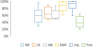

Figure 3.

Percentage of instances predicted as faulty using Alves technique.

To answer RQ2, we notice that the number of instances selected to be added to the minority group (faulty) is increased for all systems using the three threshold techniques as shown in Table 8. Table 8 shows the percentages of faulty instances after using thresholds and their validation using the five machine learning techniques. Therefore, we can conclude that threshold values help reduce data imbalance. To summarize this finding we have reported the boxplots (Figs 2–4) that show the percentages of classes that are selected as fault-prone using thresholds. The use of Shatnawi and Vale thresholds shows that classifiers have selected about 50% of classes as indeed faultprone using the single classifiers as reported in Figs 2 and 4. However, the five classifiers together have selected about 38% of classes as fault-prone. Therefore, we can conclude that RQ2 is answered by the experiment. Threshold values can be used to reduce imbalance in fault data as shown clearly in Table 8. For all systems, Shatnawi’s thresholds reduced data imbalance more than Vales’ and Aleves’ thresholds.

Figure 4.

Percentage of instances predicted as faulty using Vale technique.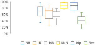

4.3 Fault prediciton with thresholds

Datasets are rebuilt according to the classification of the unlabeled instances. The prediction models are then trained and tested using the 10-fold cross validation on the updated datasets. We report the results of each classifier to compare the updated datasets with the original datasets. The results of the five classifiers are shown in the Tables 9–13. The MCC values of each classifier are shown for the three threshold techniques.

Table 9
NB Classification of faulty and non-faulty

System	Original	Alves	Shatnawi	Vale
Ant	0.02	0.21	0.47	0.54
Camel	0.19	0.46	0.60	0.58
Ivy	0.33	0.50	0.68	0.64
Jedit	0.29	0.45	0.63	0.61
Tomcat	0.24	0.56	0.71	0.72
Prop1	0.27	0.44	0.70	0.58
Prop2	0.09	0.36	0.58	0.67
Prop3	0.21	0.31	0.54	0.54
Prop4	0.21	0.27	0.42	0.37
Prop5	0.20	0.26	0.48	0.44

Table 10

LR Classification of faulty and non-faulty

System	Original	Alves	Shatnawi	Vale
Ant	$-$ 0.07	0.24	0.51	0.56
Camel	0.15	0.50	0.68	0.60
Ivy	0.39	0.57	0.76	0.74
Jedit	0.37	0.48	0.71	0.70
Tomcat	0.28	0.61	0.80	0.80
Prop1	0.22	0.49	0.87	0.69
Prop2	0.06	0.37	0.79	0.76
Prop3	0.13	0.34	0.67	0.61
Prop4	0.22	0.31	0.47	0.40
Prop5	0.20	0.28	0.61	0.45

Table 11

KNN Classification of faulty and non-faulty

System	Original	Alves	Shatnawi	Vale
Ant	$-$ 0.02	0.15	0.45	0.48
Camel	0.17	0.50	0.67	0.61
Ivy	0.24	0.54	0.82	0.76
Jedit	0.26	0.42	0.69	0.67
Tomcat	0.22	0.57	0.80	0.78
Prop1	0.22	0.48	0.88	0.73
Prop2	0.20	0.49	0.93	0.81
Prop3	0.21	0.33	0.72	0.60
Prop4	0.46	0.51	0.64	0.58
Prop5	0.17	0.25	0.69	0.48

The results of classifiers’ performance on the original data are shown in the second column in the Tables 9–13. The classifiers’ performance on the original data (i.e., without the use of thresholds) is weak on all classifiers, i.e. a small MCC value that is close to zero means a random correlation between the actual and the predicted values. The results for the classifiers after using thresholds are also shown in the tables.

Table 12

JRip classification of faulty and non-faulty

System	Original	Alves	Shatnawi	Vale
Ant	0.01	0.28	0.57	0.53
Camel	0.11	0.54	0.70	0.63
Ivy	0.23	0.55	0.71	0.69
Jedit	0.29	0.44	0.76	0.65
Tomcat	0.32	0.62	0.79	0.78
Prop1	0.31	0.52	0.91	0.75
Prop2	0.35	0.54	0.93	0.79
Prop3	0.14	0.31	0.72	0.60
Prop4	0.53	0.58	0.70	0.64
Prop5	0.19	0.30	0.69	0.48

Table 13

C4.5 Classification of faulty and non-faulty

System	Original	Alves	Shatnawi	Vale
Ant	$-$ 0.01	0.29	0.58	0.60
Camel	0.14	0.50	0.70	0.60
Ivy	0.07	0.53	0.71	0.71
Jedit	0.15	0.44	0.79	0.66
Tomcat	0.35	0.57	0.79	0.77
Prop1	0.27	0.51	0.90	0.76
Prop2	0.37	0.53	0.94	0.80
Prop3	0.08	0.31	0.73	0.58
Prop4	0.50	0.57	0.69	0.64
Prop5	0.18	0.27	0.68	0.47

To answer RQ3, we need a more formal analysis to find the significance of the differences between two models, the traditional and the modified models. We conduct a statistical comparison using a non-parametric test, cliff’s $\delta$ test [33]. Cliff’s $\delta$ measures the magnitude of difference between two groups [38]. Cliff’s $\delta$ in this research estimates the likelihood of how often a predictor is becoming better after using thresholds to reduce data imbalance. Song et al have used the following scales: trivial ( $\delta<$ 0.147), small (0.147 $<\delta<$ 0.33), moderate (0.33 $<\delta<$ 0.474) or large ( $\delta>$ 0.474) [38]. We compare the differences in MCC values between the use of each threshold technique and the traditional machine learners. The results of Cliff’s $\delta$ analysis are shown in Table 14. We conclude that the use of thresholds has a large effect on improving the traditional fault-prediction models, i.e., all values are large (i.e., $\delta>$ 0.474). Therefore, this experiment answers RQ3 and provides evidence of using thresholds to improve fault prediction in imbalanced data.

Table 14

Effect size (Cliff’s $\delta$ ) of classifiers with thresholds versus the traditional classifiers

	Alves	Shatnawi	Vale
NB	0.77	1.00	1.00
LR	0.78	1.00	1.00
KNN	0.74	0.98	0.96
Jrip	0.71	1.00	0.97
J48	0.78	1.00	0.98

Figure 5.

Boxplots of classifiers performance (MCC) on ten datasets for (Original, Alves, Shatnawi and Vale).

4.4 Discussion

For comparison purposes, the boxplots for all the classifiers’ performance (MCC values) are reported in Fig. 5. The boxplots show the MCC values for four datasets: original, and modified using Alves, Shatnawi and Vale techniques. The boxplots in Fig. 5 show better prediction performance after using thresholds than otherwise. The performance of using classifiers with Shatnawi and Vale thresholds are better than with Alves thresholds.

For the five classifiers, we observe similar patterns, i.e., the original data has the least performance whereas using Shatnawi thresholds produces the best performance, i.e., the median value is the largest. The MCC values are larger than random in models when using thresholds. These results show reliable prediction models. Generally speaking, using thresholds improves fault prediction performance. The improved classifiers have shown a great improvement on average when compared with models on original data. Table 15 shows the percentage of improvements on the average values of the performance for each model. For example, the performance of models with Shatnawi’s thresholds shows the most improvements for J48 (358%). All thresholds have shown improvements on average. The Alves’ thresholds are showing the least improvement, however, there improvements are significantly large.

Table 15
Improvements on models before and after using thresholds

Models	Alves	Shatnawi	Vale
NB	186%	283%	278%
LR	216%	354%	325%
KNN	199%	342%	305%
Jrip	189%	302%	264%
J48	215%	358%	314%

Threshold values shown in Table 1 can be ordered by the number of instances that are selected for inclusion in faulty classes, i.e., Alves, Vale, and Shatnawi. Shatnawi’s thresholds select more instances for further investigation. Threshold values can be used separately to mark classes as fault-prone or can be used in combination with fault prediction models to improve the prediction performance. This is the reason why Shatnawi’s thresholds have better improvement on the modified datasets than the other threshold techniques. As noticed in Tables 5–7, using thresholds has selected a large number of instances as faulty and we found at least 50% of these instances were classified as such.

Using classifiers such as naïve Bayes, nearest neighbors and JRip show better results than LR and C4.5. However, LR and C4.5 performances were significantly larger than random (MCC $>$ 0). The NB classifiers with Alves’ thresholds show large MCC values between 0.82 and 1. The KNN classifiers with Vale thresholds show large MCC values between 0.75 and 1. The JRip classifiers show values between 0.68 and 0.99. These results suggest that thresholds are reliable to find faulty classes for at least five well-known classifiers. We can conclude that thresholds are reliable in classifying classes as either faulty or non-faulty and the use of thresholds has a consistent effect on different classifiers as shown in the boxplots in Fig. 5.

5. Threats to validity

In this section, we discuss several study limitations:

Internal validity threats: there are static analysis tools that may use variants of metric definitions. For example, the WMC and LCOM metrics have many variants. However, the metrics data in this research are based on the original definitions of C&K metrics. External validity threats: All systems under investigation were developed in Java and the results may not be generalized to other programming languages. Threshold identification techniques and fault prediction models are valid for other languages. Although, there are abundant number of software metrics that have been already proposed, the C&K metrics are the most reported for fault prediction and threshold identification. In addition, the systems under investigation come from two domains only, development tools and insurance business. Construct validity: The fault-proneness variable is defined as binary variable. The number of fault fixes provides more detailed evidence of the software quality. However, most classes are not faulty and therefore, the fault data is sparse and imbalanced. The use of a binary variable is more convenient for analysis. In addition, threshold identification techniques were only reported for binary variables.

6. Conclusions

This research aims to answer three important questions related to the effect of data imbalance on fault-prediction. First, we found data imbalance has a great effect on the performance of fault prediction. Second, thresholds reduced the magnitude of imbalance by increasing the minority instances. Third, the use of thresholds improved the fault prediction significantly when compared with models on the traditional imbalanced data.

In this research, we propose to use thresholds derived from a large benchmark to improve fault-prediction models. Three techniques that were proposed by Shatnawi, Alves and Vale are used in this research. For validation, the datasets of ten object-oriented systems are used. The dataset of each system includes both metric data (C&K suite) and fault data. Data shows imbalance in the ten systems, i.e., the majority of instances are not faulty, whereas the faulty instances are the minority.

Threshold values have identified many instances as faulty. The three threshold identification techniques have increased the number of faulty instances and reduced the imbalance in fault data. However, thresholds may not be accurate in the selection of faulty data. We run five classifiers on the selected instances as testing datasets. If all five classifiers classify an instance as faulty then the instance is marked as such. The process is repeated for all datasets and all three threshold techniques.

The resulting datasets are updated and used to build fault prediction models. The fault prediction models were trained and tested using the 10-cross validation techniques. The results show improvements in the prediction models when compared with the models without the use of thresholds. The performance of using Shatnawi and Vale thresholds have produced models that are better than the ones produced using Alves thresholds.

In conclusion, threshold values can be used as reference points for prioritization and management of software verification and validation efforts. Moreover, threshold values can improve fault-prediction models.

Footnotes

Funding

This work is supported in part by Jordan University of Science and Technology, Deanship of Research.

References

Folleco

Khoshgoftaar

T.M.

Van Hulse

and Bullard

, Software quality modeling: The impact of class noise on the random forest classifier, 2008 IEEE Congress on Evolutionary Computation (IEEE World Congress on Computational Intelligence), Hong Kong, 2008, pp. 3853–3859.

Ghotra

McIntosh

and Hassan

A.E.

, Revisiting the Impact of Classification Techniques on the Performance of Defect Prediction Models, 2015 IEEE/ACM 37th IEEE International Conference on Software Engineering, Florence, 2015, pp. 789–800.

Hailpern

and Santhanam

, Software debugging, testing, and verification, IBM Systems Journal 41(1) (2002), 4–12.

Jiang

Cukic

and Ma

, Techniques for evaluating fault prediction models, Empir Softw Eng 13 (2008), 561–595.

Matthews

, Comparison of the predicted and observed secondary structure of T4 phage lysozyme, Biochimica et Biophysica Acta (BBA) – Protein Structure 405(2) (1975), 442–451.

Catal

Alan

and Balkan

, Class noise detection based on software metrics and ROC curves, Information Sciences 181(21) (2011), 4867–4877.

Seiffert

Khoshgoftaar

T.M.

Van Hulse

and Napolitano

, Building useful models from imbalanced data with sampling and boosting, Proceedings of the Twenty – First International FLAIRS Conference, 2008, pp 206–311.

Aha

Kibler

and Albert

, Instance – based learning algorithms, Machine Learning 6(1) (1991), 37–66.

Gray

Bowes

Davey

Sun

and Christianson

, The misuse of the NASA metrics data program data sets for automated software defect prediction, in Evaluation and Assessment in Software Engineering (EASE), 2011.

10.

Powers

, Evaluation: From precision, recall and f-measure to roc, informedness, markedness & correlation, Journal of Machine Learning Technologies 2(1) (2011), 37–63.

11.

Tempero

et al., The Qualitas Corpus: A Curated Collection of Java Code for Empirical Studies, 2010 Asia Pacific Software Engineering Conference, Sydney, NSW, 2010, pp. 336–345.

12.

Zhang

Mockus

Keivanloo

and Zou

, Towards building a universal defect prediction model with rank transformed predictors, Empir Software Eng 2(5) (2016), 2107–2145.

13.

John

and Langley

, Estimating continuous distributions in Bayesian classifiers, in: Proceedings of the Eleventh Conference on Uncertainty in Artificial Intelligence, in: Besnard

and Hanks

, eds, San Francisco, CA: Morgan Kaufmann, 1995, pp. 338–345.

14.

Vale

Fernandes

and Figueiredo

, On the proposal and evaluation of a benchmark-based threshold derivation method, Software Quality Journal 27(1) (2018), 1–32.

15.

and Garcia

, Learning from imbalanced data, IEEE Transactions on Knowledge and Data Engineering 21(9) (2009), 1264–1284.

16.

Al Dallal

, The impact of accounting for special methods in the measurement of object-oriented class cohesion on refactoring and fault prediction activities, The Journal of Systems and Software 85(5) (2012), 1042–1057.

17.

Sáez

Galar

Luengo

and Herrera

, Tackling the problem of classification with noisy data using Multiple Classifier Systems: Analysis of the performance and robustness, Information Sciences 247 (2013), pp. 1–20.

18.

Van Hulse

and Khoshgoftaar

, Knowledge discovery from imbalanced and noisy data, Data and Knowledge Engineering 68(12) (2009), 1513–1542.

19.

Quinlan

J.R.

, C4.5: Programs for machine learning, Morgan Kaufmann Publishers, San Mateo, 1993.

20.

Ferreira

Bigonha

Mendes

and Almeida

, Identifying thresholds for object – oriented software metrics, The Journal of Systems and Software 85(2) (2012), 244–257.

21.

Gao

Khoshgoftaar

T.M.

and Seliya

, Predicting high-risk program classes by selecting the right software measurements, Software Quality Journal 20 (2012), 3–42.

22.

Khomh

and Gueheneuc

, An empirical study of crash-inducing commits in Mozilla Firefox, Software Quality Journal 26(2) (2018), 553–584.

23.

Basili

Briand

and Melo

, A validation of object–oriented design metrics as quality indicators, IEEE Transactions on Software Engineering 22(1) (1996), 751–761.

24.

Briand

Wüst

and Lounis

, Replicated case studies for investigating quality factors in object–oriented designs, Empirical Software Engineering 6(1) (2001), 11–58.

25.

Briand

L.C.

Wüst

Daly

and Porter

, Exploring the relationship between design measures and software quality in object-oriented systems, J Syst Softw 51(3) (2000), 245–273.

26.

Hamill

and Goseva-Popstojanova

, Exploring the missing link: An empirical study of software fixes, Software Testing, Verification and Reliability 24(5) (2014), 49–71.

27.

Jureczko

and Spinellis

, Using object-oriented design metrics to predict software defects, In: Proceedings of the 5th International Conference on Dependability of Computer Systems, 2010, pp. 69–81.

28.

Jureczko

and Madeyski

, Towards identifying software project clusters with regard to defect prediction, In Proceedings of the 6th International Conference on Predictive Models in Software Engineering, 2010, pp. 1–10.

29.

Kubat

and Matwin

, Addressing the curse of imbalanced training sets: one–sided selection, Proceedings of the Fourteenth International Conference on Machine Learning, 1997, pp. 179–186.

30.

Lorenz

and Kidd

, Object-oriented Software Metrics, Prentice-Hall: Englewood Cliffs NJ, 1994.

31.

Shepperd

Bowes

and Hall

, Researcher Bias: The Use of Machine Learning in Software Defect Prediction, IEEE Transactions on Software Engineering 40(6) (2014), 603–616.

32.

Chawla

, C4.5 and Imbalanced Data sets: Investigating the effect of sampling method, probabilistic estimate, and decision tree structure, Workshop on Learning from Imbalanced Datasets II, ICML, 2003, Washington DC.

33.

Cliff

, Dominance statistics: Ordinal analyses to answer ordinal questions, Psychological Bulletin 114(3) (1993), 494–509.

34.

Arar

Ö.F.

and Ayan

, Software defect prediction using cost-sensitive neural network, Applied Soft Computing 33 (2015), 263–277.

35.

Liu

Chen

and Ma

, An empirical study on software defect prediction with a simplified metric set, Information and Software Technology 59 (2015), 170–190.

36.

Oliveira

Valente

M.T.

and Lima

F.P.

, Extracting relative thresholds for source code metrics, Software Evolution Week – IEEE Conference on Software Maintenance, Reengineering, and Reverse Engineering (CSMR-WCRE), Antwerp, 2014, pp. 254–263.

37.

Singh

and Verma

, ACO based comprehensive model for software fault prediction, 24(1) (2020), 63–71.

38.

Song

Guo

and Shepperd

, A comprehensive investigation of the role of imbalanced learning for software defect prediction, IEEE Transactions on Software Engineering 45(12) (2019), 1253–1269.

39.

Malhotra

and Bansal

, Fault prediction considering threshold effects of object-oriented metrics, Expert Systems 32 (2015), 203–219.

40.

Shatnawi

and Li

, The effectiveness of software metrics in identifying error-prone classes in post-release software evolution process, Journal of Systems and Software 81(11) (2008), 1868–1882.

41.

Shatnawi

, Deriving metrics thresholds using log transformation, J Softw Evol and Proc 27 (2015), 95–113.

42.

Shatnawi

, Quantitative investigation of the acceptable risk levels of object – oriented metrics in open – source systems, IEEE Trans Software Eng 36(2) (2010), 216–225.

43.

Shatnawi

Swain

and Newman

, Finding software metrics threshold values using ROC curves, Journal of Software Maintenance & Evolution, Research & Practice 22(1) (2010), 1–16.

44.

Benlarbi

El Emam

Goel

and Rai

, Thresholds for object-oriented measures, Proceedings 11th International Symposium on Software Reliability Engineering, ISSRE 2000, San Jose, CA, USA, 2000, pp. 24–38.

45.

Chidamber

and Kemerer

, A metrics suite for object oriented design, IEEE Trans Software Eng 20(6) (1994), 476–493.

46.

Lessmann

Baesens

Mues

and Pietsch

, Benchmarking classification models for software defect prediction: a proposed framework and novel findings, IEEE Transactions on Software Engineering 34(4) (July-Aug. 2008), 485–496.

47.

Shukla

Radhakrishnan

Muthukumaran

Neti

, Multi-objective cross-version defect prediction, Soft Comput 22(6) (2018), pp. 1959–1980.

48.

Wang

and Yao

, Using class imbalance learning for software defect prediction, IEEE Transactions on Reliability 62(2) (2013), 434–443.

49.

Rathore

S.S.

and Kumar

, Towards an ensemble based system for predicting the number of software faults, Expert Syst Appl 82 (2017), 357–382.

50.

Alves

Ypma

and Visser

, Deriving metric thresholds from benchmark data, 2010 IEEE International Conference on Software Maintenance, 2010, pp. 1–10.

51.

Fukushima

Kamei

McIntosh

Yamashita

and Ubayashi

, An empirical study of just-in-time defect prediction using cross-project models, In Proceedings of the 11th Working Conference on Mining Software Repositories, 2014, pp. 172–181.

52.

Menzies

Greenwald

and Frank

, Data mining static code attributes to learn defect predictors, IEEE Transactions on Software Engineering 33(1) (2007), 2–13.

53.

Cohen

, Fast effective rule induction, In: Twelfth International Conference on Machine Learning, 1995, pp. 115–123.

54.

, Another metric suite for object oriented programming, The Journal of Systems and Software 44(2) (1998), 155–162.

Software fault prediction using machine learning techniques with metric thresholds

Abstract

BACKGROUND:

AIM:

METHOD:

RESULTS:

CONCLUSION:

Keywords

1. Introduction

2.1 Fault prediction in literature

2.2 Fault data quality

2.3 Thresholds techniques

3. Methodology

Table 2 Thresholds used in this research

3.4 Machine learning techniques

Table 3 The confusion matrix of classification models

4.1 Traditional fault-prediction models

4.2 Data imbalance effect

Table 5 Number of unlabeled instances selected fault-prone using Shatnawi thresholds

Table 9 NB Classification of faulty and non-faulty

Table 15 Improvements on models before and after using thresholds

6. Conclusions

Footnotes

Funding

References

Table 2
Thresholds used in this research

Table 3
The confusion matrix of classification models

Table 5
Number of unlabeled instances selected fault-prone using Shatnawi thresholds

Table 9
NB Classification of faulty and non-faulty

Table 15
Improvements on models before and after using thresholds