Weighted power mean copulas: theory and application

Abstract

It is well known that the arithmetic mean of two possibly different copulas forms a copula, again. More generally, we focus on the weighted power mean (WPM) of two arbitrary copulas which is not necessary a copula again, as different counterexamples reveal. However, various conditions regarding the mean function and the underlying copula are given which guarantee that a proper copula (so-called WPM copula) results. In this case, we also derive dependence properties of WPM copulas and give some brief application to financial return series.

Keywords

Copulas generalized power mean max id left tail decreasing tail dependence

1. Introduction

For two given copulas $C_{1}(u,v)$ and $C_{2}(u,v)$ we consider the function

$\overline{C}_{r}(u,v)\equiv\Big{(}\alpha C_{1}(u,v)^{r}+(1-\alpha)C_{2}(u,v)^{% r}\Big{)}^{1/r}$ (1)

on $[0,1]\times[0,1]$ , where $r\in\mathbb{R}$ and $\alpha\in(0,1)$ . Letting $r\rightarrow 0$ , Eq. (1) reduces to the weighted geometric mean of $C_{1}$ and $C_{2}$ ,

$\overline{C}_{0}(u,v)=C_{1}(u,v)^{\alpha}C_{2}(u,v)^{1-\alpha}.$ (2)

Assuming that $\overline{C}_{r}(u,v)$ is again a copula – which is not guaranteed at all – it is governed by – beside of the specific copula parameters of $C_{1}$ and $C_{2}$ – by two additional parameters $r$ and $\alpha$ which may allow for more flexibility regarding dependence modelling. In this case, $\overline{C}_{r}$ will be denoted as weighted power mean copula, or briefly WPM copula.

Certainly, there are single results on weighted arithmetic, geometric or harmonic means of two specific copulas (see, e.g. Nelsen, 2006; Fischer & Dörflinger, 2010). Nelsen even shows, that certain copula families are closed with respect to the operation in Eq. (1), i.e. $\overline{C}_{r}$ belongs to the same copula family as $C_{1}$ and $C_{2}$ for a fixed $r$ . But a systematic proof that $\overline{C}_{r}$ is a copula for all $r$ can only be found for the weighted power mean of the maximum- and independence copulas (see Fischer & Hinzmann, 2014).

On the other hand, we will provide counterexamples within this paper, where the weighted power mean of two copulas fails to satisfy the postulates of the copula definition. This motivates the derivation of certain criteria for $C_{1}$ and $C_{2}$ such that $\overline{C}_{r}$ is again a copula. Therefore, our objective is to give solutions for broad classes of copulas $C_{1}$ and $C_{2}$ and possibly comprehensive domain of $r$ .

For this reason, the paper is organized as follows: First of all, we restrict ourselves to benign copulas $C_{1}$ and $C_{2}$ , where the copula densities exist and, consequently, the two-increasing condition is valid if $\frac{\partial^{2}\overline{C}_{r}}{\partial u\partial v}$ is non-negative. Up to a few special cases (see, for instance, Fischer & Hinzmann, 2014), the direct proof of the two increasing-condition seems to be impossible without assuming the existence of the density. We then show that this sufficient (but not necessary) condition is satisfied for extrem value copulas and positive $r$ . Applying weighted power means with positive $r$ to max-id copulas will also result in proper copulas. As the max-id property of Archimedean copulas can be easily checked, we will provide results for various Archimedean copulas. It will also be shown that combining a copula with a specific positive dependence structure (i.e. left-tail decreasing property) with the independence copula gives again a copula. For $r<0$ , we are only able to derive single results for specific copulas. Afterwards, we investigate how the dependence structure of $C_{1}$ and $C_{2}$ transforms to the WPM-copula. For the positive quadrant ordering of Lehmann, 1966 and the stronger positive ordering of Colangelo, 2006, which is based on the concept of tail dependence (so-called LTD-ordering) it will be shown that the WPM-copula (with respect to these orderings) measures a strength/degree of positive ordering which lies between those of $C_{1}$ and $C_{2}$ . This implies that well-known dependence measures like Spearman’s $\rho$ and Kendall’s $\tau$ (which both satisfy these orderings) of WPM-copulas lie also in between those of $C_{1}$ and $C_{2}$ . However, only numerical approximation to these measures are available because no closed formula can be derived in general. After that, general formulas for the weak and strong tail dependence coefficients of WPM copulas are derived. Finally, we discuss the joint estimation of the WPM parameters $r$ and $\alpha$ together with the copula parameters of $C_{1}$ and $C_{2}$ and apply the estimation formula to empirical data.

The following Table 1 summarizes the results of this contribution.

Table 1

Summary of the results

Theorem 1	Eq. (8) holds	Eq. (8) holds	$r\geqslant 1$ and Eq. (8) holds
	$C_{1}$	$C_{2}$	$\overline{C}_{r}$ is a copula if
Theorem 2	EV copula	EV copula	$r>0$
Theorem 3	Max-id	Max-id	$r\in[0,1)$
Theorem 4	LTD	Indep. copula	$r\geqslant 1$
Theorem 5	Result on LTD-property of $\overline{C}_{r}$
Theorem 6	Result on strong TDC of $\overline{C}_{r}$
Theorem 7	Result on weak TDC of $\overline{C}_{r}$

2. A short primer on copulas

Let $[a,b]\subseteq\mathbb{R}$ . A function $K:[a,b]\times[a,b]\rightarrow\mathbb{R}$ is said to be $2$ -increasing if its $K$ -volume

$V_{K}(u_{1},u_{2},v_{1},v_{2})\equiv K(u_{2},v_{2})-K(u_{2},v_{1})-K(u_{1},v_{% 2})+K(u_{1},v_{1})\geqslant 0$ (3)

for all $a\leqslant u_{1}\leqslant u_{2}\leqslant b$ and $a\leqslant v_{1}\leqslant v_{2}\leqslant b$ . If, additionally, $[a,b]=[0,1]$ and $K$ satisfies the boundary conditions

$K(u,0)=K(0,v)=0,\quad K(u,1)=u\,\,\text{and }\,\,K(1,v)=v$ (4)

for arbitrary $u,v\in[0,1]$ , $K$ is commonly termed as copula and we write $C$ , instead.

Putting a different way, let $X$ and $Y$ denote two random variables with joint distribution $F_{X,Y}(x,y)$ and continuous marginal distribution functions $F_{X}(x)$ and $F_{Y}(y)$ . According to Sklar’s Sklar, 1959 fundamental theorem, there exists a unique decomposition

$\displaystyle F_{X,Y}(x,y)=C(F_{X}(x),F_{Y}(y))$

of the joint distribution into its marginal distribution functions and the so-called copula

$C(u,v)=P(U\leqslant u,V\leqslant v),\quad U\equiv F_{X}(X),\quad V\equiv F_{Y}% (Y)$ (5)

on $[0,1]^{2}$ which comprises the information about the underlying dependence structure. From Eq. (5) it becomes obvious that a copula is a bivariate distribution function of a pair of random variable $(U,V)$ defined on $[0,1]\times[0,1]$ . Assuming that $C$ is differentiable with respect to both arguments, Eq. (3) is satisfied if

$\displaystyle c(u,v)\equiv\frac{\partial^{2}C(u,v)}{\partial u\partial v}% \geqslant 0.$

Moreover, it is known that

$\frac{\partial C(u,v)}{\partial u}=P(V\leqslant v|U=u)\geqslant 0\,\,\text{and% }\,\,\frac{\partial C(u,v)}{\partial v}=P(V\leqslant v|U=u)\geqslant 0.$ (6)

Later on, we will frequently use the independence copula $C_{I}(u,v)=uv$ which corresponds to bivariate distributions with independent marginals, the maximum copula $C_{U}(u,v)=\min\{u,v\}$ , associated to random variables which are co-monotone and, thus, constituting an upper bound for all copulas and the minimum copula $C_{U}(u,v)=\max\{u+v-1,0\}$ , associated to random variables which are counter-monotone and, thus, constituting a lower bound for all copulas. A copula which comprises minimum, maximum and independence copula is commonly called comprehensive.

For a general introduction to copulas we refer to Nelsen (2006) or Joe (1997). A recent overview on the multivariate case is provided by Fischer (2010) or Fischer and Köck (2012). Applications to finance are given, for instance, by Fischer et al. (2009).

3. Examples and counterexamples

In the literature there are numerous examples of copulas which are specific means of other copulas. Joe (1997), for instance, considers copula B11

$\displaystyle C(u,v)=\alpha\min(u,v)+(1-\alpha)uv$

which composes as weighted arithmetic mean of the maximum copula and of the independence copula. Similarly, copula B12 in Joe (1997)

$\displaystyle C(u,v)=\min(u,v)^{\alpha}(uv)^{1-\alpha}\;\;\alpha\in[0,1]$

results as the corresponding geometric mean of both copulas. Nelsen (2006) investigates whether the mean of two copulas with a specific building law is again a copula with the same building law. Consider, for example, the weighted arithmetic mean of two Farlie-Gumbel-Morgenstern copulas with the building law

$\displaystyle C_{i}(u,v)=uv+\theta_{i}uv(1-u)(1-v),\;\;\theta_{i}\in[-1,1],\;i% =1,2,$

which results again in a Farlie-Gumbel-Morgenstern copula:

$\displaystyle\alpha C_{1}(u,v)+(1-\alpha)C_{2}(u,v)=uv+(\alpha\theta_{1}+(1-% \alpha)\theta_{2})u(1-u)v(1-v).$

A similar result is proven by Nelsen (2006, p. 107) for weighted geometric means and Gumbel-Barnett copulas which are defined by

$\displaystyle C_{i}(u,v)=uv\exp(-\theta_{i}\ln u\ln v),\;\;\theta_{i}\in(0,1],% \;i=1,2.$

Consequently, the geometric mean of $C_{1}$ and $C_{2}$ ,

$\displaystyle C_{1}(u,v)^{\alpha}C_{2}(u,v)^{1-\alpha}=uv\exp(-(\alpha\theta_{% 1}+(1-\alpha)\theta_{2})\ln u\ln v)$

is again a Gumbel-Barnett copula. Also the weighted harmonic mean can be successfully used to construct new copulas. Starting from Ali-Mikhail-Haq copulas (see Nelsen, 2006, p. 82) of the form

$\displaystyle C_{i}(u,v)=\frac{uv}{1-\theta_{i}(1-u)(1-v)},\;\theta_{i}\in[-1,% 1],\;\;i=1,2,$

the weighted harmonic mean

$\displaystyle\left(\alpha\frac{1}{C_{1}(u,v)}+(1-\alpha)\frac{1}{C_{2}(u,v)}% \right)^{-1}=\frac{uv}{1-(\alpha\theta_{1}+(1-\alpha)\theta_{2})(1-u)(1-v)}$

is again a Ali-Mikhail-Haq copula. Fischer and Hinzmann (2014) turn away from concrete means and consider the broad class of so-called power means which are of the form

$\displaystyle\overline{C}_{r}(u,v)=\left(\alpha\min(u,v)^{r}+(1-\alpha)(uv)^{r% }\right)^{1/r},\;\;\alpha\in[0,1]$

where $r\in\mathbb{R}$ . Included as special and limiting cases are the weighted arithmetic ( $r=1$ , B11), the weighted geometric ( $r\rightarrow 0$ , B12) and the weighted harmonic mean ( $r=-1$ ). Fischer and Hinzmann (2014) proved that $\overline{C}_{r}(u,v)$ is again a copula for all $r\in\mathbb{R}$ . Due to the simple structure of both copulas, the authors succeed in verifying the $2$ -increasing-condition even without using the copula density.

In contrast, the question whether in general the weighted power mean of two copulas is again a copula has to be negotiated. Consider, for instance, the following simple counterexamples:

(Counterexamples).

1. Given the specific power mean of the minimum and the maximum copula, i.e

$\displaystyle K(u,v)=\left(\alpha(uv)^{r}+(1-a)\max\{u+v-1,0\}^{r}\right)^{1/r}$

with $\alpha=0.5$ and $r=-1$ (harmonic mean). Plugging $u_{1}=0.6564$ , $u_{2}=0.9114$ , $v_{1}=0.3450$ and $v_{2}=0.9240$ into the formula above,

$\displaystyle K(u_{2},v_{2})=0.8388,\;K(u_{2},v_{1})=0.2825,\;K(u_{1},v_{2})=0% .5932,\;K(u_{1},v_{1})=0.0028.$

Hence, $K(u_{2},v_{2})-K(u_{1},v_{2})-K(u_{2},v_{1})+K(u_{1},v_{1})=-0.0341<0$ and the $2$ -increasing condition is no longer valid, i.e. $K(u,v)$ is no copula.

2. Consider $K(x,y)=\left(0.5\sqrt{C_{I}(x,y)}+0.5\sqrt{C_{L}(x,y)}\right)^{2}$ , where $C_{I}$ denotes the independence copula and $C_{L}$ the minimum copula. It can be checked that the $K$ -volume of $[0.8,0.9]\times[0.2,0.3]$ is negative: $K(0.9,0.3)=0.2336895$ , $K(0.8,0.3)=0.1624597$ , $K(0.9,0.2)=0.1370820$ , $K(0.8,0.2)=0.04$ and hence

$V_{K}(0.9,0.8,0.3,0.2)=0.2336895-0.1624597-0.1370820+0.04\approx-0.0258522<0.$

4. Sufficient conditions

Obviously, the boundary conditions of a copula are easily checked for the weighted power mean of two given copulas:

$\displaystyle C(u,1)=\left(\alpha C_{1}(u,1)^{r}+(1-\alpha)C_{2}(u,1)^{r}% \right)^{1/r}=\left(\alpha u^{r}+(1-\alpha)u^{r}\right)^{1^{/}r}=u$

for $0<u<1$ . The crucial point is the proof of the $2$ -increasing condition. If we focus on copulas with existing densities, it suffices to show that the second mixed derivative of $C$ is non-negative. In the general case of WPM copula the mixed derivative of $C$ is given by

$\displaystyle\frac{\partial^{2}}{\partial u\partial v}\overline{C}_{r}(u,v)=% \frac{\partial^{2}}{\partial u\partial v}\left(\alpha C_{1}(u,v)^{r}+(1-\alpha% )C_{2}(u,v)^{r}\right)^{1/r}==\frac{1}{r}\frac{M^{1/r}}{M^{2}}\left(\frac{1-r}% {r}AB+MC\right),$ (7)

where $M\equiv\alpha C_{1}(u,v)^{r}+(1-\alpha)C_{2}(u,v)^{r}\geqslant 0$ ,

$\displaystyle A=\alpha\frac{\partial}{\partial v}C_{1}(u,v)^{r}+(1-\alpha)% \frac{\partial}{\partial v}C_{2}(u,v)^{r},\,\,B=\alpha\frac{\partial}{\partial u% }C_{1}(u,v)^{r}+(1-\alpha)\frac{\partial}{\partial u}C_{2}(u,v)^{r},$ $\displaystyle C=\alpha\frac{\partial^{2}}{\partial u\partial v}C_{1}(u,v)^{r}+% (1-\alpha)\frac{\partial^{2}}{\partial u\partial v}C_{2}(u,v)^{r}.$

Whether $A$ , $B$ and $C$ are non-negative depends in particular on the sign and amount of $r$ . For $r\geqslant 1$ it immediately follows that both $A$ , $B$ (according to Eq. (6)) and $C$ (due the existence of the copula density of $C_{i}$ , $i=1,2$ ) are non-negative. On the other hand, the sign of $(1-r)/rAB$ is non-positive for $r\geqslant 1$ . However, using the equivalent representation

$\displaystyle\frac{1}{K}\frac{\partial^{2}\overline{C}_{r}}{\partial u\partial v% }=\alpha^{2}\frac{c_{1}}{C_{1}}\left(\frac{C_{1}}{C_{2}}\right)^{r}+\alpha(1-% \alpha)\frac{c_{1}}{C_{1}}+\alpha(1-\alpha)\frac{c_{2}}{C_{2}}+(1-\alpha)^{2}% \frac{c_{2}}{C_{2}}\left(\frac{C_{2}}{C_{1}}\right)^{r}-(1-r)\alpha(1-\alpha)% \left(\frac{\partial\ln C_{1}}{\partial u}-\frac{\partial\ln C_{2}}{\partial u% }\right)\left(\frac{\partial\ln C_{1}}{\partial v}-\frac{\partial\ln C_{2}}{% \partial v}\right)$ (8)

with

$\displaystyle K=\frac{\overline{C}_{r}(u,v)}{(\alpha C_{1}(u,v)^{r}+(1-\alpha)% C_{2}(u,v)^{r})^{2}}C_{1}(u,v)^{r}C_{2}(u,v)^{r}>0$

and where $c_{i}$ denotes the copula density of $C_{i}$ for $i=1,2$ , we derive the sufficient condition

$\left(\frac{\partial\ln C_{1}}{\partial u}-\frac{\partial\ln C_{2}}{\partial u% }\right)\left(\frac{\partial\ln C_{1}}{\partial v}-\frac{\partial\ln C_{2}}{% \partial v}\right)\geqslant 0$ (9)

that $\overline{C}_{r}$ is a copula for all $r\geqslant 1$ . In toto, we proved a very general result for $r\geqslant 1$ :

.

For two copulas $C_{1}$ , $C_{2}$ with Eq. (9) the weighted power mean of $C_{1}$ and $C_{2}$ is again a copula for all $r\geqslant 1$ .

Remark: The construction in Eq. (1) is actually a special type of ”pointwise composition of copulas” in Durante (2009). In particular, by using Theorem $2$ in Durante (2009) with $f_{1}$ , $f_{2}$ , $g_{1}$ , $g_{2}$ equal to the identity function, the prove of Theorem $1$ above can be done without any assumption on the densities of the copulas $C_{1}$ , $C_{2}$ .

.

Consider two Gumbel-Barnett copulas with different parameters $\theta_{1},\theta_{2}$ . For $C_{i}(u,v)=uv\exp$ $\left(\theta_{i}\ln u\ln v\right)$ ,

$\frac{\partial\ln C_{i}(u,v)}{\partial u}=\frac{1}{u}-\theta_{i}\frac{\ln v}{u% },\quad\frac{\partial\ln C_{1}(u,v)}{\partial u}-\frac{\partial\ln C_{2}(u,v)}% {\partial u}=\left(\theta_{2}-\theta_{1}\right)\frac{\ln v}{u}.$ (10)

Hence, the expression in brackets in Eq. (10) are positive for $\theta_{1}>\theta_{2}$ and negative for $\theta_{1}<\theta_{2}$ . In both cases, the condition from above is satisfied.

Remark: In case of $0<r<1$ , $A$ and $B$ and hence $(1-r)/rAB$ are non-negative; the term $C$ may be also negative if the first expression (summand) is negative. For $r<0$ , $A$ and $B$ are non-positive and, consequently, $(1-r)/rAB$ not non-negative. The sign of $C$ is again undetermined, because $r(r-1)>0$ . To sum up, for $r<1$ we obtain no general result for copulas $C_{i}$ , $i=1,2$ . Additional requirements have to be put on $C_{i}$ , $i=1,2$ to obtain a specific result.

Remark: Finally, let’s consider the special case of the weighted geometric mean which results for $r\rightarrow 0$ . For

$\displaystyle\overline{C}_{0}(u,v)=C_{1}(u,v)^{\alpha}C_{2}(u,v)^{1-\alpha}=% \exp\left(\alpha\ln C_{1}(u,v)+(1-\alpha)\ln C_{2}(u,v)\right)$ (11)

we derive that

$\displaystyle\frac{\partial^{2}}{\partial u\partial v}\exp\left(\alpha\ln C_{1% }(u,v)+(1-\alpha)\ln C_{2}(u,v)\right)=C(u,v;r=0,\alpha)(DE+F),$ (12)

where

$\displaystyle D=\alpha\frac{\frac{\partial C_{1}(u,v)}{\partial u}}{C_{1}(u,v)% }+(1-\alpha)\frac{\frac{\partial C_{2}(u,v)}{\partial u}}{C_{2}(u,v)}\geqslant 0% ,\quad E=\alpha\frac{\frac{\partial C_{1}(u,v)}{\partial v}}{C_{1}(u,v)}+(1-% \alpha)\frac{\frac{\partial C_{2}(u,v)}{\partial v}}{C_{2}(u,v)}\geqslant 0$

and

$\displaystyle F=\alpha\frac{C_{1}(u,v)c_{1}(u,v)-\frac{\partial}{\partial v}C_% {1}(u,v)\frac{\partial}{\partial u}C_{1}(u,v)}{C_{1}(u,v)^{2}}+(1-\alpha)\frac% {C_{2}(u,v)c_{2}(u,v)-\frac{\partial}{\partial v}C_{2}(u,v)\frac{\partial}{% \partial u}C_{2}(u,v)}{C_{2}(u,v)^{2}}.$ (13)

However, the sign of the expression $F$ is undetermined.

5. Results for specific copula classes

5.1 Extreme-value copulas

Consider now the first restriction that $C_{i}$ , $i=1,2$ are extreme-value copulas. In this case $C_{i}^{r}(u,v)=C_{i}(u^{r},v^{r})$ for $r>0$ and $i=1,2$ . For expression $C$ we obtain

$\displaystyle\frac{\partial^{2}}{\partial u\partial v}C_{i}^{r}(u,v)=\frac{% \partial^{2}}{\partial u^{r}\partial v^{r}}C_{i}(u^{r},v^{r})\frac{\partial}{% \partial v}v^{r}\frac{\partial}{\partial u}u^{r}\geqslant 0,$

such that $AB+MC\geqslant 0$ holds and we can state the following theorem.

.

The weighted power mean $\overline{C}_{r}(u,v)$ of two arbitrary extreme-value copulas $C_{1}(u,v)$ and $C_{2}(u,v)$ is again a copula for $r\in(0,1)$ .

(WPM-logistic).

Assume that $r>0$ and $\alpha\in[0,1]$ . Combining two possibly different logistic extreme-value copulas by means of a weighted power mean function, the resulting four-parameter copula has the form

$\displaystyle C(u,v;\theta)=\left[\alpha\exp{\left[\widetilde{u}^{1/\lambda_{1% }}+\widetilde{v}^{1/\lambda_{1}}\right]^{r\lambda_{1}}}+(1-\alpha)\exp{\left[% \widetilde{u}^{1/\lambda_{2}}+\widetilde{v}^{1/\lambda_{2}}\right]^{r\lambda_{% 2}}}\right]^{1/r}$

with

$\displaystyle\widetilde{u}=-\ln(u),\theta\equiv(\alpha,r,\lambda_{1},\lambda_{% 2})\ \text{and}\ 0<\lambda_{1},\lambda_{2}\leqslant 1.$

5.2 Max-id copulas

Instead of restricting to extreme-value copulas, we extend our analysis to copulas which are maximal infinitely divisible (max-id). Originally, the max-id property for distribution functions is intensively discussed by Joe (1997). As copulas can be simply extended to distribution functions, we can apply the max-id property direct to copulas. A copula $C(u,v)$ will be denoted as max-id, if $C(u,v)^{m}$ satisfies the properties of a bivariate distribution function for all $m>0$ . Note that $C^{m}$ is not a copula for $m\neq 1$ because the boundary conditions are no longer valid. Consider a bivariate copula $C$ with copula density $c$ . In order to be max-id it has to be shown that

$\frac{\partial^{2}C(u,v)^{m}}{\partial u\partial v}=mC^{m-2}\left(Cc+(m-1)% \frac{\partial C}{\partial u}\frac{\partial C}{\partial v}\right)\geqslant 0% \quad\forall\,(u,v)\in[0,1]\times[0,1].$ (14)

Replacing $C$ by $\overline{C}_{r}$ in Eq. (14) and after some re-arrangement we obtain

$\displaystyle\frac{1}{K}\frac{\partial^{2}\overline{C}_{r}(u,v)}{\partial u% \partial v}=\alpha^{2}\frac{c_{1}}{C_{1}}\left(\frac{C_{1}}{C_{2}}\right)^{r}+% (1-\alpha)^{2}\frac{c_{2}}{C_{2}}\left(\frac{C_{2}}{C_{1}}\right)^{r}+(1-r)% \alpha(1-\alpha)\frac{\partial\ln C_{1}}{\partial v}\frac{\partial\ln C_{2}}{% \partial u}+(1-r)\alpha(1-\alpha)\frac{\partial\ln C_{1}}{\partial u}\frac{% \partial\ln C_{2}}{\partial v}+\alpha(1-\alpha)\frac{1}{C_{1}^{2}}\left(C_{1}c% _{1}-(1-r)\frac{\partial C_{1}}{\partial u}\frac{\partial C_{1}}{\partial v}% \right)+\alpha(1-\alpha)\frac{1}{C_{2}^{2}}\left(C_{2}c_{2}-(1-r)\frac{% \partial C_{2}}{\partial u}\frac{\partial C_{2}}{\partial v}\right)$

$\displaystyle\text{ for}K\equiv\frac{\overline{C}_{r}}{(\alpha C_{1}^{r}+(1-% \alpha)C_{2}^{r})^{2}}C_{1}^{r}C_{2}^{r}>0.$

This expression is positive, if $C_{1}$ and $C_{2}$ satisfy condition Eq. (14), i.e. are both max-id. Obviously, this assertion also holds for $r=0$ , because $D,E\geqslant 0$ and if $C_{1},C_{2}$ are both max-id we obtain $F\geqslant 0$ , notation as in Eq. (13). Hence, we derived the following result:

.

Assume that $C_{1}(u,v)$ and $C_{2}(u,v)$ are two max-id copulas and $r\in[0,1)$ . Then $\overline{C}_{r}$ is again a copula.

We conclude with two examples of max-id copulas.

.

The logarithm of the Galambos copula with parameter $\delta\in(0,\infty)$ is given by

$\displaystyle\ln C_{\delta}=\ln u+\ln v+\left((-\ln u)^{-\delta}+(-\ln u)^{-% \delta}\right)^{-1/\delta}$

and hence

$\displaystyle\frac{\partial^{2}\ln C_{\delta}}{\partial u\partial v}=(a+\delta% )\left((-\ln u)^{-\delta}+(-\ln v)^{-\delta}\right)^{-(s\delta+2)/\delta}\left% ((-\ln u)(-\ln v)\right)^{-\delta-1}\geqslant 0.$

.

Taking the logarithm of the FGM-Copula $C_{\theta}(u,v)=uv(1+\theta(1-u)(1-v))$ with parameter $\theta\in[-1,1]$ ,

$\displaystyle\ln C_{\theta}(u,v)=\ln u+\ln v+\ln\left(1+\theta(1-u)(1-v)\right).$

The corresponding derivatives are given by

$\frac{\partial^{2}\ln C_{\theta}(u,v)}{\partial u\partial v}=\frac{\theta}{% \left(1+\theta(1-u)(1-v)\right)^{2}},$ (15)

which means that the max-id property depends only upon the sign of the parameter.

In particular, Archimedean copula $C_{\phi}$ with continuous, convex and strictly monotone decreasing generators $\phi$ – which guarantees that the inverse function $\phi^{-1}$ exists – are max-id if and only if $-\ln\phi^{-1}\in\mathcal{L}_{2}^{*},$ where

$\displaystyle\mathcal{L}_{2}^{*}\equiv\{\omega:[0,\infty]\rightarrow[0,\infty]% ,\omega(\infty)=\infty,\mbox{sign}(\omega^{(i)})\neq(-1)^{i},i=1,2\}.$

The following table summarizes Archimedean copulas for which the max-id property has already been verified (Nikoloulopoulos & Karlis, 2010) and own calculations), the names and equations are adopted from Nelsen (2006).

Table 2

Selected Archimedean max-id copulas

Name	Copula function	Parameter
Clayton	$\left(u^{-\theta}+v^{-\theta}-1\right)^{-1/\theta}$	$\theta>0$
AMH	${uv}/({1-\theta(1-u)(1-v)})$	$\theta\geqslant 0$
Gumbel	$\exp\left(-\left((-\ln u)^{\theta}+(-\ln v)^{\theta}\right)^{{1}/{\theta}}\right)$	$\theta\geqslant 1$
Frank	$-\theta^{-1}\ln\left(1+{(\exp({-\theta u})-1)(\exp({-\theta v})-1)}/(\exp(-% \theta)-1))\right)$	$\theta>0$
Joe	$1-\left((1-u)^{\theta}+(1-v)^{\theta}+(1-u)^{\theta}(1-v)^{\theta}\right)^{{1}% /{\theta}}$	$\theta\geqslant 1$
( $4.2.12$ )	$\left(1+\left((u^{-1}-1)^{\theta}+(v^{-1}-1)^{\theta}\right)^{{1}/{\theta}}% \right)^{-1}$	$\theta\geqslant 1$
( $4.2.13$ )	$\exp\left(1-\left((1-\ln u)^{\theta}+(1-\ln v)^{\theta}-1\right)^{{1}/{\theta}% }\right)$	$\theta>1$
( $4.2.14$ )	$\left(1+\left((u^{-{1}/{\theta}}-1)^{\theta}+(v^{-{1}/{\theta}}-1)^{\theta}% \right)^{{1}/{\theta}}\right)^{-\theta}$	$\theta\geqslant 1$
( $4.2.19$ )	$\theta/{\ln\left(\exp({{\theta}/{u}})+\exp({{\theta}/{v}-\exp({\theta})})% \right)}$	$\theta>0$
( $4.2.20$ )	$\left(\ln\left(\exp(u^{-\theta})+\exp(v^{-\theta})-\exp(1)\right)\right)^{-{1}% /{\theta}}$	$\theta>0$

5.3 Left tail decreasing property and independence copula

Both copulas B11 and B12 in Joe (1997) and the copula discussed in Fischer and Hinzmann (2014) result as a mixture of a copula $C_{1}$ with the independence copula $C_{2}(u,v)=uv$ . For the independence copula we easily conclude that $\frac{\partial\ln(C_{2})}{\partial u}=\frac{1}{u}$ and $\frac{\partial\ln(C_{2})}{\partial v}=\frac{1}{v}$ , respectively. Hence, condition Eq. (9) re-writes as

$\left(\frac{\partial\ln(C_{1})}{\partial u}-\frac{1}{u}\right)\left(\frac{% \partial\ln(C_{1})}{\partial v}-\frac{1}{v}\right)\geqslant 0.$ (16)

This condition is closely related to a property of positive dependence: Assume that $U$ and $V$ are random variables with copula $C$ as bivariate distribution function. $V$ given $U$ is called “left-tail decreasing” (briefly: LTD ${}_{V|U}$ ) if $\frac{C(u,v)}{u}$ is non-increasing in $u$ . Exchanging the part of $u$ and $v$ , we say that $U$ given $V$ is “left-tail decreasing”. If LTD ${}_{V|U}$ and LTD ${}_{U|V}$ holds for the underlying copula $C$ , $C$ is briefly denoted as “left tail decreasing” (LTD-) copula. An equivalent condition for the LTD-property of a copula is

$\displaystyle\frac{\partial\ln C(u,v)}{\partial u}-\frac{1}{u}\leqslant 0\;\;% \mbox{and}\;\;\frac{\partial\ln C(u,v)}{\partial v}-\frac{1}{v}\leqslant 0,$

Hence, for a LTD-copula $C_{1}$ we state the following result:

.

The weighted power mean of a LTD-copula and the independence copula is again a copula for $r\geqslant 1$ .

The following example illustrates the procedure for a specific Archimedian copula which is max-id for $\theta>1$ .

.

Consider the copula ( $4.2.12$ ) in Nelsen (2006):

$\displaystyle C_{1}(u,v)=\exp\left(1-\left((1-\ln(u))^{\theta}+(1-\ln(v))^{% \theta}-1\right)^{1/\theta}\right),\ \ \theta>0$

with partial derivatives

$\displaystyle\frac{\partial\ln C_{1}}{\partial u}=-\frac{\left((1-\ln(u))^{% \theta}+(1-\ln(v))^{\theta}-1\right)^{{1}/{\theta}-1}(1-\ln u)^{\theta-1})}{u}% <0,\quad\frac{\partial\ln C_{2}}{\partial v}<0.$

Consequently,

$\displaystyle\left(\frac{\partial\ln(C_{1})}{\partial u}-\frac{1}{u}\right)% \left(\frac{\partial\ln(C_{1})}{\partial v}-\frac{1}{v}\right)\geqslant 0.$

We are also able to derive the result of Fischer and Hinzmann (2014) as a special case because the maximum copula is a LTD-Copula.

.

For $C_{1}=\min(u,v)$ we have

$\displaystyle\frac{\partial\ln C_{1}(u,v)}{\partial u}=\left\{\begin{array}[]{% cl}{1}/{u}&\text{for $u<v$}\\ 0&\text{elsewhere}\end{array}\right.\,\,\text{and}\,\,\frac{\partial\ln C_{1}(% u,v)}{\partial v}=\left\{\begin{array}[]{ll}{1}/{v}&\text{for $u>v$}\\ 0&\text{elsewhere}\end{array}\right.$

Hence,

$\displaystyle\left(\frac{\partial\ln\min(u,v)}{\partial u}-\frac{1}{u}\right)% \left(\frac{\partial\ln\min(u,v)}{\partial v}-\frac{1}{v}\right)=0$

for $u,v\in[0,1]$ . This explains why the weighted power mean of the maximum and the independence copula is always a copula (for the direct proof we refer to Fischer & Hinzmann (2014)).

Finally, we consider a copula which is not max-id.

.

The Gumbel-Barnett-Copula is of the form

$\displaystyle C_{1}(u,v)=uv\exp({-\theta\ln u\ln v})\quad\Longrightarrow\quad% \frac{\partial\ln C_{1}}{\partial u}=\frac{1}{u}-\theta\cdot\frac{\ln v}{u}.$

I.e. it is a LTD-copula. Therefore,

$\displaystyle\left(\frac{\partial\ln C_{1}}{\partial u}-\frac{1}{u}\right)% \left(\frac{\partial\ln C_{1}}{\partial v}-\frac{1}{v}\right)=\theta^{2}\frac{% \ln u\ln v}{uv}>0,$

which implies that the weighted power mean of the Gumbel-Barnett copula and the independence copula is a copula for all $r\geqslant 1$ . Moreover,

$\displaystyle c_{1}=\exp({-\theta\ln u\ln v})\left(\theta^{2}\ln u\ln v-\theta% (\ln u+\ln v)+(1-\theta)\right)$

and

$\displaystyle\frac{c_{1}}{C_{1}}=\frac{\theta^{2}\ln u\ln v-\theta(\ln u+\ln v% )+(1-\theta)}{uv}.$

For $C_{2}(u,v)=uv$ we have

$\displaystyle\left(\frac{C_{1}}{C_{2}}\right)^{r}=\exp({-\theta r\ln u\ln v})% \;\;\mbox{und}\;\;\left(\frac{C_{2}}{C_{1}}\right)^{r}=\exp({\theta r\ln u\ln v% }).$

Note, that for $0\leqslant r<1$

$\displaystyle\alpha(1-\alpha)\frac{c_{1}}{C_{1}}=\alpha(1-\alpha)\theta^{2}% \frac{\ln u\ln v}{uv}-\alpha(1-\alpha)\theta\frac{\ln u+\ln v}{uv}+\alpha(1-% \alpha)(1-\theta)/({uv})\geqslant(1-r)\alpha(1-\alpha)\theta^{2}\frac{\ln u\ln v% }{uv}=(1-r)\alpha(1-\alpha)\left(\frac{\partial\ln C_{1}}{\partial u}-\frac{1}% {u}\right)\left(\frac{\partial\ln C_{1}}{\partial v}-\frac{1}{v}\right),$

such that the weighted power mean of the Gumbel-Barnett-copula and the independence copula is a copula for $0\leqslant r<1$ , too.

5.4 Complementary results for

r<0

The difficulty for $r<0$ of the proof that the power mean of two copulas is again a copula will again be illustrated by means of the Gumbel-Barnett copula, where we can prove the result only for a restricted range of the parameter set.

.

Again, we focus on a Gumbel-Barnett copula

$\displaystyle C_{1}(u,v)=uv\exp({-\theta\ln u\ln v}).$

The series representation of the exponential expression reads as

$\displaystyle\exp({(-r)\theta\ln u\ln v})=\sum_{i=0}^{\infty}\frac{(-r)^{i}% \theta^{i}(\ln u\ln v)^{i}}{i!}$

and contains completely positive addends if $-r>0$ and $\theta>0$ . Subtracting $\alpha(1-\alpha)(-r)(\ln u/\ln v){uv}$ from $(1-\theta)/(uv)\alpha^{2}$ times the first addend of this series representation we obtain $\alpha(1-\alpha)(-r)(\ln u/\ln v)uv,$ such that

$\displaystyle(-r)\left(\alpha^{2}(1-\theta)\theta-\alpha(1-\alpha)\theta^{2}% \right)\ln u\ln v/(uv).$

This difference is positive if $\alpha>\theta$ . That means in this special case where either the range of the dependence parameter $\theta$ is restricted or the range/domain of the weighting factor $\alpha$ is restricted, the weighted power mean of a Gumbel-Barnett and the independence copula is again a copula for $r<0$ .

6. Properties of positive dependence and ordering

The LTD-property is only one form of positive dependence of random variables. For a detailed treatment of that topic we refer to Joe (1997) or Nelsen (2006). From these properties we can derive orderings of positive dependence. Probably the most famous one is the positive dependence ordering (briefly: PQD-ordering) of Lehmann (1966). In this context, a copula $C_{1}$ is said to be less positive dependent than a copula $C_{2}$ (in short: $C_{1}\leqslant_{\text{PQD}}C_{2}$ ) if $C_{1}(u,v)\leqslant C_{2}(u,v)$ for all $u,v\in[0,1].$ Similarly, based on the LTD-property, we can introduce a LTD-ordering of positive dependence. According to Colangelo (2006), $C_{1}$ has less positive dependence than $C_{2}$ (in short: $C_{1}\leqslant_{\text{LTD}}C_{2}$ ) if $D(u,v)\equiv(C_{1}(u,v)-C_{2}(u,v))/u$ is monotone decreasing in $u$ for all $u,v\in[0,1]$ . For differentiable copulas it suffices to show that $\partial D(u,v)/\partial u\leqslant 0$ for all $u,v\in[0,1]$ . It can be shown that LTD-ordering implies PQD-ordering.

Assume now that the positive dependence of $C_{1}$ is weaker than that of $C_{2}$ in the sense of one of that orderings. It raises the question whether the positive dependence of the corresponding WPM-copula is stronger than that of $C_{1}$ and weaker than that of $C_{2}$ . The answer turns out to be very simple for the PDQ-ordering due to the fact that every weighted power mean lies in between the minimum and the maximum of all values. Not so simple is the answer for the LTD-ordering as the next theorem shows.

.

For given copulas $C_{1}$ and $C_{2}$ with $C_{1}\leqslant_{\text{LTD}}C_{2}$ let $\overline{C}_{r}$ denote the corresponding WPM-Copula with parameters $\alpha\in[0,1]$ and $r\in\mathbb{R}$ . Then holds

$\displaystyle C_{1}\leqslant_{\text{LTD}}\overline{C}_{r}\;\;\text{and}\;\;% \overline{C}_{r}\leqslant_{\text{LTD}}C_{2}.$

Proof: Note first that for every copula $C$ holds

$\displaystyle\frac{\partial C/u}{\partial u}=\frac{C}{u}\left(\frac{\partial% \ln C}{\partial u}-\frac{1}{u}\right).$

After some simple re-formulations we obtain

$\displaystyle\frac{\partial\ln\overline{C}_{r}}{\partial u}-\frac{1}{u}=g\left% (\frac{\partial\ln C_{1}}{\partial u}-\frac{1}{u}\right)+(1-g)\left(\frac{% \partial\ln C_{2}}{\partial u}-\frac{1}{u}\right)$

with weight

$\displaystyle 0\leqslant g=\frac{\alpha C_{1}^{r}}{\alpha C_{1}^{r}+(1-\alpha)% C_{2}^{r}}\leqslant 1.$

Therefore, $\left(\frac{\partial\ln\overline{C}_{r}}{\partial u}-\frac{1}{u}\right)$ is a weighted arithmetic mean of $\left(\frac{\partial\ln C_{1}}{\partial u}-\frac{1}{u}\right)$ and $\left(\frac{\partial\ln C_{2}}{\partial u}-\frac{1}{u}\right)$ which implies that

$\displaystyle\left(\frac{\partial\ln C_{1}}{\partial u}-\frac{1}{u}\right)% \leqslant\left(\frac{\partial\ln\overline{C}_{r}}{\partial u}-\frac{1}{u}% \right)\leqslant\left(\frac{\partial\ln C_{2}}{\partial u}-\frac{1}{u}\right).$

It follows from the property of PQD-orderings that $C_{1}\leqslant\overline{C}_{r}\leqslant C_{2}$ and, consequently,

$\displaystyle\frac{\overline{C}_{r}}{u}\left(\frac{\partial\ln\overline{C}_{r}% }{\partial u}-\frac{1}{u}\right)\geqslant\frac{C_{1}}{u}\left(\frac{\partial% \ln C_{1}}{\partial u}-\frac{1}{u}\right)\;\;(\text{i.e. $C_{1}\leqslant_{% \text{LTD}}\overline{C}_{r}$})$

and

$\displaystyle\frac{\overline{C}_{r}}{u}\left(\frac{\partial\ln\overline{C}_{r}% }{\partial u}-\frac{1}{u}\right)\leqslant\frac{C_{2}}{u}\left(\frac{\partial% \ln C_{1}}{\partial u}-\frac{1}{u}\right)\;\;(\text{i.e. $C_{2}\geqslant_{% \text{LTD}}\overline{C}_{r}$}).\hskip 165.025984pt\Box$

7. Measures of dependence

Copula-based dependence measures $T$ are nothing else but specific mappings from the space of bivariate copulas to the interval $[-1,1]$ . As an essential requirement to such a mapping we have to proclaim that it preserves elementary dependence orderings. In case of the LTD-ordering we have to make sure that

$\displaystyle C_{1}\leqslant_{\text{LTD}}C_{2}\Longrightarrow T(C_{1})% \leqslant T(C_{2}).$

In this case, the domain of $T$ for the WPM-copula $\overline{C}_{r}$ is determined by $[T(C_{1}),T(C_{2})]$ . The most prominent representatives of global dependence measures which only dependent from the underlying copula and preserve the LTD-ordering are Spearman’s rank correlation coefficient $\rho(C)=12\int_{0}^{1}\int_{0}^{1}(C(u,v)-uv)dudv,$ Kendall’s rank correlation coefficient $\tau(C)=4\int_{0}^{1}\int_{0}^{1}C(u,v)c(u,v)dudv-1$ and, recently introduced by Blest, $\nu(C)=2-12\int_{0}^{1}\int_{0}^{1}(1-u)^{2}vc(u,v)dudv$ .

Now assuming that $C(u,v)$ is a WPM copula, we face the problem of solving integrals over non-linear functions in $C_{1}$ and $C_{2}$ for $r\neq 1$ . Hence, a closed and analytic form cannot be expected (as a function of $r$ , $\alpha$ and $C_{1},C_{2}$ ). Solely for $r=1$ , it is well-known that Spearman’s $\rho$ is given by $\rho(\overline{C}_{1})=\alpha\rho(C_{1})+(1-\alpha)\rho(C_{2})$ , Kendall’s $\tau$ is given by $\tau(\overline{C}_{1})=\alpha^{2}\tau(C_{1})+(1-\alpha)^{2}\tau(C_{2})+\alpha(% 1-\alpha)(4\int\int(C_{1}c_{2}+C_{2}c_{1})dudv-1)$ and Blest’s coefficient by $\nu(\overline{C}_{1})=\alpha\nu(C_{1})+(1-\alpha)\nu(C_{2}).$ General results for Spearman’s $\rho$ and Kendall’s $\tau$ have been derived by Fischer and Hinzmann (2014) only for the weighted power mean of the independence- and the maximum copula, basically using the linear structure of these copulas.

8. Tail dependence

In contrast to the linear correlation coefficient, Kendall’s $\tau$ or Spearman’s $\rho$ which measure dependence on an overall level, tail dependence coefficients (TDC) measure dependency only in extreme situations and rare events which correspond to the tail of a distribution, see e.g. Fischer and Dörflinger (2010).

8.1 Notions of tail dependence

Whereas the LTD-property deals with conditional properties of the form

$\displaystyle P(U\leqslant u|V\leqslant v)\;\;\text{and}\;\;P(V\leqslant v|U% \leqslant u)$

for varying $u$ and $v$ , the lower strong tail dependence coefficient considers the asymptotic behavior of this conditional probability for $u=v$ and $u\rightarrow 0^{+}$ :

$\displaystyle\lambda_{L}=\lim_{u\rightarrow 0^{+}}P(U\leqslant u|V\leqslant u)% =\lim_{u\rightarrow 0^{+}}\frac{C(u,u)}{u}=2-\lim_{u\rightarrow 0^{+}}\frac{% \ln(1-2u+C(u,u))}{\ln(1-u)}.$

Similarly, the upper strong TDC is usually defined as

$\displaystyle\lambda_{U}=\lim_{u\rightarrow 1^{-}}P(U\geqslant u|V\geqslant u)% =\lim_{u\rightarrow 1^{-}}\frac{1-2u+C(u,u)}{1-u}=2-\lim_{u\rightarrow 1^{-}}% \frac{\ln C(u,u)}{\ln u}.$

Provided their existence, these limits vary between $0$ and $1$ . If $\lambda_{U}=0$ ( $\lambda_{L}=0$ ) the pair $(U,V)$ is commonly termed as upper (lower) strong tail independent.

In general, there are a lot of copulas (e.g. Gaussian copula, hyperbolic copula, FGM copula) which admit upper and/or lower tail independence but nevertheless allow a certain dependence between the variables $U$ and $V$ in the tail areas (see, e.g. Heffernan, 2000). A measure to quantify “dependence within tail independence” is suggested in Coles et al. (1999) who define the weak upper tail dependence coefficient as

$\displaystyle\chi_{U}=\lim_{u\rightarrow 1}\chi_{U}(u)\quad\text{ with }\quad% \chi_{U}(u)=\left(\frac{2\ln(1-u)}{\ln(1-2u+C(u,u))}-1\right)\;\;\text{for $u% \in[0,1]$},$

provided the existence. It can be shown that $-1\leqslant\chi_{U}\leqslant 1$ , $\chi_{U}=1$ in case of upper tail dependence (i.e. for $\lambda_{U}>0$ ), $\chi_{U}=0$ in case of $C=\Pi$ being the independence copula and for copulas with upper tail independence (i.e. with $\lambda_{U}=0$ ), $\chi_{U}$ increases with the strength of dependence in the tail area. In the sequel, we speak of weak upper tail independence if $\chi_{U}=0$ , and of weak upper tail dependence if $\chi_{U}\neq 0$ . It should be again pointed out that it is not necessary to calculate $\chi_{U}$ in case of strong upper tail dependence, because then $\chi_{U}=1$ holds. Instead of analyzing the limit behaviour for $u\rightarrow 1$ , one usually considers the bivariate transformation $S=-1/\ln U$ and $T=-1/\ln V$ . The variables $S$ and $T$ have so-called uniform Fréchet marginals with

$\displaystyle P(S>s)=P(T>s)=P(U>\exp({-1/s}))=1-\exp({-1/s})\;\;\text{for $s>0% $}.$

Applying a Taylor approximation for large $s$ , $\exp({-1/s})\approx 1-{1}/{s}$ and $P(S>s)=P(T>s)\approx{1}/{s}$ . Ledford and Tawn (1996) showed that for uniform Fréchet marginal distributions and under weak conditions

$\displaystyle P(S>t,T>t)\,\,\approx\,\,\mathcal{L}(t)P(S>t)^{1/\eta}\;\;\text{% for large $t$}$

holds, where $\mathcal{L}(t)$ is a slowly varying function in $\infty$ , i.e. with $\frac{\mathcal{L}(ct)}{\mathcal{L}(t)}\rightarrow 1\ \text{for $t\rightarrow% \infty$}$ for each $c>0$ . Moreover, the coefficient $\eta$ quantifies a weak upper tail dependence coefficient because $\chi_{U}=2\eta-1$ . Furthermore, it can be shown that $\lambda_{U}=c$ in case of $\mathcal{L}(t)\rightarrow c$ and $\chi_{U}=1$ and $\lambda_{U}=0$ in case of $\chi_{U}<1$ . Moreover, using

$\displaystyle P(S>t,T>t)=P(U>e^{-1/t},V>e^{-1/t})=1-2e^{-1/t}+C(e^{-1/t},e^{-1% /t})$

the relation between the uniform Fréchet marginal distributions and the copula $C$ can be established. Thus one has to check if there is a function $\mathcal{L}(t)$ slowly varying in $\infty$ and a $\eta$ satisfying

$\displaystyle 1-2\exp({-1/t})+C(\exp({-1/t}),\exp({-1/t}))\,\,\approx\,\,% \mathcal{L}(t)\left({1}/{t}\right)^{1/\eta}\;\;\text{for large $t$}.$

Likewise, the weak lower tail dependence coefficient equals the limit of

$\displaystyle\chi_{L}(u)=\frac{2\ln(u)}{\ln(C(u,u))}-1$

for $u\rightarrow 0$ . For the (bivariate) Gaussian distribution, $\chi_{L}=\chi_{U}=\rho$ .

In the next step we show that the TDC of a WPM copula (provided its existence) is independent from the type of mean (i.e. $r$ ) and easily derived from the individual TDC’s of $C_{1}$ and $C_{2}$ .

8.2 Strong tail dependence

.

Assume that the strong upper (lower) tail dependence coefficients of $C_{1}$ and $C_{2}$ are given by $\lambda_{U,1}$ ( $\lambda_{L,1}$ ) and $\lambda_{U,2}$ ( $\lambda_{L,2}$ ), respectively. If

$\displaystyle C_{r}(u,v)=\left(\alpha C_{1}^{r}(u,v)+(1-\alpha)C_{2}^{r}(u,v)% \right)^{1/r}$

is again a copula, the corresponding strong upper and lower TDC of $\overline{C}_{r}$ are given by

$\displaystyle\lambda_{U,r}=\alpha\lambda_{U,1}+(1-\alpha)\lambda_{U,2}\text{ % and }\lambda_{L,r}=\left(\alpha\lambda_{L,1}^{r}+(1-\alpha)\lambda_{L,2}^{r}% \right)^{1/r}.$

Proof: At first, we focus on the upper case. It holds that

$\displaystyle\frac{\partial C_{r}(u,u;\alpha)}{\partial u}=\left(\alpha\left(% \frac{C_{1}(u,u)}{C_{r}(u,u)}\right)^{r-1}\frac{\partial C_{1}(u,u)}{\partial u% }+(1-\alpha)\left(\frac{C_{2}(u,u)}{C_{r}(u,u)}\right)^{r-1}\frac{\partial C_{% 2}(u,u)}{\partial u}\right).$

Applying the rule of de l’Hospital, the following representation holds:

$\displaystyle\lambda_{U,r}=2-\lim_{u\rightarrow 1}\frac{\partial C_{r}(u,u;% \alpha)}{\partial u}=2-\alpha\lim_{u\rightarrow 1}\left(\frac{C_{1}(u,u)}{C_{r% }(u,u)}\right)^{r-1}\frac{\partial C_{1}(u,u)}{\partial u}+(1-\alpha)\lim_{u% \rightarrow 1}\left(\frac{C_{2}(u,u)}{C_{r}(u,u)}\right)^{r-1}\frac{\partial C% _{2}(u,u)}{\partial u}.$

Noting that $\lim\limits_{u\rightarrow 1}C(u,u)=1$ for every copula $C$ ,

$\displaystyle\lambda_{U,r}=\alpha\left(2-\lim_{u\rightarrow 1}\frac{\partial C% _{1}(u,u)}{\partial u}\right)+(1-\alpha)\left(2-\lim_{u\rightarrow 1}\frac{% \partial C_{2}(u,u)}{\partial u}\right)=\alpha\lambda_{u,1}+(1-\alpha)\lambda_% {u,2}.$

The result for strong lower TDC is straightforward. $\Box$

8.3 Weak tail dependence

In contrast to the strong TDC, it will be shown that the weak TDC depends on $r$ (i.e. on the type of mean) to some extent. Moreover, only in case of geometric means (i.e. for $r=0$ ) we also come across to the dependence of $\alpha$ .

.

Assume that $C_{1}$ and $C_{2}$ have weak lower TDC $\chi_{L,1}$ and $\chi_{L,2}$ . If $\overline{C}_{r}(u,v)$ is again a copula, the corresponding weak lower TDC of $\overline{C}_{r}$ is given by

$\displaystyle\chi_{L}^{r}=\left\{\begin{array}[]{lc}2(\eta_{1},\eta_{2})-1&% \text{for $r>0$}\\ 2\frac{\eta_{1}\eta_{2}}{\alpha\eta_{2}+(1-\alpha)\eta_{1}}-1&\text{for $r=0$}% \\ 2\min(\eta_{1},\eta_{2})-1&\text{for $r<0$}.\end{array}\right.$

Proof: At first, assume that $r=0$ . Now,

$\displaystyle C_{1}^{\alpha}(1-\exp(-{1}/{t}),1-\exp(-{1}/{t}))=\mathcal{L}_{1% }(t)^{\alpha}(1/t)^{\alpha/\eta_{1}},$ $\displaystyle C_{2}^{1-\alpha}(1-\exp(-{1}/{t}),1-\exp(-{1}/{t}))=\mathcal{L}_% {2}(t)^{(1-\alpha)}(1/t)^{(1-\alpha)/\eta_{2}}$

and we obtain for the weighted power mean

$\displaystyle C_{r}(1-e^{-/t},1-e^{-/t})=\mathcal{L}_{1}(t)^{\alpha}\mathcal{L% }_{2}(t)^{(1-\alpha)}(1/t)^{(\alpha/\eta_{1})+(1-\alpha)/\eta_{2}}=\mathcal{L}% (t)\left({1}/{t}\right)^{1/\eta}$

with $\eta\equiv\frac{\eta_{1}\eta_{2}}{\alpha\eta_{2}+(1-\alpha)\eta_{2}}$ . Secondly, assume that $r>0$ . W.l.o.g. we assume that $\eta_{1}\leqslant\eta_{2}$ and

$\displaystyle C_{r}\left(1-\exp({-1/t}),1-\exp({-1/t})\right)\thickapprox\left% (\alpha\mathcal{L}_{1}^{r}\left({1}/{t}\right)^{r/\eta_{1}}+(1-\alpha)\mathcal% {L}_{2}^{r}\left({1}/{t}\right)^{r/\eta_{2}}\right)^{1/r}.$

Hence, for large $\eta_{1}\leqslant\eta_{2}$ ,

$\displaystyle\left({1}/{t}\right)^{r/\eta_{1}}\leqslant\left({1}/{t}\right)^{r% /\eta_{2}},$

such that

$\displaystyle C_{r}\left(1-\exp({-1/t}),1-\exp({-1/t})\right)\thickapprox(1-% \alpha)\mathcal{L}_{2}({1}/{t})^{1/\eta_{2}}.$

Consequently, $\eta=\eta_{2}$ and $\chi_{L}^{r}=2\eta_{2}-1$ .

Finally, assume that $r<0$ and set $s\equiv 1-\exp({-1/t})$ . Then

$\displaystyle C_{r}(s,s)=\frac{C_{1}(s,s)C_{2}(s,s)}{\left(\alpha C_{2}^{|r|}(% s,s)+(1-\alpha)C_{1}^{|r|}(s,s)\right)^{1/|r|}}$ (17)

Now the denominator can be treated similar to the positive case (but where $C_{1}$ and $C_{2}$ are exchanged): For large $t$ and small $s$ ,

$C_{r}(s,s)\approx\frac{\mathcal{L}_{1}(t)\mathcal{L}_{2}(t)\left({1}/{t}\right% )^{{1}/{\eta_{1}}+{1}/{\eta_{2}}}}{\left(\alpha\mathcal{L}_{2}^{|r|}(t)(1/t)^{% |r|/\eta_{2}}+(1-\alpha)\mathcal{L}_{1}^{|r|}(t)(1/t)^{|r|/\eta_{1}}\right)^{1% /|r|}}.$ (18)

Assume $\eta_{1}=\eta_{2}=\eta$ :

$\displaystyle C_{r}(s,s)\approx\frac{\mathcal{L}_{1}(t)\mathcal{L}_{2}(t)\left% ({1}/{t}\right)^{{2}/{\eta}}}{\left(\alpha\mathcal{L}_{2}^{|r|}(t)+(1-\alpha)% \mathcal{L}_{1}^{|r|}(t)\right)^{1/|r|}\left({1}/{t}\right)^{1/\eta}}=\left(% \frac{\alpha}{\mathcal{L}_{1}^{|r|}(t)}+\frac{1-\alpha}{\mathcal{L}_{2}^{|r|}(% t)}\right)^{-1/|r|}\left({1}/{t}\right)^{1/\eta}=\left(\alpha\mathcal{L}_{1}^{% r}(t)+(1-\alpha)\mathcal{L}_{2}^{r}(t)\right)^{1/r}\left({1}/{t}\right)^{1/% \eta}.$

For $\eta_{1}<\eta_{2}$ we obtain

$\displaystyle C_{r}(s,s)\approx\frac{\mathcal{L}_{1}(t)\mathcal{L}_{2}(t)\left% ({1}/{t}\right)^{{1}/{\eta_{1}}+{1}/{\eta_{2}}}}{\alpha^{1/|r|}\mathcal{L}_{2}% (t)\left({1}/{t}\right)^{1/\eta_{2}}}=\frac{\mathcal{L}_{1}(t)}{\alpha^{1/|r|}% }\left({1}/{t}\right)^{1/\eta_{1}}=\alpha^{1/r}\mathcal{L}_{1}(t)\left({1}/{t}% \right)^{1/\eta_{1}}.$

Finally, for $\eta_{1}<\eta_{2}$ we have

$\displaystyle C_{r}(s,s)\approx\frac{\mathcal{L}_{2}(t)}{(1-\alpha)^{1/|r|}}% \left({1}/{t}\right)^{1/\eta_{2}}=(1-\alpha)^{1/r}\mathcal{L}_{2}(t)\left({1}/% {t}\right)^{1/\eta_{2}}\hskip 170.716535pt\Box$

.

Assume that $C_{1}$ and $C_{2}$ have weak upper TDC $\chi_{U,1}$ and $\chi_{U,2}$ . If $\overline{C}_{r}(u,v)$ is again a copula, the corresponding weak upper TDC of $\overline{C}_{r}$ is given by

$\displaystyle\overline{\chi}_{U}=2\max\{\eta_{1},\eta_{2}\}-1\;\;\text{for $r% \in\mathbb{R}$}.$

Proof: First note that we have for the survival copula $\hat{C}_{r}$ of $C_{r}$

$\displaystyle\hat{C}_{r}\left(1-\exp({-1/t}),1-\exp({-1/t})\right)=1-2\exp({-1% /t})+C_{r}\left(\exp({-1/t}),\exp({-1/t})\right).$

Assume at first that $r\neq 0$ . In this case, $x^{r}\approx 1+r(x-1)$ for $x\approx 1$ and therefore

$\displaystyle C_{r}\left(e^{-1/t},e^{-1/t}\right)\approx\alpha C_{1}\left(e^{-% 1/t},e^{-1/t}\right)+(1-\alpha)C_{2}\left(e^{-1/t},e^{-1/t}\right)$

for large $t$ . Consequently,

$\displaystyle\hat{C}_{r}\left(e^{-1/t},e^{-1/t}\right)\approx\alpha\left(1-2e^% {-1/t}+C_{1}\left(e^{-1/t},e^{-1/t}\right)\right)+\qquad(1-\alpha)\left(1-2e^{% -1/t}+C_{2}\left(e^{-1/t},e^{-1/t}\right)\right)\approx\alpha\mathcal{L}_{1}(t% )\left({1}/{t}\right)^{1/\eta_{1}}+(1-\alpha)\mathcal{L}_{2}(t)\left({1}/{t}% \right)^{1/\eta_{2}}.$

Assume $\eta_{1}=\eta_{2}=\eta$ . Then

$\displaystyle\hat{C}_{r}\left(\exp({-1/t}),\exp({-1/t})\right)\approx\mathcal{% L}(t)\left({1}/{t}\right)^{1/\eta}$

with

$\displaystyle\mathcal{L}(t)=\alpha\mathcal{L}_{1}(t)+(1-\alpha)\mathcal{L}_{2}% (t).$

Assume $\eta_{1}<\eta_{2}$ . Because of $1/\eta_{1}>1/\eta_{2}$ for large $t$ with $1/t<1$ we obtain

$\displaystyle\left({1}/{t}\right)^{1/\eta_{1}}<\left({1}/{t}\right)^{1/\eta_{2% }},$

such that

$\displaystyle\hat{C}_{r}\left(\exp({-1/t}),\exp({-1/t})\right)\approx\mathcal{% L}(t)\left({1}/{t}\right)^{1/\eta}$

with $\mathcal{L}(t)=(1-\alpha)\mathcal{L}_{2}(t)$ and $\eta=\eta_{2}=\max\{\eta_{1},\eta_{2}\}$ .

Assume $\eta_{2}>\eta_{1}$ . Then, obviously $\mathcal{L}(t)=\alpha\mathcal{L}_{1}(t)$ and $\eta=\eta_{1}=\max\{\eta_{1},\eta_{2}\}$ .

Secondly, assume that $r=0$ . Using the approximations $\ln x\approx x-1$ for $x\approx 1$ and $\exp({x})\approx 1+x$ for $x\approx 0$ ,

$\displaystyle\hat{C}_{r}\left(e^{-1/t},e^{-1/t}\right)\approx 1-2e^{-1/t}+\exp% \left(\alpha\ln C_{1}\left(e^{-1/t},e^{-1/t}\right)+(1-\alpha)\ln C_{2}\left(e% ^{-1/t},e^{-1/t}\right)\right)\approx 1-2e^{-1/t}+\alpha C_{1}\left(e^{-1/t},e% ^{-1/t}\right)+(1-\alpha)C_{2}(\left(e^{-1/t},e^{-1/t}\right)\approx\alpha% \mathcal{L}_{1}(t)\left(\frac{1}{t}\right)^{1/\eta_{1}}+(1-\alpha)\mathcal{L}_% {2}(t)\left(\frac{1}{t}\right)^{1/\eta_{2}}.$

To sum up, for all cases $\eta_{1}=\eta_{2}$ , $\eta_{1}<\eta_{2}$ and $\eta_{1}>\eta_{2}$ we obtain the same result for $r\neq 0$ . $\Box$

.

The weak TDC $\chi_{L}$ of the geometric mean $C$ of two (arbitrary) extreme value copulas $C_{1}$ and $C_{2}$ is given by

$\displaystyle\chi_{L}=\frac{2-\alpha V_{1}(1,1)-(1-\alpha)V_{2}(1,1)}{\alpha V% _{1}(1,1)-(1-\alpha)V_{2}(1,1)},$

where $V_{i}$ denotes the dependence function of $C_{i}$ which underlies the extreme value copula $C_{i}$ , i.e. $C_{i}(u,v)=\exp\left(-V_{i}(-1/\ln(u),-1/\ln(u))\right).$ Additionally, $\chi_{L}=\frac{2-V_{i}(1,1)}{V_{i}(1,1)}=2\eta_{i}-1$ , i.e. $V_{i}(1,1)={1}/{\eta_{i}}$ . Hence, the dependence function $V$ of $C$ is given by

$\displaystyle V(1,1)=\alpha V_{1}(1,1)+(1-\alpha)V_{2}(1,1)=\alpha/{\eta_{1}}+% (1-\alpha)/{\eta_{2}}=\frac{\alpha\eta_{2}+(1-\alpha)\eta_{1}}{\eta_{1}\eta_{2% }}.$

and we obtain after some re-formulations

$\displaystyle\chi_{L}=\frac{2}{V(1,1)}-1=\frac{2}{\frac{\alpha\eta_{2}+(1-% \alpha)\eta_{1}}{\eta_{1}\eta_{2}}}-1=\frac{2\eta_{1}\eta_{2}}{\alpha\eta_{2}+% (1-\alpha)\eta_{1}}-1.$

which corresponds to the formula from Theorem 7, above.

Figure 1.

Exchange rates.

9. Application to exchange rate data

9.1 Data

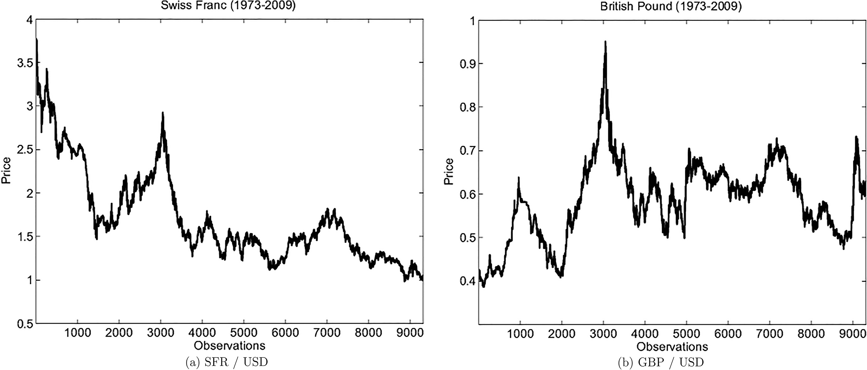
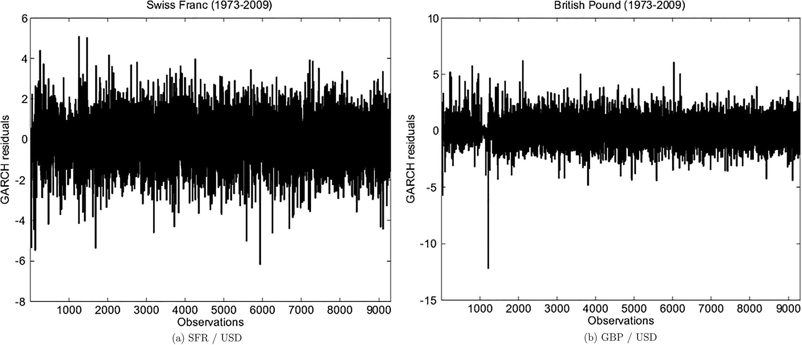
In order to illustrate the benefits of our new construction method, consider two data series from foreign exchange markets (FX-markets) which are available from the PACIFIC Exchange Rate Service (http://pacific.commerce.ubc.ca). In contrast to the volume notation, where values are expressed in units of the target currency per unit of the base currency, the so-called price notation is used within this study which corresponds to the numerical inverse of the volume notation. All values are expressed in units of the base currency per unit of the target currency. For reasons of brevity, we focus on the Swiss Franc/US-Dollar (SFR) and the British Pound/US-Dollar (GBP) henceforth, with daily observations from Feb 2, 1973 to Dec 31, 2009 (see Fig. 1). Instead of using exchange rates itself we consider log-returns (i.e. differences of log-prices), instead which are displayed in Fig. 2.

Figure 2.

Log-returns.

A first insight into the structure of the return series may be gained through Table 3, below. It contains some basic descriptive and inductive statistics of the daily time series: the number of observations ( $N$ ), arithmetic means (Mean), standard deviations (Std), third and fourth standardized moments ( $\mathcal{S},\mathcal{K}$ ). Moreover, tests on normality (i.e. Jarque-Bera test, $\mathcal{JB}$ ) and tests of GARCH effects (i.e. Ljung-Box test for the squared returns $\mathcal{Q}^{2}_{LB}$ with lag $5$ and Engle’s LM test $\mathcal{LM}=N\cdot\mathcal{R}^{2}\lx@stackrel{{\scriptstyle a}}{{\sim}}\chi^{% 2}(k)$ , where $\mathcal{R}^{2}$ is the coefficient of determination of the regression $R_{t}^{2}=\alpha_{0}+\alpha_{1}R_{t-1}^{2}+\ldots+\alpha_{k}R_{t-k}^{2}+% \varepsilon_{t}$ ), complete the summary statistics ( $p$ -values are cited for all statistical tests).

Table 3

Descriptive statistics

	$N$	Mean	Std	$\mathcal{S}$	$\mathcal{K}$	$\mathcal{JB}$	$\mathcal{Q}^{2}_{LB}(5)$	$\mathcal{LM}(5)$
SFR	9307	$-$ 0.014	0.712	$-$ 0.055	6.257	0.000	0.000	0.000
GBP	9307	0.004	0.617	0.144	7.332	0.000	0.000	0.000

Caused by the strong evidence of GARCH effects, we apply a data filter, which means that we fitted GARCH models to the time series in a first and calculate GARCH residuals in a second step.

Figure 3.

GARCH residuals.

Figure 4.

Scatter plot.

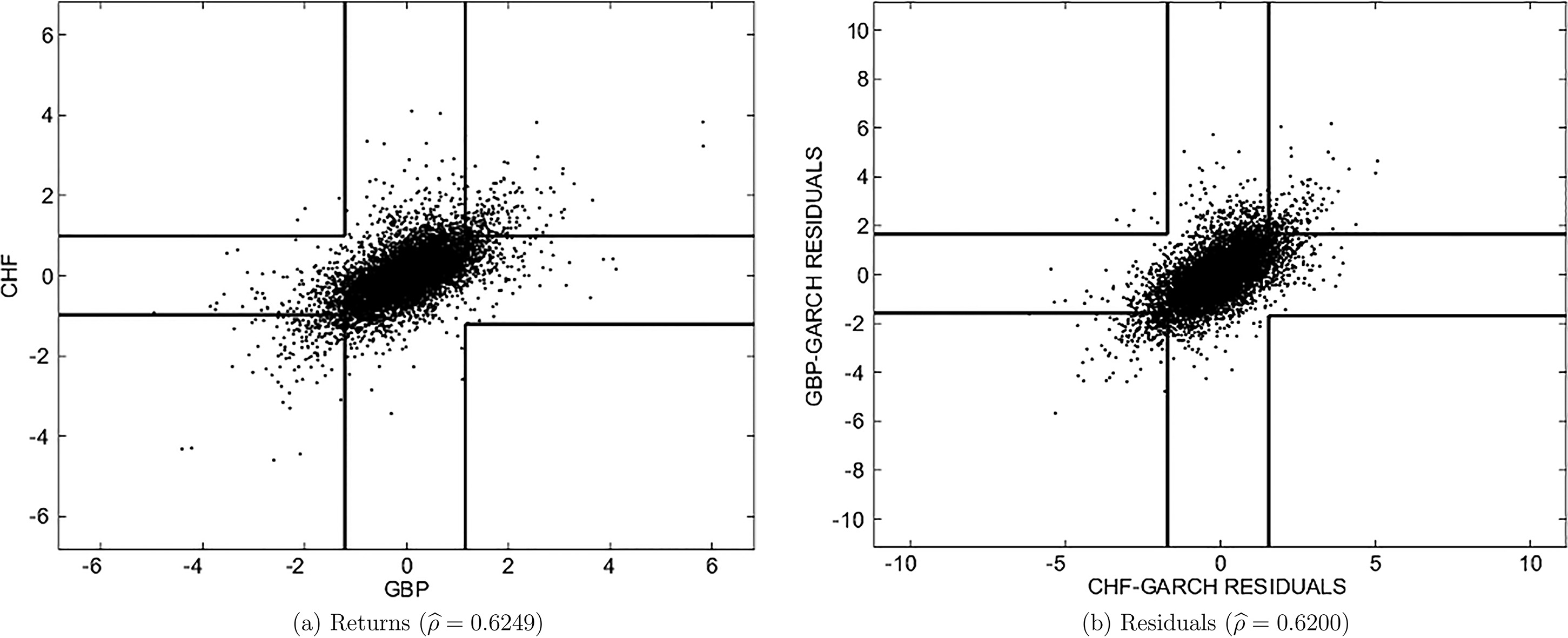
The scatter plot for both returns and GARCH residuals is dedicated to Fig. 4. As to be expected, empirical correlations are essentially equal around $0.62$ in both cases.

9.2 Estimation

Within this work we apply semi-parametric maximum likelihood (SML) estimation which is treated, for example, by Hu (2002) and Genest et al. (1995). Without any parametric assumptions for the margins, the univariate empirical cumulative distribution functions are plugged in the parametric log likelihood function, instead. In other words, after transforming the observed data pairs $(x_{t};y_{t})$ to uniform data pairs $(u_{t};v_{t})$ , the SML estimator of the copula parameter $\theta_{c}$ maximizes the log likelihood function:

$\displaystyle\theta_{c}=\arg\max_{\theta_{c}}\sum_{t=1}^{T}\ln c(u_{t};v_{t};% \theta_{c}).$

9.3 Copulas

The copulas under consideration are chosen on the basis of Theorem 1. Exemplarily, the Clayton copula (denoted by $C_{1}$ ), its rotated counterpart ( $C_{2}$ ) and the Gumbel copula ( $C_{3}$ ) are selected, all of them being exchangeable. For reasons of brevity we introduce some abbreviations, in particular WPM $(C_{1},C_{2};r,\alpha)$ denotes the weighted power mean of the two copulas $C_{1}$ and $C_{2}$ with parameter $r$ and $\alpha$ (see also Table 4, above).

Table 4
Copulas under consideration

Abbr.	Copula	$C(u,v)$	Parameter
C1	Clayton	$(u^{\theta}+v^{\theta}-1)^{1/\theta}$	$\theta>0$
C2	Rotated Clayton	$u+v-1+((1-u)^{\theta}+(1-v)^{\theta}-1)^{1/\theta}$	$\theta>0$
C3	Gumbel	$\exp(-((-\ln(u))^{\theta}+(-\ln(v))^{\theta})^{1/\theta})$	$\theta>1$
C4	WPM(C1,C2; $r,\alpha$ )	see $(1)$	$r>1$
C5	WPM(C1,C3; $r,\alpha$ )	see $(1)$	$r>1$

Finally, Table 5 contains the estimation results from the SML estimation for both original returns and GARCH residuals. In addition to the classical log-likelihood-values ( $\mathcal{LL}$ ) and the parameter estimators we also calculated Akaike’s criterion $AIC=2\cdot LL+\frac{2N(k+1)}{N-k-2}$ which takes the number $k$ of parameter into account. In both cases, the goodness-of-fit can be clearly improve for both WPM copulas under consideration. In addition, parameter estimators for GARCH residuals and return series are very similar. In both cases, WPM outperforms the GAUSS copula and is very close to the Student-t copula with $\nu=3$ degrees of freedom which were added as reference. We chose $\nu=3$ for the Student-t distribution because this is a typical value observed for financial return pairs. Above that, it is guaranteed that at least mean and variance exist. Finally, we observed no significant changes of the log likelihood value if $\nu$ is modified slightly. For data with more skewness one could imagine that C4 and C5 even may outperform the Student-t distribution.

Table 5

Estimation results

Copula	$\mathcal{LL}$	AIC	$\widehat{r}$	$\widehat{\alpha}$	$\widehat{\theta}$
Returns
GAUSS	$2434.0$	$-4824.0$
t( $3$ )	$2752.0$	$-5508.0$
C1	$2122.4$	$-4240.8$	$-$	$-$	$1.1808$
C2	$1896.8$	$-3789.6$	$-$	$-$	$1.1011$
C3	$2422.0$	$-4840.0$	$-$	$-$	$1.7634$
WPM(C1,C2; $r,\alpha$ )	$2642.4$	$-5274.8$	$1.2759$	$0.5484$	$(1.3577,1.8922)$
WPM(C1,C3; $r,\alpha$ )	$2715.9$	$-5421.8$	$5.4267$	$0.4244$	$(0.9502,2.1446)$
GARCH residuals
GAUSS	$2372.0$	$-4747.9$
t( $3$ )	$2630.0$	$-5264.0$
C1	$2061.1$	$-4118.2$	$-$	$-$	$1.1524$
C2	$1816.9$	$-3629.8$	$-$	$-$	$1.0597$
C3	$2319.5$	$-4635.0$	$-$	$-$	$1.7358$
WPM(C1,C2; $r,\alpha$ )	$2556.0$	$-5102.0$	$1.1780$	$0.5665$	$(1.3621,1.8766)$
WPM(C1,C3; $r,\alpha$ )	$2610.5$	$-5211.0$	$3.5132$	$0.4164$	$(1.0628,2.0518)$

10. Conclusion

In general, the weighted power mean of two arbitrary copulas is not necessary a copula again. We establish sufficient conditions which guarantee that this is true and give several examples of new copulas. Moreover, dependence measures for so-called weighted power mean (WPM) copulas are derived and calculated exemplarily for some copulas. Finally, application of WPM copulas to financial return data is given which highlight the flexibility of our new approach.

Footnotes

Acknowledgments

We thank an anonymous reviewer for the thorough review and highly appreciate the comments and suggestions, which significantly contributed to the quality of the publication.

References

Colangelo,

(2006). Some positive dependence orderings involving tail dependence. Working Paper University of Insubria.

Coles,

Heffernan,

, & Tawn,

(1999). Dependence measures for extreme value analyses. Extremes, 2, 339-365.

Durante,

(2009). Construction of non-exchangeable bivariate distribution functions. Statistical Papers, 50, 383-391.

Fischer,

(2010). Dependence modeling: Handbook of vine copulas. Multivariate copulae. Berlin: Springer.

Fischer,

, & Dörflinger,

(2010). A note on a non-parametric tail dependence estimator. Far East J. Theor. Stat., 32, 1-5.

Fischer,

, & Hinzmann,

(2014). A new class of copulas with tail dependence. South African Statist. J., 48, 229-236.

Fischer,

, & Köck,

(2012). Constructing and generalizing given multivariate copulas: A unifying approach. Statistics, 46, 1-12.

Fischer,

Köck,

Schlüther,

, & Weigert,

(2009). An empirical analysis of multivariate copula model. Quantitative Finance, 9, 839-854.

Genest,

Ghoudi,

, & Rivest,

L.-P.

(1995). A semiparametric estimation procedure of dependence parameters in multivariate families of distributions. Biometrika, 82, 543-552.

10.

Heffernan,

(2000). A directory of coefficients of tail dependence. Extremes, 3, 279-290.

11.

Hu,

(2002). Dependence Patterns across Financial Markets: Methods and Evidence. Working Paper, Ohio State University.

12.

Joe,

(1997). Multivariate Models and Dependence Concepts. London: Chapman & Hall.

13.

Ledford,

, & Tawn,

(1996). Statistics for near independence in multivariate extreme values. Biometrika, 83, 169-187.

14.

Lehmann,

(1966). Some concepts of dependence. Ann. Math. Stat., 37, 1137-1153.

15.

Nelsen,

(2006). An Introduction to Copulas. New York: Sprimger.

16.

Nikoloulopoulos,

, & Karlis,

(2010). Modeling multivariate count data using copulas. Commun. Stat. – Simul. Comput., 39, 172-187.

17.

Sklar,

(1959). Fonctions de répartition á n dimensions et leurs marges. Publ. Inst. Statist. University Paris 8, p. 229-231, Paris.

Weighted power mean copulas: theory and application

Abstract

Keywords

1. Introduction

(Counterexamples).

4. Sufficient conditions

.

.

5.1 Extreme-value copulas

.

(WPM-logistic).

5.2 Max-id copulas

.

.

.

.

.

.

.

.

6. Properties of positive dependence and ordering

.

7. Measures of dependence

8. Tail dependence

8.1 Notions of tail dependence

8.2 Strong tail dependence

.

8.3 Weak tail dependence

.

.

.

9.1 Data

9.3 Copulas

Table 4 Copulas under consideration

Footnotes

Acknowledgments

References

Table 4
Copulas under consideration