Empirical comparison of skewed t -copula models for insurance and financial data

Abstract

Skewed $t$ -copulas recently became popular as a modeling tool of non-linear dependence in statistics. In this paper we consider three different versions of skewed $t$ -copulas introduced by Demarta and McNeill; Smith, Gan and Kohn; and Azzalini and Capitanio. Each of these versions represents a generalization of the symmetric $t$ -copula model, allowing for a different treatment of lower and upper tails. Each of them has certain advantages in mathematical construction, inferential tools and interpretability. Our objective is to apply models based on different types of skewed $t$ -copulas to the same financial and insurance applications. We consider comovements of stock index returns and times-to-failure of related vehicle parts under the warranty period. In both cases the treatment of both lower and upper tails of the joint distributions is of a special importance. Skewed $t$ -copula model performance is compared to the benchmark cases of Gaussian and symmetric Student $t$ -copulas. Instruments of comparison include information criteria, goodness-of-fit and tail dependence. A special attention is paid to methods of estimation of copula parameters. Some technical problems with the implementation of maximum likelihood method and the method of moments suggest the use of Bayesian estimation. We discuss the accuracy and computational efficiency of Bayesian estimation versus MLE. Metropolis-Hastings algorithm with block updates was suggested to deal with the problem of intractability of conditionals.

Keywords

Skewed t-copula stock indices time-to-failure tail dependence Bayesian estimation

1. Introduction

1.1 History

Copula models are gaining popularity in modeling non-linear dependence, and especially tail dependence, in multivariate settings. Class of copula model is very rich. The choice of a copula in each particular case is a challenge. Archimedean copulas are very efficient in bivariate case Genest and Rivest (1993), however in transition to higher dimensions, special hierarchical constructions have to be used, such as vines Aas et al. (2008) or nested copulas Hofert and Maechler (2011).

On the other hand, elliptical copulas, such as Gaussian or Student $t$ -copulas, allow for a seamless transition to higher dimensions. The main problem with the Gaussian copula is its inability to model tail dependence. Student $t$ -copula allows for tail dependence, but assumes symmetry of lower and upper tails. This assumption may not be appropriate in cases when lower and upper tails play different roles and have to be analyzed separately. Skewed $t$ -copulas recently became popular as a modeling tool of non-linear dependence, allowing for asymmetric tail dependence. The main issue of dealing with skewed $t$ -copulas is the numerical complexity of estimation and simulation procedures related to them.

1.2 Outline

We consider three different versions of skewed $t$ -copulas introduced by Azzalini et al. (2003), Demarta et al. (2005), and Smith et al. (2012). They represent three different generalizations of the symmetric $t$ -copula model and have their own advantages and disadvantages. All three have been used in a variety of settings. We will make an effort to compare the performance of these three models for specific applications, similar to how it was done in Yoshiba (2018). The main objective of the paper is to use common model selection tools to determine, which of the skewed $t$ -copulas prove to be more appropriate for practical use and whether they provide an advantage when compared to the symmetric Student $t$ and Gaussian copulas. In our empirical study, we do not provide model validation, nor we address a separate issue of possible copula model mis-specification due to the choice of the marginals, see Fantazzini (2009). We also do not provide analysis of model identifiability for skewed $t$ -copulas which would be better addressed by a simulation study. For the sake of technical simplicity and easy interpretation, we we will use bivariate examples, for which symmetric $t$ -copulas are known to outperform Archimedean models, see Shemyakin and Kniazev (2017). All the suggested methods of model selection can be used in multivariate cases of dimension higher than 2.

One of the applications is quite traditional for copula studies. It deals with the joint distribution of international stock indices. Daily percentage returns on indices are filtered using standard ARIMA/GARCH methodology and copulas are used to model the dependence structure of their residuals (normalized innovations). Asymmetric tail behavior of financial variables is known since Longin and Solnik (2001), and the use of Student $t$ -copulas was suggested in Mashal and Zeevi (2002). We select two indices to illustrate the performance of skewed $t$ -copulas as compared to Gaussian and symmetric Student $t$ -copula.

We will also consider a case study of related failures of vehicle components under the warranty period. Study in Baik and Mhitarian (2006) analyzed failures in such Hyundai Accent engine components as spark plug assembly and ignition coil assembly. The data were collected during the 5-year warranty period. Lower and upper tails correspond to related failures happening in the beginning and the end of the warranty period, and have very distinct roles in risk and performance analyses Shemyakin and Kniazev (2017).

For these two empirical studies, three skewed $t$ -copulas are compared to Gaussian and symmetric Student $t$ -copulas. Instruments of model comparison include information criteria, goodness-of-fit, and tail dependence. In order for this comparison to become possible, we need to estimate copula parameters for each of the models. If we use the method of maximum likelihood or the method of moments, we face multiple technical problems as demonstrated by Yoshiba (2018). Therefore we choose a different route, using Bayesian estimation, as also suggested in Smith et al. (2012). It promises certain degree of computational efficiency, but there still exist some non-trivial problems on this route, including the choice of priors and computer implementation of MCMC procedures.

The main focus of the paper is an effort to combine the advantages of Bayesian approach to estimation with the flexibility of copula modeling. Sergey Artemievich Aivazian was one of the pioneers of both in Russian statistical and econometric literature. In Aivazian and Mhitarian (1998) and Aivazian and Mhitarian (2015), Aivazian and his collaborators introduced analysis of dependence including copulas in econometric studies. In Aivazian (2008) he attracted attention of econometricians to the intricacies of Bayesian approach. One of the co-authors of the present paper had many insightful discussions with Aivazian regarding these two areas of modern statistics.

1.3 Paper structure

Section 2 contains basic description of the considered copula classes. Section 3 discusses specifics of model comparison criteria and covers estimation methodology including elicitation of priors and the choice of MCMC procedures. Sections 4 and 5 are dedicated to empirical studies and the results obtained for two applications.

2. Elliptical copulas

The elliptical distribution $Q_{d,R}$ of a random vector $\bm{t}=(t_{1},\ldots,t_{d})$ can be defined by its joint density function

$\displaystyle|\Sigma|^{-1/2}k((t-\mu)^{\rm T}\Sigma^{-1}(t-\mu)),$

where $\mu$ is a $d\times 1$ vector of means, $\Sigma$ is a positively defined $d\times d$ covariance matrix, and $k(x)$ is some non-negative function of one variable integrable over the entire real line. Matrix $\Omega$ with elements $\Omega_{ij}={\Sigma_{ij}}/{\sqrt{\Sigma_{ii}\times\Sigma_{jj}}}$ is the correlation matrix determining all pairwise associations between the components of the random vector $\bm{t}$ . Define also by $Q_{i}(t_{i})$ the marginal distribution of $t_{i}$ . Then we can define an elliptical copula as

$\displaystyle C(t_{1},\ldots,t_{d};\Omega)=Q_{d,\Omega}(Q^{-1}_{1}(t_{1}),% \ldots,Q^{-1}_{d}(t_{d})).$ (1)

The most popular elliptical copula is the Gaussian copula, which, combined with marginal distributions $t_{i}=F_{i}(u_{i})$ of the data vector $U=(U_{1},\ldots,U_{d})$ , defines the joint distribution $H(u)$ of vector $U$ as

$\displaystyle H(u)=C_{G}(t_{1},\ldots,t_{d};\Omega)=\Phi_{d,\Omega}(\Phi^{-1}(% F_{1}(u_{1})),\ldots,\Phi^{-1}(F_{d}(u_{d}))),$ (2)

where $\Phi(u)$ is the standard normal distribution and $\Phi_{d,R}$ is $d$ -variate normal with zero mean, unit variances and correlation matrix $R$ . Off-diagonal elements of matrix $\Omega$ describe pairwise associations, so the strength of the association may differ for different pairs of components of vector $\bm{U}$ .

Another popular choice of an elliptical copula is Student’s $t$ -copula Demarta and Mc Neil (2005),

$\displaystyle H(u)=C_{t}(t_{1},\ldots,t_{d};\Omega,\nu)=T_{d,\Omega,\nu}(T_{% \nu}^{-1}(F_{1}(u_{1})),\ldots,T_{\nu}^{-1}(F_{d}(u_{d}))),$ (3)

where $T_{\nu}(x)$ is a $t$ -distribution with $\nu$ degrees of freedom, and $T_{d,\nu,R}$ is $d$ -variate $t$ -distribution with $\nu$ degrees of freedom and correlation matrix $\Omega$ .

The Azzalini-Capitanio skewed $t$ -copula defined in Azzalini and Mhitarian (2003) (further: AC) can be represented as

$\displaystyle H(u)=C_{\rm AC}(t_{1},\ldots,t_{d};\Omega,\delta,\nu)$ (4) $\displaystyle=AC_{d,\Omega,\alpha,\nu,R}(AC_{\gamma_{1},\nu}^{-1}(F_{1}(u_{1})% ),\ldots,AC_{\gamma_{d},\nu}^{-1}(F_{d}(u_{d}))),$ (5)

where $AC_{\gamma,\nu}(x)$ is a skewed $t$ -distribution with skewness $\gamma$ and $\nu$ degrees of freedom, and $AC_{d,\Omega,\alpha,\nu}$ is $d$ -variate skewed $t$ -distribution with $\nu$ degrees of freedom, skewness vector $\alpha$ and correlation matrix $\Omega$ .

Joint density for d-variate skewed $t$ -distribution $AC_{d,\Omega,\alpha,\nu}$ can be defined as

$\displaystyle g(x,\Omega,\alpha,\nu)=2t_{d,\nu}(x;\Omega)T_{1,\nu+d}\left(% \alpha^{\rm T}x\sqrt{\frac{\nu+d}{x^{\rm T}\Omega^{-1}x+\nu}}\right),$ (6)

where $t_{d,\nu}(x;\Omega)$ is the $d$ -variate $t$ -density with the correlation matrix $\Omega$ and degrees of freedom $\nu$ :

$\displaystyle t_{d,\nu}(x;\Omega)=\frac{\Gamma((\nu+d)/2)}{(\pi\nu)^{d/2}% \Gamma(\nu/2){|\Omega|}^{1/2}}\left(1+\frac{x^{\rm T}\Omega^{-1}x}{\nu}\right)% ^{-(\nu+d)/2},$

and $T_{1,\nu}(x)$ is the univariate symmetric cumulative $t$ -distribution function with $\nu$ degrees of freedom.

As demonstrated in Yoshiba (2018), there is a simple relationship between skewness vector $\delta$ of the copula and the skewness parameters $\alpha$ and $\gamma_{i}$ used in definition Eq. (4):

$\displaystyle\alpha=\frac{\Omega^{-1}\delta}{\sqrt{1-\delta^{\rm T}\Omega^{-1}% \delta}},\gamma_{i}=\frac{\delta_{i}}{\sqrt{1-\delta_{j}^{2}}}.$ (7)

Another way to define a skewed $t$ -copula is based on characterization of a $d$ -dimensional skewed- $t$ by a function of random variables with simpler distributions. One such characterization was suggested in Demarta and Mc Neil (2005), where skewed $t$ -distribution is defined by r.v.

$\displaystyle X=\gamma V^{-1}+ZV^{-1/2},$ (8)

where $Z\sim N_{d}(0,\Sigma)$ , $V\sim\Gamma(\nu/2,\nu/2)$ , and $\gamma$ is the skewness vector. An advantage of this approach is representation of all the marginals of $X$ as univariate skewed- $t$ with skewness parameters $\gamma_{i}$ . We will call it Demarta-McNeill copula (further: DM).

The third option suggested in Smith et al. (2012) (further: Smith-Gan-Kohn or SGK copula) characterizes skewed $t$ -distribution by r.v.

$\displaystyle X=\frac{\Gamma|W|+Z}{V^{1/2}},$ (9)

where $Z\sim N_{d}(0,\Sigma)$ , $W\sim N_{d}(0,I)$ , $V\sim\Gamma(\nu/2,\nu/2)$ , and $\Gamma$ is a diagonal matrix $\Gamma=diag(\gamma_{1},\ldots\gamma_{d})$ . It shares with DM copula the property of marginal pd.f. being univariate skewed- $t$ with skewness defined by $\gamma_{i}$ .

In the following section we will describe the criteria we will use for model selection between these three classes of copulas: AC, DM, and SGK, using symmetric Gaussian copula and $t$ -copula as benchmarks. Then we will characterize the methods of parametric estimation.

3. Criteria of model selection and methods of estimation

Non-nested models obtained for different definitions of skewed $t$ -copulas are compared via

•
Likelihood-based information criteria (AIC and BIC).
•
MCMC-based information criterion (DIC).
•
Goodness-of-fit (Kolmogorov-Smirnov distance).
•
Tail dependence.

Standard definitions of information criteria in terms of likelihood function of the data $x$ and parameter $\theta$ with likelihood $L(x;\theta)$ are: deviance $D(\theta)=-2\ln L(x;\theta)$ , Akaike information criterion $\textit{AIC}=D(\hat{\theta})+2k$ ; Bayesian (Schwarz) information criterion $\textit{BIC}=D(\hat{\theta})+k\log n$ , where $\hat{\theta}$ is the value of MLE, $k$ is the number of parameters and $n$ is the sample size. We will follow the suggestion of Burnham and Anderson (2002) also supported by a recent survey study Portet (2020) that information criteria AIC and BIC can be used for non-nested models, which makes them a convenient model selection tool.

Another information criterion conveniently used in Bayesian framework is DIC (deviance information criterion) defined in Spiegelhalter et al. (2002) for Markov chain Monte Carlo procedures as

$\displaystyle\textit{DIC}=2\bar{D}-D(\bar{\theta}),$ (10)

where $\bar{\theta}$ is the deviance of the sample posterior mean and $\bar{D}$ is the sample posterior mean of the deviance.

Kolmogorov-Smirnov distance between the empirical c.d.f. $F_{n}^{}(x)$ and the model c.d.f. $F_{0}(x)$ is defined as

$\displaystyle d_{KS}(F_{n}^{}(x),F_{0}(x))=\sup|F_{n}^{}(x)-F_{0}(x)|$ (11)

and can be used for goodness-of-fit testing in one-dimensional case. In multidimensional situations such use is not transparent since the test statistic cannot be determined in closed form and some kind of Monte Carlo simulation has to be applied. However, the values of $d_{KS}$ can be compared for different models and different estimation methods, and this relative analysis can provide a tool of model selection Shemyakin and Kniazev (2017).

Lower tail dependence $\lambda_{L}$ and upper tail dependence $\lambda_{U}$ for a two-dimensional copula $C(u,v)$ may be defined as

$\displaystyle\lambda_{L}=\lim_{u\downarrow 0}\frac{C(u,u)}{u},\lambda_{U}=\lim% _{u\uparrow 1}\frac{2u-1-C(1-u,1-u)}{1-u}.$ (12)

For Gaussian copula $\lambda_{L}=\lambda_{U}=0$ and for Student $t$ -copula with degrees of freedom $\nu$ and correlation $\rho$

$\displaystyle\lambda_{L}=\lambda_{U}=T_{\nu+1}\Bigg{(}-\sqrt{\nu+1}\sqrt{\frac% {1-\rho}{1+\rho}}\Bigg{)}.$

Similar formulas can be obtained for skewed $t$ -copulas interms of their parameters. If there is a good way to estimate tail dependence empirically, we can comapre these values with model values and use it as another tool of model selection. If we follow Bernard et al. (2013), we can define for $q$ -quantile and copula $C(u,v)$ the model-induced lower tail exceedance* in terms of Kendall’s $\tau$ :

$\displaystyle\tau_{L}(q)=\frac{4\int_{0}^{q}\int_{0}^{q}C(u,v){\rm d}C(u,v)}{C% ^{2}(q,q)},$ (13)

which then can be compared with the empirical conditional concordance $\tau(U,V|U\leqslant q,V\leqslant q)$ .

Brechmann in Brechmann (2010) suggested a handy graphical measure of tail dependence called tail cumulation, defined for quantile $q$ and bivariate sample $(u_{i},v_{i})\in[0,1]^{2},i=1,\ldots,n$ :

$\displaystyle\gamma_{L}(q)=\frac{1}{n}\sum_{i=1}^{n}I_{u_{i}\leqslant\sqrt{q},% v_{i}\leqslant\sqrt{q}}-q,$ (14)

which also makes it possible to match copula models with empirical pseudo-observations $(u,v)$ . Unfortunately this approach is not able to clearly distinguish different tail dependence patterns, so it has to be used cautiously. Upper tail exceedance and tail cumulation can be defined similarly.

Maximum likelihood estimation for skewed $t$ -copula models faces some serious technical issues (see Yoshiba (2018)). Therefore we make an effort to resolve some of these problems using a Bayesian approach. We implement Bayes estimation numerically, using independent priors for parameters: Wishart prior for the correlation matrix, exponential prior and Poisson prior for the number of degrees of freedom, and multivariate Laplace prior for the skewness parameters as well as non-informative uniform priors. Due to intractability of the conditionals, which is characteristic for copula models, we choose a modification of Markov chain Monte Carlo methods: block-wise random walk Metropolis-Hastings algorithm. The accept/reject step of the algorithm also assumes checking additional conditions required for correct definition of skewed $t$ -copulas, such as existence of skewness parameters in Eq. (6). Approximate Bayesian computing (ABC) is also to be considered in future. We compare the Bayesian results with the results of maximum likelihood estimation.

There are some technical problems with the evaluation of the likelihood function. In most cases, we cannot find the analytical form of the cumulative distribution function of skewed $t$ -copulas, therefore we have to implement numerical integration. An efficient way to reduce the computation time while maintaining high degree of accuracy is to use a monotone interpolator Joe (2014). We apply piecewise cubic Hermitian interpolating polynomial with 250 interpolation points following Yoshiba (2018).
4. Stock index returns

We consider daily logarithmic returns of nine different stock indices and their combinations for the period of 5 years (January 2011 to December 2015). The chosen example includes HSI (Hang Seng) and S&P500 (Standard and Poor’s 500). After basic filtration using ARIMA/GARCH methodology, we model copula association of the residuals (normalized innovations) of these two time series, assuming skewed $t$ -distribution for the marginals.

Let us consider times $t=1,2,\ldots,T$ , where the time increment will correspond to 1 day and define daily log-returns for indices $j=1,2$ as $S_{j}^{(t)}$ . We will estimate parameters in ARIMA $(p,d,q)$ model as $\phi_{ji},\theta_{ji}$ , where

•
$D_{j}^{(t)}=\Delta^{\rm d}(S_{j}^{(t)})$ , where $\Delta$ is the difference operator, $\Delta f^{(t)}=f^{(t)}-f^{(t-1)}$ , $\Delta^{\rm d}f^{(t)}=\Delta^{d-1}f^{(t)}-\Delta^{d-1}f^{(t-1)}$ reflecting possible non-stationarity;
•
$D_{j}^{(t)}=\phi_{j0}+\sum_{i=1}^{\rm p}\phi_{ji}D_{j}^{(t-i)}+\sum_{i=1}^{\rm q% }\theta_{ji}\varepsilon_{j}^{(t-i)}+\varepsilon_{j}^{(t)}$ , as in ARIMA $(p,d,q)$ .
•
$u_{j}^{(t)}=\frac{\varepsilon_{j}^{(t)}}{\sigma_{j}^{(t)}}$ , where $\sigma_{\rm t}^{2}=\omega+\alpha_{1}\varepsilon_{t-j}^{2}+\beta_{1}\sigma_{t-j% }^{2}$ is the variable volatility estimated by GARCH(1,1),
•
Innovations in GARCH model $u_{j}^{(t)}$ are assumed to be independent and obtain skewed $t$ -distribution with skewness parameter $\gamma$ and degrees of freedom $\nu$ as defined in Fernandez and Steel (1998).

We also considered higher orders of GARCH, which could provide a good fit for data, but they also bring about over-parameterization. In order to provide model diagnostics, we used sign bias test, Nyblom stability test, weighted ARCH LM test, and weighted Ljung-Box test. Based on this study, we suggest the following models: for S&P500 ARIMA (3,0,0)/GARCH(1,1), $p=3,d=0,q=0$ and for HSI ARIMA(0,0,0)/GARCH(1,1) $p=0,d=0,q=0$ with the parameter values summarized in Tables 1 and 2. For our study it was important to use the same marginal models for all copulas under consideration.

Table 1
Estimates of ARIMA/GARCH parameters for HSI

Parameter Estimate St.error $t$ -value $p$ -value

$\phi_{0}$ 0.0001 0.0003 0.5176 0.6047

$\omega$ 0.0000 0.0000 0.8943 0.3711

$\alpha_{1}$ 0.0537 0.0196 2.74 0.0061

$\beta_{1}$ 0.9319 0.0237 39.26 0.0000

$\gamma$ 0.9607 0.0370 25.96 0.0000

$\nu$ 6.10 0.99 6.19 0.0000

Table 2
Estimates of ARIMA/GARCH parameters for S&P500

Parameter Estimate St.error $t$ -value $p$ -value

$\phi_{0}$ 0.0006 0.0002 3.203 0.0013

$\phi_{1}$ $-$ 0.0612 0.03381 $-$ 1.973 0.0481

$\phi_{2}$ $-$ 0.0516 0.0304 $-$ 1.697 0.0896

$\phi_{3}$ $-$ 0.0594 0.0296 $-$ 2.008 0.0447

$\omega$ 0.0000 0.0000 1.028 0.3040

$\alpha_{1}$ 0.1691 0.0314 5.391 0.0000

$\beta_{1}$ 0.7877 0.050 15.75 0.0000

$\gamma$ 0.8338 0.0365 22.87 0.0000

$\nu$ 6.61 1.74 3.792 0.0001

Estimates of copula parameters for the residuals of daily index log-returns are summarized in Table 3, where both MLE and Bayesian methods are used for each of the models. Parameters estimated include correlation $\rho$ , degrees of freedom $\nu$ , and two components of the skewness vector: $\gamma=(\gamma_{1},\gamma_{2})$ . Estimation was performed in R using specialized packages Kojadinovic and Yan (2010).

Table 3
Estimates of copula parameters for residuals of HSI and S&P500

Model/method MLE Bayes

$\rho$ $\nu$ $\gamma_{1}$ $\gamma_{2}$ $\rho$ $\nu$ $\gamma_{1}$ $\gamma_{2}$

Gaussian 0.258 0.260

Student $t$ 0.257 45.9 0.246 8.9

AC 0.353 29.4 $-$ 0.324 $-$ 0.979 0.247 5.7 0.013 0.030

DM 0.225 31.2 $-$ 0.641 $-$ 0.812 0.252 10.5 0.004 $-$ 0.026

SGK 0.250 12.0 0.045 $-$ 0.011 0.289 11.9 0.036 0.068

Results in Table 3 for various models are consistent other than MLE for AC copula, which seems to substantially overestimate the correlation. Number of degrees of freedom is smaller for Bayes estimates, which reflects the intent of being conservative and penalizing high values of degrees of freedom in the prior. Difference in the estimates of skewness parameters is explained by different definitions of skewness in three models considered.

Table 4
Information criteria for models of index returns

Model/method MLE Bayes

-AIC -BIC -AIC -BIC -DIC

Gaussian 80 74 80 74 78

Student $t$ 78 68 71 61 60

AC 77 57 54 34 50

DM 76 56 70 50 68

SGK 73 53 66 46 49

Table 4 contains negative values for AIC and BIC rounded to nearest integers, therefore the higher values correspond to better models. For Bayes estimates, we also provide DIC values. The highest value in each column corresponding to the best model is boldfaced. It is clear that the most parsimonious Gaussian model works better in all cases, therefore the information criteria approach does not support the use of skewed models. One should notice that the values in Table 4 are expected to be higher for MLE than for Bayes, since both AIC and BIC are explicitly constructed based on the likelihood function.

Table 5
Kolmogorov-Smirnov distance for models of index returns

Model/method MLE Bayes

Gaussian 0.0346 0.0342

Student $t$ 0.0347 0.0365

AC 0.0358 0.0364

DM 0.0378 0.0340

SGK 0.0329 0.0176

As we see from Table 5, for skewed $t$ -copulas MLE and Bayesian estimation provides close values of Kolmogorov-Smirnov statistic between the model and empirical c.d.f-s, defined in Eq. (10). Comparing AC, DM, and SGK, we can give slight edge to the performance of SGK copula. However, overall goodness-of-fit does not sufficiently discriminate against Gaussian and symmetric $t$ -copula, so this criterion, characterizing overall goodness-of-fit, may be not as important as the tail behavior.

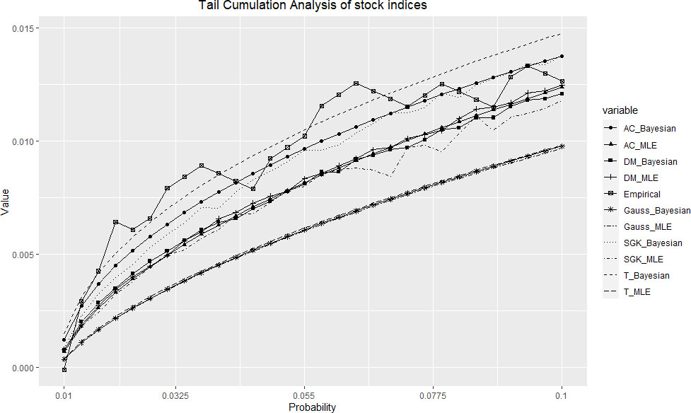
We will illustrate the tail fit graphically with the lower tail cumulation Eq. (13) in Fig. 1. Lower tails for index returns are certainly more important from a risk management point of view than the upper tails. What one could easily foresee, is a relatively poor fit of Gaussian model for all quantile values included in the graph ( $q=0.01$ to $q=0.1$ ). The upper line on the chart representing empirical values, substantially exceeds most model values, though both AC and SGK skewed models along with symmetric Student $t$ -copula suggest a satisfactory fit for Bayes estimates. Lower number of degrees of freedom characterizing Bayes estimates in Table 3 may explain the fact that Bayes estimates provide more realistic models of the tail behavior than MLE.

Figure 1.
Lower tail cumulation for index returns.

5. Related failures of vehicle components

Parameter	Estimate	St.error	$t$ -value	$p$ -value
$\phi_{0}$	0.0001	0.0003	0.5176	0.6047
$\omega$	0.0000	0.0000	0.8943	0.3711
$\alpha_{1}$	0.0537	0.0196	2.74	0.0061
$\beta_{1}$	0.9319	0.0237	39.26	0.0000
$\gamma$	0.9607	0.0370	25.96	0.0000
$\nu$	6.10	0.99	6.19	0.0000

Parameter	Estimate	St.error	$t$ -value	$p$ -value
$\phi_{0}$	0.0006	0.0002	3.203	0.0013
$\phi_{1}$	$-$ 0.0612	0.03381	$-$ 1.973	0.0481
$\phi_{2}$	$-$ 0.0516	0.0304	$-$ 1.697	0.0896
$\phi_{3}$	$-$ 0.0594	0.0296	$-$ 2.008	0.0447
$\omega$	0.0000	0.0000	1.028	0.3040
$\alpha_{1}$	0.1691	0.0314	5.391	0.0000
$\beta_{1}$	0.7877	0.050	15.75	0.0000
$\gamma$	0.8338	0.0365	22.87	0.0000
$\nu$	6.61	1.74	3.792	0.0001

Model/method	MLE	Bayes
Gaussian	0.258				0.260
Student $t$	0.257	45.9			0.246	8.9
AC	0.353	29.4	$-$ 0.324	$-$ 0.979	0.247	5.7	0.013	0.030
DM	0.225	31.2	$-$ 0.641	$-$ 0.812	0.252	10.5	0.004	$-$ 0.026
SGK	0.250	12.0	0.045	$-$ 0.011	0.289	11.9	0.036	0.068

Model/method	MLE	Bayes
Gaussian	80	74	80	74	78
Student $t$	78	68	71	61	60
AC	77	57	54	34	50
DM	76	56	70	50	68
SGK	73	53	66	46	49

Model/method	MLE	Bayes
Gaussian	0.0346	0.0342
Student $t$	0.0347	0.0365
AC	0.0358	0.0364
DM	0.0378	0.0340
SGK	0.0329	0.0176

We consider open source data presented in a case study Baik and Mhitarian (2006) including a dataset of manufacturer warranty claims on Hyundai Accent from 1996 to 2000. The critical components chosen to illustrate related failures are engine components: spark plug embassy and ignition coil assembly. The total of 467 failures were recorded during the warranty period. The time in days until failure (first repair or replacement) is recorded for each of two components. Copulas are used to model the association between the time-to-failure variables measured in days with Weibull distribution model assumed for the marginals.

Notice that the use of Archimedean copulas including Clayton’s and Gumbel-Hougaard copulas can be suggested for bivariate data with strong tail dependence, and an empirical study of Archimedean copulas for vehicle failures can be found in Wifvat et al. (2020). However, as Shemyakin and Kniazev (2017) suggests, even symmetric $t$ -copulas outperform one-tailed Archimedean copulas for vehicle component data, therefore elliptical copulas may provde for a better model.

Estimates of copula parameters for time-to-failure of two chosen vehicle components are summarized in Table 6, where both MLE and Bayesian methods are used for each of the models. Parameters estimated include correlation $\rho$ , degrees of freedom $\nu$ , and the skewness vector $\gamma=(\gamma_{1},\gamma_{2})$ .

Table 6
Estimates of copula parameters for time-to-failure of engine components

Model/method	MLE				Bayes
	$\rho$	$\nu$	$\gamma_{1}$	$\gamma_{2}$	$\rho$	$\nu$	$\gamma_{1}$	$\gamma_{2}$
Gaussian	0.787				0.783
Student $t$	0.902	1.43			0.893	1.37
AC	0.909	2.01	$-$ 0.058	0.298	0.925	2.01	$-$ 0.021	0.145
DM	0.929	4.00	0.072	0.186	0.931	4.05	0.058	0.166
SGK	0.909	8.00	0.012	0.087	0.876	11.00	0.066	0.121

Table 7

Information criteria for models of engine component failure

Model/method	MLE		Bayes
	-AIC	-BIC	-AIC	-BIC	-DIC
Gaussian	492	488	492	488	492
Student $t$	834	826	833	825	829
AC	963	946	961	945	951
DM	818	801	816	799	783
SGK	698	682	654	638	612

Figure 2.

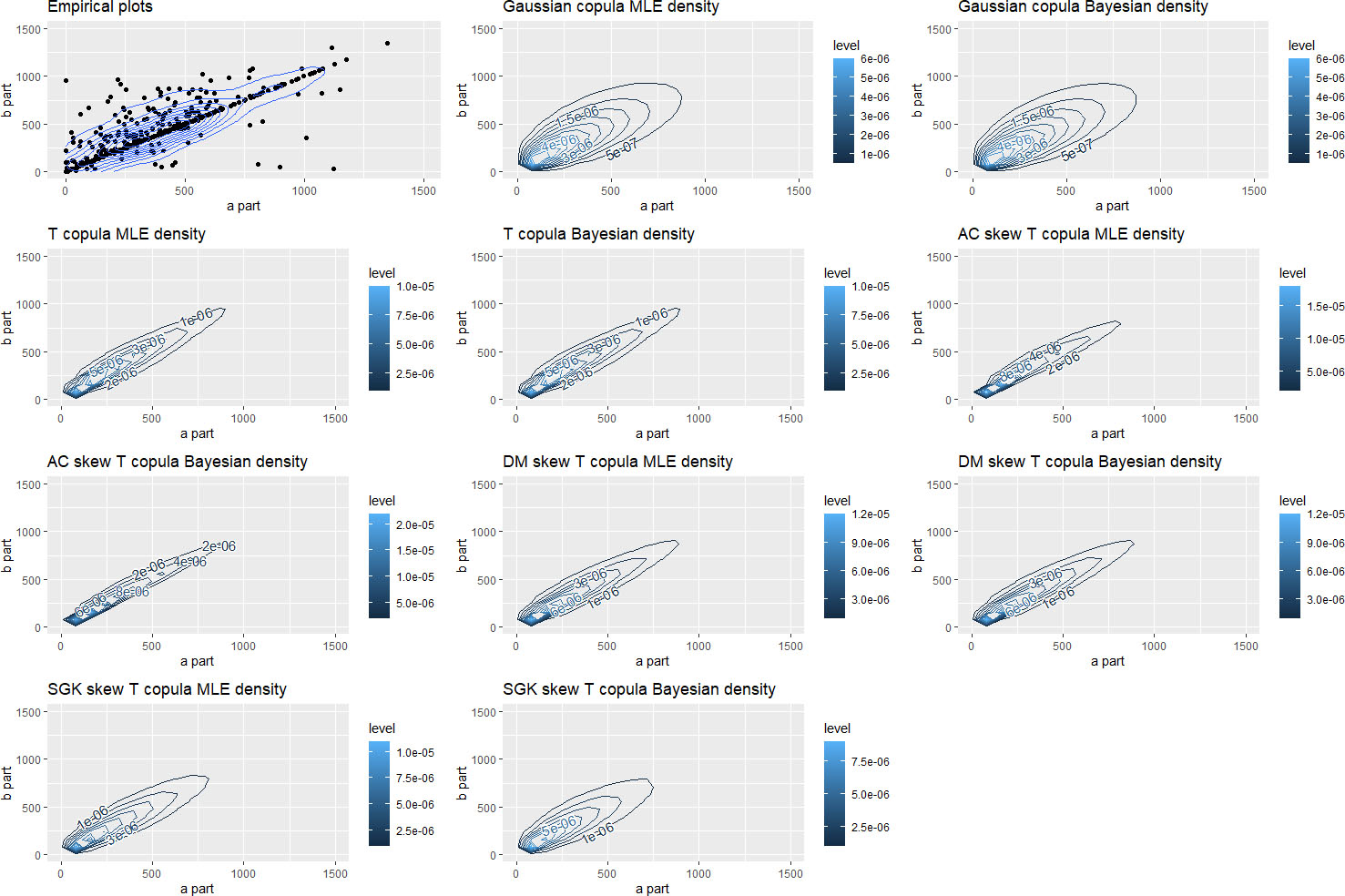
Scatterplot and model contour plots for joint distribution of times-to-failure of engine components.

The vehicle component failure data are very different from the index return example since they clearly exhibit both lower and upper tails, which have very distinct roles of representing related failures early (low tail) or late (upper tail) in the warranty period. Therefore it is expected that skewed $t$ -copulas might substantially outperform both Gaussian and Student $t$ -copula benchmark models. The role of two tails is expressed in the low number of degrees of freedom (for both Bayes estimation and MLE). The asymmetry of these two tails can be observed in Fig. 2, where the upper left panel corresponds to the empirical joint distribution of the lifetimes of spark plug embassy and ignition coil assembly.

Table 7 contains negative AIC and BIC values, and also DIC for Bayes estimates (the higher number the better), which clearly indicate the preference given to AC copula model (the highest values in each column are boldfaced). Gaussian model is definitely outperformed, since joint tails in this dataset are well established (see also Fig. 2).

Comparison of Kolmogorov-Smirnov distances in Table 8 does not suggest any advantage of skewed models since Gaussian copula provides for the best overall fit. This is another example of low sensitivity of KS statistic to the joint distribution tails.

Table 8

Kolmogorov-Smirnov distances for models of engine component faliures

Model/method	MLE	Bayes
Gaussian	0.1005	0.1001
Student $t$	0.1006	0.1002
AC	0.1007	0.1049
DM	0.1032	0.1030
SGK	0.1045	0.1075

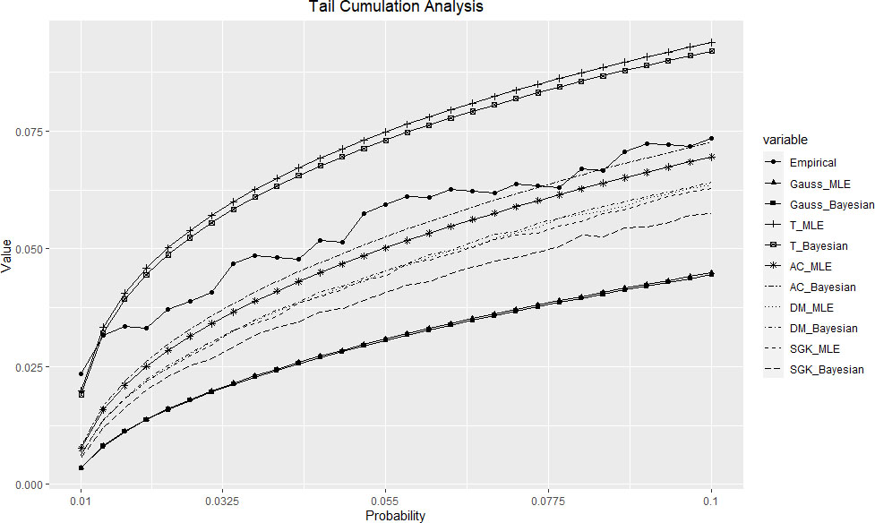
Graphical comparison of lower tail cumulation in Fig. 3 reveals some interesting patterns. It looks like AC copula provides a better model for empirical lower tail than any other model. However, symmetric Student $t$ -copula is probably the second best, and it even overestimates the empirical tail. It can be explained by the fact that Student $t$ -copula assumes symmetry of the tails, and thus the association detected in the upper tail also affects the estimates for the lower tail in the upward direction.

Figure 3.

Lower tail cumulation for vehicle components.

6. Conclusions

Two examples we considered may illustrate the problems of applying skewed $t$ -copula models to financial and insurance data. In both cases introduction of skewness to copula models creates both conceptual and technical issues. One of the conceptual issues is a proper choice of skewness structure, and it is a difficult choice. We considered three different constructions, and each of them has their own advantages. A technical issue is computational difficulty of estimation in skewed $t$ -copula models. One of possible avenues is the use of Bayesian methods, which may help to overcome some of the technical problems. It looks like the main benefit of using skewed $t$ -copulas is a better fit of distribution tails.

The example of index returns demonstrates that the advantage of using skewed $t$ -copulas may be questionable, not improving the fit of benchmark Gaussian and symmetric Student $t$ -copula models to the desired extent. Information criteria are lukewarm to skewed $t$ -constructions, while both KS goodness-of-fit and tail cumulation analysis suggest a slight advantage of Azzalini-Capitanio AC and Smith-Gahn-Kohn copulas.

On the contrary, vehicle component analysis demonstrates that in the presence of strong tail dependence there is a clear benefit of using skewed $t$ -models, which is indicated by information criteria, though it is not registered when comparing Kolmogorov-Smirnov distances. Out of three suggested versions, AC copula seems to also provide the best tail fit.

In future, it would be interesting to extend the scope of this empirical study to dimensions higher than 2. Also, more comprehensive analysis of both upper and lower tails may demonstrate efficiency and practicality of skewed $t$ -copula models when applied to particular data structure. Index returns and joint times-to-failure of engine components are just two of many possible settings, which may require individual approach to model selection.

The authors would like to acknowledge the help of colleagues Yankai Gao, Xiaowen He and Chengjiang Ren with computer implementation of the estimation procedures.

References

Aas

Czado

Frigessi

& Bakken

(2008). Pair-copula constructions of multiple dependence. Insurance: Mathematics and Economics, 44, 182-198.

Aivazian

, & Mhitarian

(1998). Applied statistics and foundations of econometrics Moscow, Unity, In Russian.

Aivazian

(2008). Bayesian approach to econometric analysis. Applied Econometrics, 1(9), 93-130. In Russian.

Aivazian

& Fantazzini

(2015). Modeling joint distributions via copula functions. In: Econometrics-2. Advanced Course with Applications to Finance Moscow, HSE, In Russian.

Azzalini

& Capitanio

(2003). Distributions generated by perturbation of symmetry with emphasis on a multivariate skew t-distribution. Jourmal of the Royal Statistical Society. Series B, 65(2), 367-389.

Baik

, & Jo

(2006). Non-parametric analysis of wrranty data on engines: Case study. J of the Korean Society for Qualty Management, Seoul, 34(1), 40-47.

Bernard

Brechmann

E. C.

, & Czado

(2013). Statistical assessment of systemic risk measures. In: Handbook of Systemic Risk, Eds: Fouque

J. P.

& Langsam

J. A.

, Cambridge University Press, Business and Economics, 165-179.

Brechmann

E. C.

(2010). Truncated and simplified regular vines and their applications. Technisches UniversitÃ¤t MÃ¼nchen, Zentrum Mathematik, 1-207.

Burnham

K. P.

, & Anderson

D. R.

(2002). Model Selection and Multimodel Inference: A Practical Information-Theoretic Approach (2nd ed.), Springer-Verlag, ISBN 0-387-95364-7.

10.

Demarta

& Mc Neil

(2005). The t-copulas and related copulas. International Statist. Review, 73, 111-129.

11.

Fantazzini

(2009). The effects of misspecified marginals and copulas on computing the value at risk: A Monte Carlo study. Computational Statistics and Data Analysis, 53(6), 2168-2188.

12.

Fernandez

, & Steel

M. F. J.

(1998). On Bayesian modeling of fat tails and skewness. J. Amer. Statist. Assoc., 93(441), 359-371.

13.

Genest

, & Rivest

L. P.

(1993). Statistical inference procedures for bivariate Archimedean copulas. J Amer Statist Assoc, 88, 1034-1043.

14.

Hofert

& Maechler

(2011). Nested Archimedean copulas meet R. Journal of Staistical Software, 39(9), 1-20.

15.

Joe

(1997). Multivariate models and dependence concepts, Chapman & Hall, London.

16.

Joe

(2014). Dependence Modeling with Copulas, Chapman & Hall/CRC, London.

17.

Justel

Pena

, & Zamar

(1997). A multivariate Kolmogorov-Smirnov test of goodness of fit. Statistics & Probability Letters, 35(3), 251-259.

18.

Kojadinovic

, & Yan

(2010). Modeling multivariate distributions with continuous margins using the copula R package. Journal of Statistical Software, 34(9), 1-20.

19.

Kollo

& Pettere

(2010). Risk modeling for future cash flow using skew t-copula. Communications in Statistics. Theoer and Methods, 40(16), 2919-2925

20.

Longin

, & Solnik

(2001). Extreme correlation of international equity markets. The Journal of Finance, 56(2), 649-676.

21.

Luo

& Shevchenko

P. V.

(2010). The t copula with multiple parameters of degrees of freedom: Bivariate characteristics and application to risk management, Quantitative Finance, 10(9), 1039-1054.

22.

Mashal

& Zeevi

(2002). Beyond correlation: Extreme co-mvements between financial assets, SSRN Electronic Journal, DOI: 10.2139/ssrn.317122.

23.

Portet

(2020). A primer on model selesction using the Akaike information criterion. Infectious Disease Modelling, 5, 111-128.

24.

Shemyakin

, & Kniazev

(2017). Introduction to bayesian estimation and copula models of dependence, J. Wiley and sons, ISBN 978-1-118-95901-5.

25.

Smith

M. S.

Gan

, & Kohn

R. J.

(2012). Modelling dependence using skew t copulas: Bayesian inference and applications, Journal of Applied Econometrics, 27(3), 500-522.

26.

Spiegelhalter

D. J.

Best

N. G.

Carlin

B. P.

, and van der Linde

(2002). Bayesian measures of model complexity and fit (with discussion), Journal of the Royal Statistical Society, Series B, 64(4), 583-639.

27.

Wifvat

Kumerow

, & Shemyakin

(2020). Copula model selection for vehicle component failures based on warranty claims, Risks, 8(2), 56. DOI: 10.3390/risks8020056.

28.

Yoshiba

(2018). Maximum likelihood estimation of skew-t copulas with its applications to stock returns, Journal of Statistical Computation and Simulation, 88(13), 2489-2506. DOI: 10.1080/00949655.2018.1469631.

Empirical comparison of skewed t -copula models for insurance and financial data

Abstract

Keywords

1. Introduction

1.1 History

1.2 Outline

1.3 Paper structure

2. Elliptical copulas

Table 6 Estimates of copula parameters for time-to-failure of engine components

References

Table 6
Estimates of copula parameters for time-to-failure of engine components