A collaborative predictive multi-agent system for forecasting carbon emissions related to energy consumption

Abstract

Energy production and consumption are one of the largest sources of greenhouse gases (GHG), along with industry, and is one of the highest causes of global warming. Forecasting the environmental cost of energy production is necessary for better decision making and easing the switch to cleaner energy systems in order to reduce air pollution. This paper describes a hybrid approach based on Artificial Neural Networks (ANN) and an agent-based architecture for forecasting carbon dioxide (CO2) issued from different energy sources in the city of Annaba using real data. The system consists of multiple autonomous agents, divided into two types: firstly, forecasting agents, which forecast the production of a particular type of energy using the ANN models; secondly, core agents that perform other essential functionalities such as calculating the equivalent CO2 emissions and controlling the simulation. The development is based on Algerian gas and electricity data provided by the national energy company. The simulation consists firstly of forecasting energy production using the forecasting agents and calculating the equivalent emitted CO2. Secondly, a dedicated agent calculates the total CO2 emitted from all the available sources. It then computes the benefits of using renewable energy sources as an alternative way to meet the electric load in terms of emission mitigation and economizing natural gas consumption. The forecasting models showed satisfying results, and the simulation scenario showed that using renewable energy can help reduce the emissions by 369 tons of CO2 (3%) per day.

Keywords

Neural networks agent-based architecture short-term forecasting carbon dioxide renewable energy

1. Introduction

Pollution in its various forms affects the quality of life in several cities around the world and has a very considerable economic and social cost. According to the World Health Organization [1] air pollution is estimated to be the cause of death of seven million people every year worldwide, and 90% of people breathe air that contains high levels of pollutants. Air pollution is caused by different sources, both human-made and from natural sources. However, one of the biggest air pollution sources is energy production and consumption.

Algeria plays a major role in world energy markets as it has the world’s tenth-largest natural gas reserves, and is the sixth-largest exporter of gas and liquefied natural gas. According to the Algerian Ministry of Energy in its annual report for 2018 [2] the total energy production is 166.5 Million Ton Equivalent of Petroleum (MTEP), of which 100.8 MTEP was exported in its different forms, with 1.5 MTEP being imported. In terms of production, the primary electricity production saw a big jump from 635 GWh to 783 GWh over the year of 2018, with an estimated increase of 25%, while the natural gas production had a slight increase of 0.9% to reach 97.4 Bm3. On the other hand, the national consumption of energy reached 65 MTEP, with a significant increase of 7.7% compared to 2017. This was mainly driven by the increase in natural gas consumption (13.4%), which represents almost two thirds (65%) of the total consumption and an increase in electricity consumption by 2.9%. This is in the context of around 90% of electricity being produced through natural gas-driven power plants [3].

Given the above statistics, it is clear that the energy sector is the center of the Algerian economy, and its growing consumption and production is due to the socio-economic growth of the country. However, this growth comes at a massive cost to the environment, as energy consumption and production are considered two of the biggest air pollution sources. Therefore, finding solutions, including switching to cleaner energy sources, in order to minimize pollution and reduce the environmental cost is crucial. Algeria has immense renewable energy potential [4]. This is mainly from solar power due to Algeria’s geographical location, which is considered one of the biggest solar energy potentials in the world, with a yearly estimation of 13.9 TWh. This is in addition to possible energy generated by wind and biomass. Therefore, providing energy planners with the necessary tools to forecast energy is essential for better management of energy and its costs.

In summary, this paper proposes the following contributions: Firstly, ANNs models are developed as energy forecasting agents for assessing short-term energy consumption from different sources. Secondly, the CO2 emissions for equivalent energy consumption are calculated. Thirdly, a MAS architecture is proposed to automate the system. Fourthly, the work is applied to a real case study of the Algerian city Annaba using real data, and these points are addressed by presenting a simulation tool based on agent-based and Artificial Neural Networks (ANNs) technologies. In addition to forecasting the CO2 emissions, the proposed approach can evaluate the benefits of switching to green energy sources.

The remainder of the paper is organized as follows: Section 2 presents an overview on the used techniques in addition to a brief literature review on energy related carbon emissions and how ANN and Multi-Agent Systems (MAS) have been used for forecasting energy consumption and pollution. Section 3 describes the architecture of the system and its different components. Section 4 presents the results and Section 5 concludes the paper along with some perspectives for future work.

2. Literature review

2.1 ANN for forecasting energy consumption

Forecasting problems consist of predicting future values based on past and present data using dedicated methods, paradigms, and approaches. One of the most commonly used paradigms in machine learning is artificial neural networks (ANN).

ANN is an artificial intelligence paradigm inspired by biological neural networks. They seek to imitate the functioning of the biological nervous system through mathematical representations, which consist of multiple linked nodes. These nodes are called artificial neurons and are the basis of these networks. The information is transmitted from one neuron to another through connections with weighted links. The Multi-Layer Perceptron (MLP) is a traditional type of ANN and one of the most widely used for forecasting, prediction, and function approximation problems [5]. In a MLP, the neurons are arranged in layers. Typically, a MLP contains three types of layers: firstly, an input layer that contains a number of neurons that corresponds to the number of variables in the input vector; secondly, an output layer that contains a number of neurons equal to the number desired outputs; finally, one or more intermediate hidden layers where the number of neurons must be adjusted for every task.

Training a MLP happens in two main stages. Firstly, in the data extraction stage, the most appropriate and relevant data for the task is chosen. The second stage is the learning phase, where the aim is to find the optimal configuration of the network in terms of the number of hidden layers, the number of neurons in these layers, the activation function, and the optimization method, etc. There are several optimization algorithms, such as Levenberg-Marquardt, Backpropagation, quasi-Newton, etc. [6].

Using ANNs for forecasting energy consumption and production has been the subject of multiple recent research papers. Laib et al. in [7] employed multiple MLPs to forecast the Algerian yearly natural gas consumption in different distribution areas. Each MLP was designed specifically to forecast consumption in a specific area, before summing the results of the neural network in order to obtain the total gas consumption. Hsu et al. in [8] introduced a methodology based on a two-phase ANN for short term load forecasting. The first stage consisted of forecasting the 24-hour load pattern, while the second phase forecasted the maximum and the minimum loads. Jetcheva et al. in [9] proposed a building level neural network-based model for next day electricity load prediction. The method used multiple MLPs where each MLP was trained on a different subset of the data.

Table 1
Summary of ANN energy forecasting papers

Prediction goal	Used data	Models	Results	Reference
Natural gas	Meteorological and historical data	MLP	MAPE: 0.75	[7]
Electric load	Historical load and temperature	MLP	MAPE: 0.91	[8]
	Historical load		MAPE: 2	[9]
Wind power	Historical load and wind speed	LSTM-CNN	MAE: 5.62	[10]
		MRBM	MAE: 0.12	[11]
		AWNN-MLP	MAE: 1.92	[12]
Solar power	Meteorological and historical data	MLP	N/A	[14]
	Meteorological data		RMSE: 0.07	[15]

Several research works looked at renewable energy forecasting in the short, medium, and the long term using the ANNs. For instance, Wu et al. in [10] used a deep neural network model that consisted of an LSTM recurrent network and a Convolutional neural network for short-term wind power forecasting. Peng et al. [11] used a Multilayer Restricted Boltzmann Machine (MRBM), which is a deep learning neural network with strong feature interpretation ability, to forecast the next 4 hours of wind power production. Bhaskar and Singh [12] proposed a method to forecast wind power that consists of two phases. Phase one forecasts wind speed for the following 30 hours using an adaptive wavelet neural network (AWNN). Phase two used a MLP to map the predicted wind speed into wind power. More works are cited in a survey [13]. Zhong et al. [14] used correlation coefficient factors to analyze the correlation between weather factors and solar energy generation. They used a general regression method and backpropagation neural network to predict the generated power. Abuella and Chowdhury [15] used a MLP to forecast solar energy generation for the month ahead in hourly steps using a dataset that consists of 14 weather variables. They then compared the performance of the MLP to multiple linear regression and persistence models. Table 1 summarizes the above works, the results highlight the best mentioned results in the papers using some performance evaluation metrics such as root-mean-square error (RMSE), mean absolute error (MAE), and mean absolute percentage error (MAPE).

2.2 Energy related carbon emissions

Environmental problems, in general, and pollution in particular, are major concerns due to their direct impact on our daily life and wellbeing. Air quality prediction has drawn strong attention in recent years and is highly challenging as it is dependent on a variety of complex factors.

Wang and Song in [16] designed an approach to forecast air quality using meteorological data, historical data on air quality, and a deep space time model. Their model consists of three components. First, a method with a partitioning strategy based on weather patterns. Second, a module to discover spatial correlation by evaluating Granger causalities between stations and producing spatial data relating stations to areas. Finally, a deep Long Short-Term Memory (LSTM) prediction model for both long and short-term air quality prediction. Zhou et al. in [17] applied a Gaussian Process Mixture (GPM) model adopting iterative learning to predict the gaseous pollutant concentration. The data were collected in real time and concerned the hourly concentration of four gaseous pollutants, with a total of 9336 observations. To forecast particulate matter 10 (PM10) in the air, Athira et al. [18] employed three types of ANN, which were a Recurrent Neural Network, LSTM, and Gated Recurrent Unit. The models were trained using the time series dataset AirNet. Maciag et al. [19] proposed a model based on clustering to forecast air pollution using Spiking Neural Networks. Here, each model is trained on distinct datasets and the pollutants taken into consideration in this work are ozone (O3) and PM10 for the London area. Moustris et al. in [20] developed a PM10 prediction model for the number of hours during which the PM10 level exceeds the recommended level. Their model consists of a neural network that was trained using data from four cities in Greece. Azid et al. in [21] presented an ANN model, which uses selected inputs using the principal component analysis method. Data from 7 years of measurements concerning air pollution parameters in different cities in Malaysia were used. The model aimed to provide predictions of air quality index, and the results identified the pollutants that have the most influence on the index. Wu et Lin [22] proposed a hybrid model to forecast the daily air quality index. Their model, called SD-SE-LSTM-BA-LSSVM, consists of secondary decomposition, sample entropy, LSTM, and a least squares support vector machine optimized by the Bat algorithm. The forecast result is obtained by aggregating the forecasting values of each component. Lin et al. in [23] proposed an approach to predict the air quality index and air pollutant concentrations based on a neuro-fuzzy network trained using backpropagation and particle swarm algorithms. To avoid dimensionality issues, the authors also performed a correlation analysis to sort out the uncorrelated or weakly correlated variables with the target, and a principal component analysis to reduce the dimensionality of the input variables. Ma et al. [24] focused on the data shortage problem in air quality forecasting by proposing a method based on transfer learning and deep learning techniques. The authors presented a stacked bidirectional LSTM neural network based on transfer learning (TLS-BLSTM) to predict the concentration of PM2.5, NO2, and O3 in Anhui, China.

Table 2
Summary of energy-related emission papers

Prediction goal	Used data	Methods	Results	Reference
Pollutant	Historical data	GPM with iterative learning	RMSE: 0.09	[17]
concentration
PM10	Meteorological and historical data	RNN, LSTM, GRU	RMSE: 0.40	[18]
	Meteorological and historical data	ANN	N/A	[20]
	Historical data	Spiking NN ensemble, clustering	RMSE: 9.33	[19]
Air quality index	Meteorological and historical data	Neuro-fuzzy network	RMSE: 5.19	[23]
		Deep space-time ensemble model	MAE: 22.97	[16]
	Historical data	ANN, PCA	RMSE: 10.01	[21]
		LSTM, least squares SVM	RMSE: 3.8	[22]
PM2.5, NO2, O3	Historical data	TLS-BLSTM	RMSE: 8.15	[24]
CO2	Energy data	Gray prediction model	N/A	[25]
		Adaptive model, Kalman Filter	N/A	[26]
		Non-linear gray multivariable models	MAPE: 0.65	[28]
	Historical emission data	NARX, EPUNN	RMSE: 33.2	[27]
		GPR, PSO	MAPE: 2.93	[31]
		RNN	MAE: 8.2	[32]
	Energy and socio-economic data	K-means, Logistic model	R ${}^{2}$ : 0.98	[29]
		Gray multivariable model	MAPE: 2.71	[30]
		Optimized gene expression model	N/A	[33]
		Gray relational analyses, PCA, LSTM	MAPE: 0.43	[34]
		MLR, PSO, ANN	RMSE: 4.32	[37]
NOx, CO	Coal facility related data	NARX, PSO	RMSE: 0.01	[35]
GHGs	Historical emission data	Adaptive model with buffered rolling	MAPE: 2.71	[36]

In this work, the focus is on energy consumption and production related emissions. Recent research has been carried out to predict pollutant emissions related to power generation and consumption. In order to model carbon emissions from production and consumption of electricity in the city of Baoding in China, Wang and Zhang in [25] used a gray prediction model to estimate the amount of energy related carbon. Lau et al. in [26] introduced an adaptive seasonal model based on the hyperbolic tangent function, which was used to identify the daily and seasonal patterns of electricity load demand. They employed an Ensemble Kalman Filter to predict the load consumption and CO2 emissions. Sheta et al. in [27] used two types of ANNs, a Nonlinear Auto-Regressive with exogenous Input (NARX) and an Evolutionary Product Unit Neural Network, to predict the global CO2 emissions issued from world energy consumption. Wang and Ye in [28] applied non-linear gray multivariable models to forecast carbon emissions from fossil energy consumption in 30 Chinese provinces. Ma et al. in [29] introduced a system that consists of two methods: firstly, a K-means clustering algorithm to split the CO2 emissions into five clusters; secondly, a logistic model to predict carbon emissions in these clusters. Ding et al. in [30] used a gray multivariable model to estimate the CO2 emissions from fuel combustion in China. Fang et al. in [31] developed a Gaussian process regression (GPR) approach based on swarm optimization to forecast carbon emissions. The system was validated using the total carbon emissions data of China, Japan, and the US. Mason et al. [32] implemented a recurrent neural network using a covariance matrix adaptation evolutionary strategy for forecasting short term power demand, wind power generation, and CO2 emissions in Ireland. Hong et al. in [33] proposed an optimized gene expression programming model using metaheuristic algorithms to forecast South Korean’s CO2 emissions. Huang et al. in [34] employed gray relational analyses to determine the most impactful factors on CO2 emissions and principal component analyses to extract four principal components. They then used an LSTM recurrent neural network to predict the carbon emissions, in contrast to simple feedforward neural networks. The rationale for this choice was that LSTM has a feedback connection, and it can process entire sequences of data and not only single data points. A NARX model was developed by Safdarnejed et al. in [35] to estimate NOx and CO emissions issued from a coal-fired utility. They used a particle swarm optimization (PSO) algorithm in order to obtain reduced emissions. Xu et al. in [36] proposed an adaptive model with buffered rolling to forecast greenhouse gas emissions from energy consumption in China. Sangeetha and Amudha in [37] used a multiple linear regression (MLR) model and a PSO algorithm to estimate carbon emissions from several emission sources, and an ANN was used to forecast the future projection of CO2 emissions. Table 2 presents a summary of the related works.

2.3 MAS for pollution forecast

Despite the maturity of Multi-Agent Systems (MAS) there is, so far, no consensus on the exact definition of the term agent. For instance, Wooldridge and Jennings in [38] defines an agent as a computer system (hardware or software) situated in an environment that can autonomously do actions to achieve the goals of its design, Russell and Norvig in [39] describes an agent as a flexible autonomous entity that can perceive the environment (through its sensors) and act upon it (through its effectors). MAS is a modelling approach composed of autonomous and interacting agents. MAS can be useful in solving problems that are impossible or difficult to solve using monolithic systems or with an individual agent. They are frequently used to address complex problems that can be divided into sub problems by assigning a distinct agent to each sub problem.

MAS has emerged as a promising approach for modelling environmental problems and specifically those related to pollution [40]. Various works have adopted MAS, for instance, Ghazi et al. in [41] used a MAS system to simulate the control of an air pollution crisis. Their system used a Gaussian Plum Dispersion (GPD) Model combined with an ANN. In order to control urban air pollution from the activity of power plants, Dragomir and Oprea in [42] used an agent-based approach applied to the city of Ploieşti in Romania. El Fazziki et al. in [43] adopted an agent-based method to model the urban road network infrastructure to control road air quality. The approach used an ANN to forecast air quality and the Djikistra algorithm to search for the least polluted path in the road network. Corchado et al. in [44] combined a MAS and a case-based reasoning system to detect oil slicks and forecast their evolution and trajectory using meteorological parameters and satellite images. Di Lecce et al. in [45] proposed a MAS that uses ANN, fuzzy logic, and sensors to forecast air quality. The system was used to monitor air pollution concentration, caused mainly by road traffic, near a hospital. Papaleonidas and Iliadis [46] proposed a MAS to monitor air pollution in urban centers in Athena (Greece). The system is composed of multiple software agents, ANNs, Fuzzy Rule-based subsystems, and uses reinforcement learning (RL) to improve its learning ability. Ahat et al. [47] employed a MAS to model air pollution in an urban area. Here, a two-dimensional grid representation of the environment was adopted to find the dispersal of air pollution on the grid. El Fazziki et al. [48] proposed an air quality monitoring system for the city of Marrakech (Morocco) based on agent technology and big data. The system uses ANN as a forecasting algorithm and K-means clustering to propose a solution applicable to large scale data. Hulsmann et al. [49] presented an approach that combines a multi agent-based transport model (MATSim) with an Operational Street Pollution Model (OSPM) in order to calculate and analyse traffic-related air pollution in Munich, Germany. Table 3 summarizes the above papers.

3. Methodology

3.1 Overview

Table 3
Summary of MAS pollution related papers

Prediction goal	Used data	Methods	Platforms	Reference
Air pollution crisis	Meteorological and historical data	MAS, ANN, GPD	Jade, Encog	[41]
Power plants related	Historical data	MAS	Zeus	[42]
air pollution
Oil slicks detection	Meteorological and sea related data	MAS, CBR, PCA	N/A	[44]
Indoor air quality	Real time pollutants data	MAS, ANN, Fuzzy logic	N/A	[45]
Air quality	Historical data	MAS, ANN, Fuzzy rule, RL	Java, MySQL	[46]
	N/A	MAS, Heat Bugs	Repast	[47]
	Meteorological and historical data	MAS, K-Means, ANN	Prometheus	[48]
Road traffic related	Meteorological and historical data	MAS, ANN, Dijkstra algorithm	Prometheus	[43]
air pollution		MAS, OSPM	MATSim	[49]

Figure 1.

The components of the system.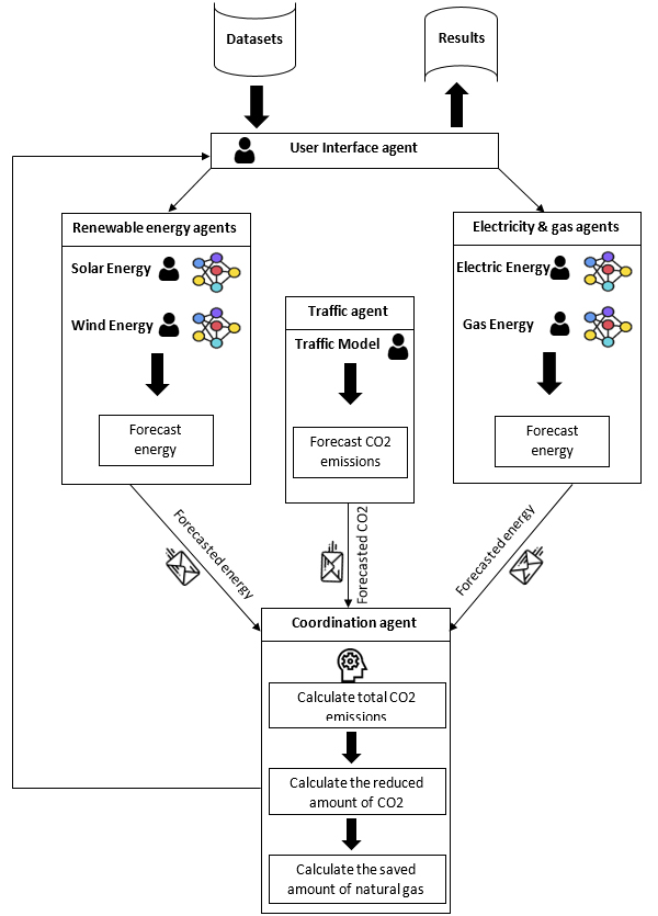

This section describes the system which relies on the power of combining MAS collaborative agents and machine learning forecasting by integrating trained ANN models into autonomous agents. The system consists of multiple forecasting models, each of which is specific to a certain energy type. The agents use the models to forecast the energy production and consumption at each simulation time step. These forecasts are sent to a coordination agent, which calculates the total carbon emissions issued from all available sources and calculates the reduced amount of CO2. The coordination agent also calculates the amount of natural gas saved by using renewable energy.

Figure 1 illustrates the general flow and procedure of the system along with the system’s components, which is composed of different types of agents.

3.2 The prediction models

The first stage focuses on forecasting energy production and consumption. Here, dedicated models are integrated into agents to forecast each type of energy demand. The developed models are MLP artificial neural networks. The networks topologies and parameters were fixed after multiple trials to choose the best topology in terms of the best validation error. The topology and parameters of the models are as follows.

Gas and electricity consumption models: In order to forecast gas consumption and electricity production we used two 3-layer MLP; each MLP is dedicated to one of the two tasks. After several training and validation trials, a hidden layer containing 14 neurons was selected along with a backpropagation optimization algorithm. In order to train each model, the available datasets are divided into training sets and test sets. The training sets are used to adjust the weights and the biases of the networks and the test sets are used for validation in order to ensure better generalization. The next step is the selection of an appropriate input vector to construct the network topology and to construct the training database. In this case, a 10-dimension vector consisting of past energy consumption and temperature values was constructed. The predicted energy load $E$ at hour $t$ is therefore explained by the following previous values: $E_{t-1},E_{t-2},E_{t-3},E_{t-24}$ and $E_{t-168}$ , which represents respectively the load in the previous three hours, the previous day and the previous week’s load at the same hour of the day. In addition to the past load values, the temperature estimations $T$ at the same selected times, i.e. $T_{t-1},T_{t-2,}T_{t-3},T_{t-24}$ and $T_{t-168}$ is used (see Fig. 2).

Figure 2.

The proposed MLP architecture.

The solar energy model: Photovoltaic (PV) energy production depends on multiple factors, for instance, the type of PV module, the degradation of the PV module, solar radiation, and temperature, etc. [51]. In the case of Adrar’s power plant, and in order to forecast the hourly solar energy production, a time series dataset from SONALGAZ was used. The dataset contained 16 months of hourly production in addition to the most influencing factors. The corresponding available exogenous inputs are:

Irradiance, as variation in solar radiation affects many of the PV parameters.

Weather temperature, as the PV module is very sensitive to this aspect. The optimum temperature is 25 ${}^{\circ}$ and generally, the module loses 0.5% of its efficiency per degree increase in temperature.

Wind speed, which can affect the temperature of the PV panel and the irradiance.

The energy production of the previous hour.

In order to forecast the hourly solar energy production, the first 12 months are used to train the model and the next 4 months are used for validation. We fed the neural network an input vector that consists of four parameters, the irradiance, the temperature, the wind speed, and the previous hour’s production value, hence, the solar energy $E$ at the hour $t$ is explained by $Ir_{t-1}$ , $\textit{Temp}_{t-1}$ , ${WS}_{t-1}$ and $E_{t-1}$ .

The wind energy production model: We used a MLP that consists of four neurons in the hidden layer, along with a time series dataset provided by SONALGAZ. The data contains the hourly energy production in addition to the wind speed. To forecast the energy $E$ at the hour $t$ we fed the network two variables, $E_{t-1}$ and ${WS}_{t-1}$ which represent the energy production at hour $t-1$ and the wind speed, respectively. Figure 3 illustrates the architecture of the solar and wind energy models.

The models were trained using the gradient descent algorithm, which is an optimization algorithm used to minimize the cost function by updating the weights of the neural network. Furthermore a hyperbolic tangent (tanh) function was used as an activation function for our models. Table 4 summarizes the used inputs and parameters of the four forecasting models [57].

Table 4

The components of the system

Models	Hidden layer size	Number of inputs	Inputs	Learning rate	Activation function
Electric load	14	10	Previous load and temperature data	0.001	Tanh
Gas consumption	14	10	Previous load and temperature data	0.001	Tanh
Solar energy	8	4	Previous load, irradiance, temperature, wind speed	0.001	Tanh
Wind energy	8	2	Previous load, wind speed	0.001	Tanh

Figure 3.

The renewable energy models.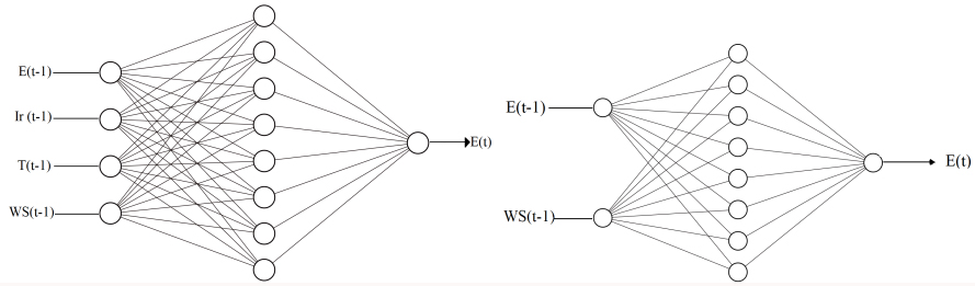

Road traffic CO2 emission model: Traffic emissions are a major source of air pollution, and so to add more depth to our simulator we model traffic emissions. However, due to the lack of datasets and the difficulty of gathering traffic related data, we used a mathematical model based on Eq. (1) and the emission factors in [52]. This model gives an estimation of the CO2 emitted by road traffic at each hour of the day. The amount of CO2 emissions during rush hours is significantly higher due to the increase in traffic density. Hence, traffic emissions $T E$ at the hour $t$ is calculated as follows:

$\displaystyle TE_{t}=E\times N(|\cos(2\pi({t-8})/24|)$ (1)

where $E$ is the yearly average carbon emissions per vehicle divided by the number of hours per year and $N$ is the estimated number of vehicles in the city of Annaba, which according to the Algerian National Office of Statistics [53] is approximately 200,000 vehicles. Equation (1) can illustrate that the rush hours in Annaba, when there is a peak in traffic emissions, occur at 8 am and 8 pm.

3.3 The MAS architecture

Considering that our work focuses mainly on short-term forecasting, we used ANN models as the ANN proved to be an effective technique for forecasting problems, and since we deal with multiple subproblems i.e. forecasting multiple energy sources, calculating the carbon emissions, and investigating the effects of renewable energy, we integrated the ANN in a MAS architecture, as it is known that MAS architecture is a convenient solution for complex or distributed problems, by assigning each subproblem to a distinct autonomous agent. Another advantage of using such approach is the flexibility it offers, to cope with further added functionalities, such as adding more energy and CO2 sources.

The proposed architecture incorporates multiple autonomous agents. There are two types of agents. Firstly, forecasting agents, which are responsible for forecasting energy production and consumption. Secondly, core agents that perform other basic tasks for the simulation, e.g. loading the data, starting the simulation, and displaying the results. The system’s agents are as follows:

•
Gas agent: uses an ANN model to forecast the hourly gas consumption.
•
Electricity agent: uses an ANN model to forecast the hourly electricity production and calculate the equivalent required amount of natural gas to produce such a load.
•
Renewable energy agents (solar and wind agents): use ANN models to forecast the hourly renewable energy production.
•
Traffic agent: uses a mathematical model to calculate the hourly estimated values of traffic emissions.
•
UI Agent: the user interface agent performs some basic yet essential tasks for the simulation, for instance importing data, starting and stopping the simulation, and displaying the results.
•
Coordination agent: the central agent in our architecture. The agent receives the forecasted values from the forecasting agents and calculates the equivalent carbon emissions from each source. These are then summed to obtain the hourly total emitted CO2. The agent then computes the effects of using renewable energies in terms of decreasing air pollution and economizing on the use of natural gas.

Figure 4 illustrates a UML class diagram that describes our system’s agents and their architecture, all the agents are inherited from the principal Agent class, and each agent has its own functionalities, while Fig. 5 illustrates the sequence diagram.

Figure 4.
Class diagram that describes the system agents.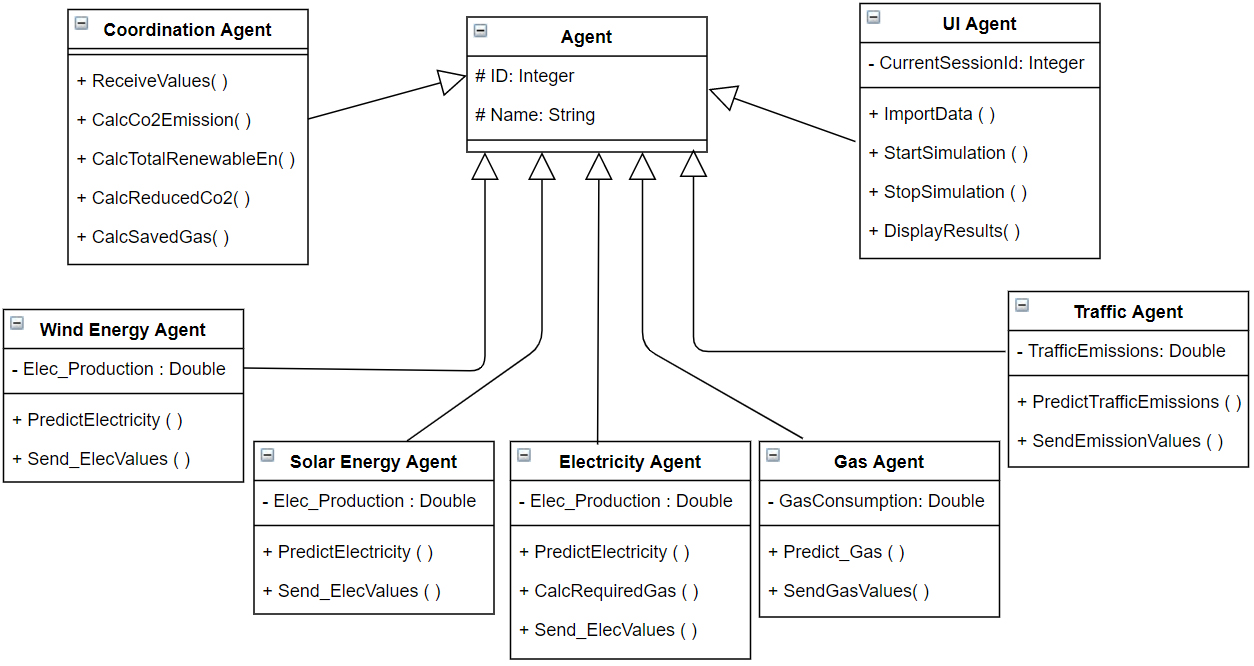

Figure 5.
The system’s sequence diagram.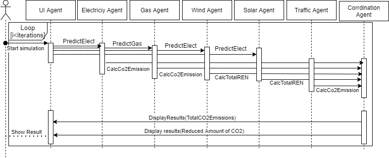

Distributed problem solving is one of the advantages of an agent-based approach. However, it requires cooperation and communications between the agents. The main way of communicating is to exchange messages using an Agent Communication Language (ACL). An ACL allows agents to communicate and share their knowledge in order to reach a goal or solve a problem.

In our system, the agents coordinate among themselves by exchanging messages according to the ACL standard. For instance, the forecasting agents use the ANN models (described in Section 3.2) and share the forecasted energy load with the coordination agent using ACL messages.
4. Simulation results

The overall system is implemented as a simulation tool using the approach described in the above steps. JADE (Java Agent DEvelopment Framework) [54] was chosen to implement the MAS architecture. JADE is an open-source framework written in Java that follows the FIPA (Foundation for Intelligent Physical Agents) specifications and allows the agents to communicate through the ACL Standard. The JADE application consists of one or more containers, and a set of containers composes a platform. Every platform must include a special container called main container which is different from the rest of the containers. The main container includes two special agents: an AMS (Agent Management System) and a DF (Directory Facilitator). The AMS provides the naming service to provide each agent with a unique ID, while the DF enables agents to search and find the agents that provide the service they desire.

The Encog [55] framework, which is a machine learning framework for the .Net and Java programming languages and supports different algorithms, was used to implement the ANN models. The simulation was implemented and tested on a computer with an Intel core i5-6200U CPU 2.40 GHz, with 8 GB of RAM.

4.1 Available data and context

The data used for the work is provided by the national energy distribution company SONALGAZ. More precisely, the electricity dataset covers two years concerning the city of Annaba in Algeria, from 01/01/2014 to 31/12/2015 with a total of 17544 data points.

Hourly temperature estimations were provided by the Algerian meteorological office using the method described in [50]. These estimations use the daily minimum $T_{\textit{mini}}$ and maximum $T_{\textit{maxi}}$ temperatures and are calculated using two equations. The first one assumes that the temperature after sunrise follows a sine curve as follows.

$\displaystyle T_{ih}=({T_{\textit{maxi}}-T_{\textit{mini}}}).\sin\left({\frac{% \pi.t_{a}}{DL_{i}+4}}\right)+T_{\textit{mini}}$ (2)

where $T_{ih}$ is temperature at hour $h$ and $T_{\textit{maxi}}$ and $T_{\textit{mini}}$ are the maximum and minimum temperature at day $i$ , ${DL}_{i}$ is the number of hours from sunrise to sunset, and ta is the counted hours from the sunrise. Secondly, the temperature after sunset is calculated using Eq. (3) assuming that it follows a logarithmic decline:

$\displaystyle T_{ih}=T_{s}-\frac{T_{s}-T_{\textit{mini}+1}}{\ln({24-DL_{i}})}.% \ln({t_{b}})$ (3)

where $T_{s}$ is the temperature at sunset obtained from the case after sunrise using Eq. (1), and $T_{\textit{mini}+1}$ is the minimum temperature of the following day $i+1$ , which is replaced by the minimum temperature of the same day for the times before sunrise. Time $t_{b}$ indicates the time in hours after sunset plus 1 hour.

In addition to the electricity production dataset, the other energy source that is taken into account is natural gas. The hourly natural gas consumption data of the city of Annaba for two main sectors, (residential and the industrial) was provided by SONALGAZ. The dataset covers one year of observations with a total of 8760 data points.

Since the city of Annaba currently does not use renewable energy power plants or sources, the only feasible way to investigate their effects on reducing pollution is through simulation using the case of Adrar city. Adrar city in the south of Algeria obtains 50% of its energy from renewable sources, mainly solar and wind power plants. These are modelled and used as a complementary renewable energy source in the region of Annaba. Adrar’s dataset, used for modelling, contains hourly produced electric load, using wind and solar energy for 2016 and the first half of 2017. Besides the produced load data, the dataset contains other essential exogenous variables for renewable energy production, such as temperature, wind speed, etc.

In order to be able to use the data for machine learning and Neural Network training, it is normalized. Data outputs and inputs are normalized between [0, 1]. Thus, a value of $x$ is normalized to $x^{\prime}$ using the following formula:

$\displaystyle x^{\prime}=\frac{x}{\textit{Xmax}}$ (4)

where $x$ is the old value, $x^{\prime}$ is the new normalized value, and Xmax is the maximum variable value for the year.

Table 5

ANNs performance (RMSE)

Model	Training	Validation
Gas consumption	0.05	0.06
Electricity production	0.04	0.05
Solar energy	0.04	0.11
Wind energy	0.03	0.04

Figure 6.

Comparison between the observed and predicted values for 24 h winter samples for (a) electricity model (b) gas model (c) solar model (d) wind model.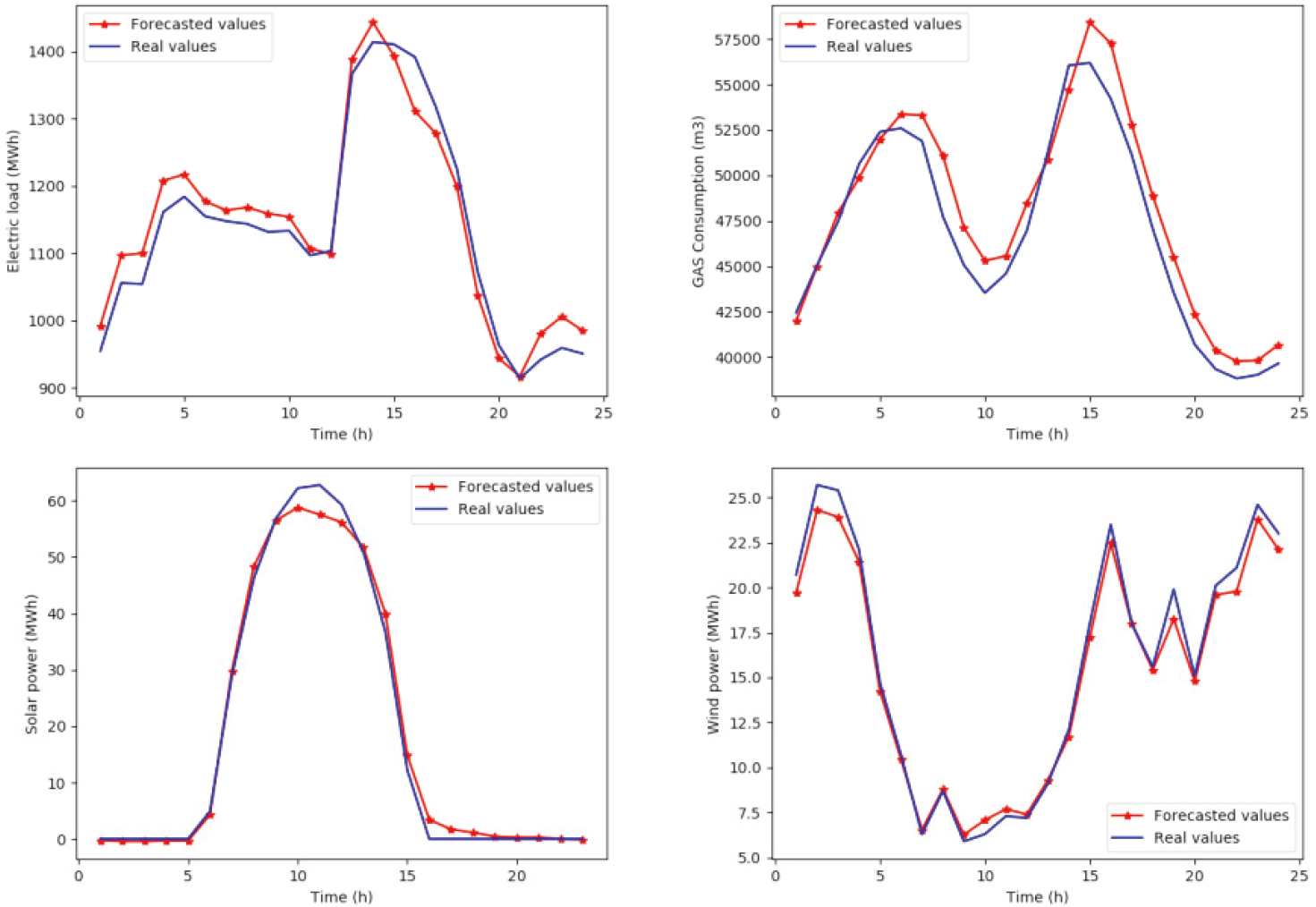

4.2 Experiments

The first simulation stage is the forecasting phase, where the values of energy production and consumption are predicted using the ANN models. In order to test the performance of each model we applied RMSE metric, which is one of the most frequently used evaluation measures. RMSE is computed using Eq. (5) where $a_{l}$ is the predicted value, $b_{l}$ is the observed value, and $l$ is the length of the input vector.

$\displaystyle\textit{RMSE}=\sqrt{\frac{1}{{L}}\sum_{l}^{L}({{a}_{l}-{b}_{l}})^% {2}}$ (5)

After the training phase, the models are then validated using the validation datasets that were not used during training to compute the accuracy of the predictions. Although the ANNs could achieve good performances during the training phase but don’t achieve the same performances on the validation dataset and lose its generalization ability due to over fitting. Therefore, multiple tests with different topologies and configurations were performed in order to choose the best topology in terms of the validation error. Table 5 presents the obtained performances of the four models according to RMSE metric.

Figure 7.

Comparison between the observed and predicted values for 24 h summer samples for (a) electricity model (b) gas model (c) solar model (d) wind model.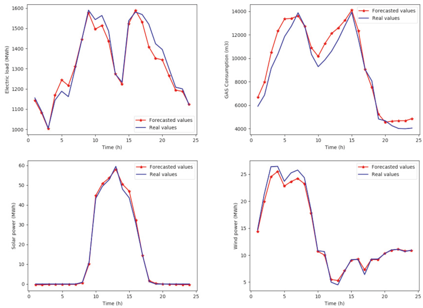

Figure 6 illustrates 24 hours’ prediction samples for each model for winter season. It shows a high similarity between the forecasted and the real consumption values.

Figure 7 shows the results of forecasted and real values for each model for 24 h summer samples. It can be seen that the models are able to give satisfying results in terms of predicting consumption trends. Based on Figs 6 and 7, we can notice that the consumed electricity load during summer is significantly increased, mainly due to the use of air conditioning while the high consumption of natural gas in winter is due to cold weather which forces consumers to use gas-based heating systems.

Since the forecasting phase plays a major role, choosing the best or most efficient model is crucial. Some of the most popular forecasting techniques in the literature, e.g., ARIMA (Auto Regressive Integrated Moving Average) and SVR (Support Vector Regression) were used as benchmarks and their results were compared to the ones obtained by the ANN based SMA Architecture.

ARIMA is a statistical analysis model used in analysing time series data or forecasting future trends. ARIMA models are defined by three main parameters: p the lag size d the degree of differencing, and q the size of the moving average window.

SVR is a machine learning algorithm, and the regression variant of the traditional SVM model SVR maintains all of the main characteristics of SVM such as the use of kernels and the approximation of data points using a hyperplane.

Both of the models are fed with the same training and test data as the ANN models and the same RMSE metric is used to compare their performances. Table 6 presents the results and demonstrates that the ANN models achieved better performances than the ARIMA and SVR models.

Table 6

The performance of the models (RMSE)

Model	ANN	SVR	ARIMA
Gas consumption	0.06	0.21	0.07
Electricity production	0.05	0.36	0.09
Solar energy	0.11	0.38	0.22
Wind energy	0.04	0.33	0.21

Figure 8.

The CO2 emission issued from electricity generation (a) in winter (b) in summer.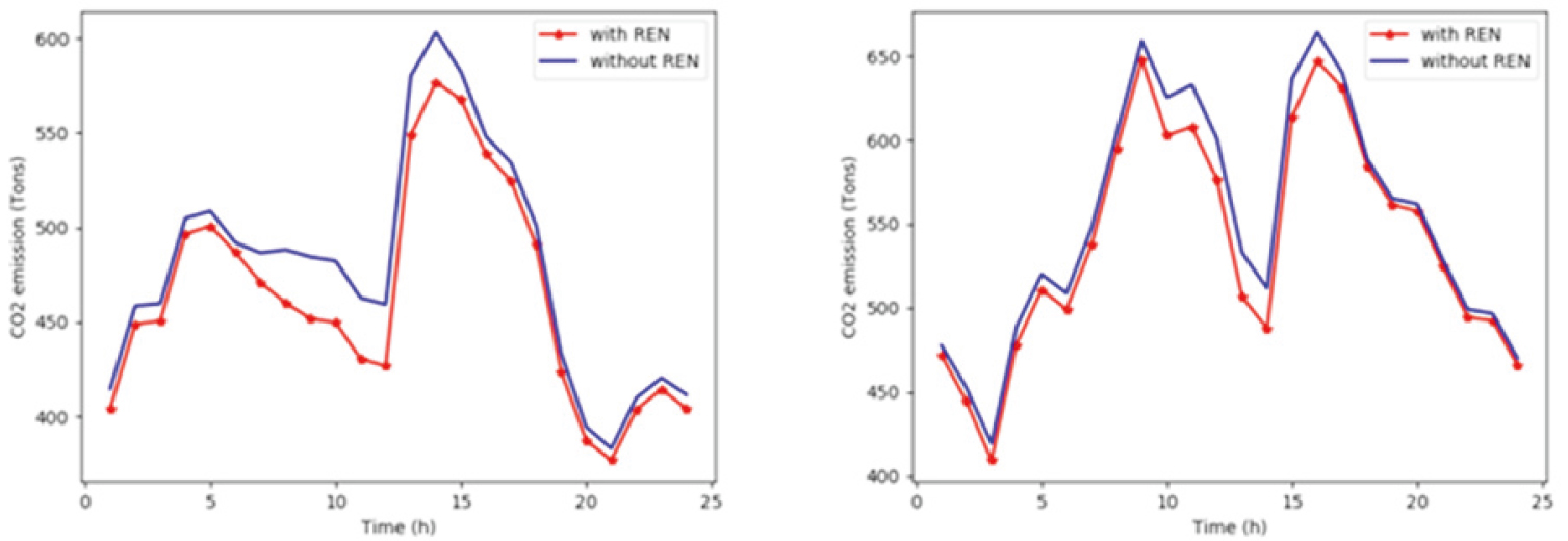

For each hourly simulation step, forecasting agents predict energy production and consumption and communicate their values to the coordination agent. The latter has two main tasks. The first is to calculate the equivalent amount of burned natural gas that was used to produce the forecasted electricity production. This is computed according to the U.S Energy Information Administration [56] by Eq. (6).

$\displaystyle AG=HR/HV$ (6)

where AG is the amount of gas used per kWh, HR is the heat rate of the power plant and HV is the heat value of the used fuel. Hence, the amount of natural gas needed to generate one kWh is 0.00786 Mcf which is equivalent to 0.22 m ${}^{3}$ . This assumes that the average HR of a natural gas-fired power plant is 8,039 Btu/kWh and the HV of natural gas is 1,023,000 Btu/Mcf.

The second task is to calculate the environmental cost of the produced energy. The agent computes the equivalent carbon emissions in the forecasted hour according to the emissions of natural gas in [52]. This indicates that the CO2 equivalent of burning natural gas is 0.0551 metric tons CO2/Mcf which is equal to 0.0019 metric tons CO2/m ${}^{3}$ . Finally, to simulate the benefits of using cleaner energy sources, the agent calculates the effects of using renewable energies on air pollution, i.e. the reduced amount of carbon emissions and the amount of fossil energy that would be saved.

Figure 8 shows a comparison between the carbon emissions coming from electricity generation using natural gas, and carbon emissions using renewable energies (REN) to generate a portion of the load. The results show the benefits of using renewable energies as an alternative solution to generate electric power. According to the simulations, using solar and wind energy can help reduce the emissions by a maximum of 33 tons of CO2 per hour, with an average of 15 tons of CO2 per hour.

Since producing electricity consumes a large amount of natural gas, using renewable energies can considerably reduce the amount of gas used. Based on the previous two samples shown in Fig. 8, Tables 7 and 8 highlight some simulation results and statistics.

Table 7

Comparison between the obtained CO2 emissions from electricity generation (in Tons)

Sample	MAX hourly emissions	MIN hourly emissions	AVG hourly emissions	Daily emissions
Winter without REN	603	383	479	11505
Winter with REN	576	377	464	11136
Summer without REN	664	419	551	13232
Summer with REN	647	409	539	12948

Table 8

Comparison between the simulated amount of natural gas (NG) usage for electricity generation (in m3)

Sample	MAX hourly burned NG	MIN hourly burned NG	AVG hourly burned NG	Daily burned NG
Winter without REN	317640	201740	252303	6055280
Winter with REN	303600	198440	244227	5861460
Summer without REN	349580	220660	290189	6964540
Summer with REN	341000	215380	283955	6814940

To calculate the total carbon emissions, the coordination agent sums the emission values from all of the models simulation results. Hence, the CO2 emission at hour $t$ is explained by as follows:

$\displaystyle CO2_{t}=GE_{t}+EE_{t}+TE_{t}$ (7)

where ${GE}_{t}$ , ${EE}_{t}$ , $TE_{t}$ , represent the gas consumption, electricity production, and the traffic emissions respectively at hour $t$ . Although CO ${}_{2}$ emissions in the residential sector may depend on multiple factors, in this work we only consider that it is equal to the emissions from natural gas and natural gas burned to produce electric power. Figure 9 illustrates the results obtained from a simulation of the total carbon emissions on a typical winter day.

Figure 9.

Total CO2 emission.

5. Conclusions and future work

The state-of-the-art techniques have proved to be efficient in forecasting CO2 emissions and solving distributed problems. However, these works suffer from some limitations, for instance, they focus only on forecasting CO2 emissions and do not address the problem of forecasting the energy source that is responsible for these emissions. The presented work aimed to fill this gap by jointly forecasting the type of energy source and their equivalent CO2 emissions. Moreover, another problem that has not been addressed is CO2 emission reduction policies. Therefore, in this paper, how renewable energy can be used to reduce energy related CO2 and fossil energy consumption is examined. The contribution consists of a collaborative MAS for forecasting hourly CO2 emissions issued from energy consumption and production, where multiple ANN forecasting models are embedded in various forecasting agents and each model was trained to forecast a specific type of energy; in addition, a mathematical model was used to estimate traffic emissions. The results are promising, as the system was able to achieve satisfying prediction performances, and was able to give some estimations of the benefits of using renewable energies. Therefore, the work has demonstrated that an agent-based approach can be a suitable solution to model complex problems and, in particular pollution-related issues and energy management systems.

For future work, we aim to improve our simulator by enhancing the precision of the ANN models to obtain better forecasting. We will also extend the simulator to include production sources of other greenhouse gases and include more sources of energy and air pollution, such as industrial activities.

Footnotes

Acknowledgments

This work is funded by the Directorate General for Scientific Research and Technological Development (DGRSDT).

Author’s Bios

Seif Eddine Bouziane is a Ph.D. Student at the Department of Computer Science of the University of Badji Mokhtar Annaba in Algeria. He got his master degree in computer science (Information and Communication Systems and Technologies) in 2017 from the University of Badji Mokhtar. His areas of interest and research include machine learning and agent-based systems.

Mohamed Tarek Khadir graduated from the University of Badji Mokhtar Annaba, Algeria, with a state Engineering degree in Electronics Majoring in Control, in 1995. After two years’ work in the computer industry, he undertook an M.Eng. at Dublin City University, Ireland Graduating with First class honors in 1998. Tarek Khadir received a Ph.D. degree from the National University of Ireland, Maynooth, Ireland in 2002. He then continued with this institution as a post-doctoral researcher until September 2003 when he joined the department of computer science at his university of origin, university Badji Mokhtar Annaba, Algeria, as a senior lecturer. He succeeded in obtaining the HDR (Habilitation to Direct Research) in January 2005 and got promoted to full professor in 2010.

Julie Dugdale is the leader of the HAwAI research team and an Associate Professor at the University Grenoble Alps in France. She received her Ph.D. from the University of Buckingham, England in 1994 in the area of artificial intelligence. Before coming to France, she was an associate professor at the University of Montfort, England. In 2013 she received her HDR (Habilitation to Direct Research) from University Joseph Fourier, Grenoble. Her research interest focuses on cognition and interaction. Specifically, modeling the cognitive activities of human behavior. Generally, her work falls into the domain of Agentbased Social Simulation (ABSS).

References

www.who.int/health-topics/air-pollution. Last accessed: 27/06/2020.

www.energy.gov.dz/Media/galerie/benational2018-edition-20195dac85774bce1.pdf. Last accessed: 04/03/2020.

Khraief

Shahbaz

Mallick

and Loganathan

, Estimation of electricity demand function for Algeria: revisit of time series analysis, Renewable and Sustainable Energy Reviews 82 (2018), 4221–4234.

Bouraiou

Necaibia

Boutasseta

Mekhilef

Dabou

Ziane

Sahouane

Attoui

Mostefaoui

and Touaba

, Status of renewable energy potential and utilization in Algeria, Journal of Cleaner Production 246 (2016).

Kizilaslan

and Karlik

, Comparison Neural Networks Models for Short Term Forecasting of Natural Gas Consumption in Istanbul, in: 2008 First International Conference on the Applications of Digital Information and Web Technologies (ICADIWT), Ostrava, 2008, pp. 448–453.

Suykens

Lemmerljng

P.H.

Favoreel

Crepe

and Briol

, Modelling the Belgian gas consumption using neural networks, Neural Processing Letters 4 (1996), 157–166.

Laib

Khadir

M.T.

and Chouired

, Forecasting yearly natural gas consumption using Artificial Neural Network for the Algerian Market, in: 2016 4th International Conference on Control Engineering & Information Technology (CEIT), Hammamet, Tunisia, (2016), pp. 1–5.

Hsu

Y.Y.

Tung

T.T.

Yeh

H.C.

and Lu

C.N.

, Two-stage artificial neural network model for short-term load forecasting, IFAC-PapersOnLine 51 (2018), 678–683.

Jetcheva

J.G.

Majidpour

and Chen

W.P.

, Neural network model ensembles for building-level electricity load forecasts, Energy and Buildings 84 (2014), 214–223.

10.

Chen

Qiao

and Lu

, Probabilistic short-term wind power forecasting based on deep neural networks, in: International Conference on Probabilistic Methods Applied to Power Systems (PMAPS), Beijing, China, 2016.

11.

Peng

Xiong

Wen

Fan

Feng

and Wang

, A very short term wind power prediction approach based on Multilayer Restricted Boltzmann Machine, in: IEEE PES Asia-Pacific Power and Energy Engineering Conference (APPEEC), Xian, China, 2016.

12.

Bhaskar

and Singh

S.N.

, AWNN-assisted wind power forecasting using feed-forward neural network, IEEE Transactions on Sustainable Energy 3 (2012), 306–315.

13.

Marugan

Marquez

Perez

and Hernandez

, A survey of artificial neural network in wind energy systems, Applied Energy 228 (2018), 1822–1836.

14.

Zhong

Liu

Sun

and Wang

, Prediction of photovoltaic power generation based on general regression and back propagation neural network, Energy Procedia 152 (2018), 1224–1229.

15.

Abuella

and Chowdhury

, Solar Power Forecasting Using Artificial Neural Networks, North American Power Symposium (NAPS), Charlotte, USA, 2015.

16.

Wang

and Song

, A deep spatial-temporal ensemble model for air quality prediction, Neurocomputing 314 (2018), 198–206.

17.

Zhou

Zhao

Lin

Wang

and Li

, A Gaussian process mixture model-based hard-cut iterative learning algorithm for air quality prediction, Applied Soft Computing 58 (2019).

18.

Athira

Geetha

Vinayakumar

and Soman

K.P.

, DeepAirNet: applying recurrent networks for air quality prediction, Procedia Computer Science 132 (2018), 1394–1403.

19.

Maciag

P.S.

Kasabov

Kryszkiewicz

and Bembenik

, Air pollution prediction with clustering-based ensemble of evolving spiking neural networks and a case study for London area, Environmental Modelling & Software 118 (2019), 262–280.

20.

Moustris

K.P.

Larissi

I.K.

Nastos

P.T.

and Koukoulestos

, Development and application of artificial neural network modeling in forecasting PM10 levels in a Mediterranean City, Water, Air, and Soil Pollution 224 (2013).

21.

Azid

Juahir

Toriman

Kamarudin

Saudi

Hasnam

Aziz

Azaman

Latif

Zainuddin

Osman

and Yamin

, Prediction of the level of air pollution using principal component analysis and artificial neural network techniques: a case study in Malaysia, Water, Air, and Soil Pollution 225 (2014).

22.

and Lin

, A novel optimal-hybrid model for daily air quality index prediction considering air pollutant factors, Science of the Total Environment 683 (2019), 808–821.

23.

Lin

Lee

Ouyang

and Wu

, Air quality prediction by neuro-fuzzy modeling approach, Applied Soft Computing 86 (2020).

24.

Cheng

Ding

Lin

and Xu

, Air quality prediction at new stations using spatially transferred bidirectional long short-term memory network, Science of the Total Environment 705 (2020).

25.

Wang

and Zhang

, Research on carbon emissions and its trend forecast of Baoding, in: Sixth International Conference on Advanced Computational Intelligence (ICACI), Hangzhou, China, 2013, pp. 39–44.

26.

Lau

E.T.

Yang

Forbes

A.B.

Wright

and Livina

V.N.

, Modelling carbon emissions in electric systems, Energy Conversion and Management 80 (2014), 573–581.

27.

Sheta

A.F.

Ghatasheh

and Faris

, Forecasting Global Carbon Dioxide Emission Using Auto-Regressive with eXogenous Input and Evolutionary Product Unit Neural Network Models, in: 2015 6th International Conference on Information and Communication Systems (ICICS), Amman, Jordan, 2015, pp. 182–187.

28.

Wang

Z.X.

and Ye

D.J.

, Forecasting Chinese carbon emissions from fossil energy consumption using non-linear grey multivariable models, Journal of Cleaner Production 142 (2017), 600–612.

29.

Lin

Guan

and Lin

, The prediction of carbon emission in all provinces of China with the K-means cluster based Logistic model, in: 2017 International Conference on Service Systems and Service Management, Dalian, 2017, pp. 1–6.

30.

Ding

Dang

Y.G.

X.M.

Wang

J.J.

and Zhao

, Forecasting Chinese CO2 emissions from fuel combustion using a novel grey multivariable model, Journal of Cleaner Production 162 (2017), 1527–1538.

31.

Fang

Zhang

Jin

T.C.

and Tian

, A novel method for carbon dioxide emission forecasting based on improved Gaussian processes regression, Journal of Cleaner Production 173 (2018), 143–150.

32.

Mason

Duggan

and Howley

, Forecasting energy demand, wind generation and carbon dioxide emissions in Ireland using evolutionary neural networks, Energy 155 (2018), 705–720.

33.

Hong

Jeong

and Koo

, An optimized gene expression programming model for forecasting the national CO2 emissions in 2030 using the metaheuristic algorithms, Applied Energy 228 (2018), 808–820.

34.

Huang

Shen

and Liu

, Grey relational analysis, principal component analysis and forecasting of carbon emissions based on long short-term memory in China, Journal of Cleaner Production 209 (2019), 415–423.

35.

Safdarnejed

S.M.

Tuttle

J.F.

and Powell

K.M.

, Dynamic modeling and optimization of a coal-fired utility boiler to forecast and minimize NOx and CO emissions simultaneously, Computers & Chemical Engineering 124 (2019), 62–79.

36.

Ding

Gong

and Bai

, Forecasting Chinese greenhouse gas emissions from energy consumption using a novel grey rolling model, Energy 175 (2019), 218–227.

37.

Sangeetha

and Amudha

, A novel bio-inspired framework for CO2 emission forecast in India, Procedia Computer Science 125 (2018), 367–375.

38.

Wooldridge

and Jennings

N.R.

, Intelligent agents: theory and practice, The Knowledge Engineering Review 10 (1995), 115–152.

39.

Russell

S.J.

and Norvig

, Artificial Intelligence “A modern approach”, Prentice-Hall, Volume 25, 1995.

40.

Aulinas

Turon

and Sànchez-Marrè

, Agents as a Decision Support Tool in Environmental Processes: The State of the Art, Whitestein Series in Software Agent Technologies and Autonomic Computing, 2009, 5–35.

41.

Ghazi

Dugdale

and Khadir

M.T.

, Modelling Air Pollution Crises Using Multi-Agent Simulation, in: 49th Hawaii International Conference on System Sciences (HICSS), Koloa, HI, 2016, pp. 172–177.

42.

Dragomir

E.G.

and Oprea

, A multi-agent system for power plants air pollution monitoring, IFAC Proceedings Volumes 46 (2013), 89–94.

43.

El Fazziki

Benslimane

Sadiq

Ouarzazi

and Sadgal

, An agent based traffic regulation system for the roadside air quality control, in IEEE Access 5 (2017), 13192–13201.

44.

Corchado

M.J.

Mata

and Rodriguez

, A Multi-Agent System for Modeling and Monitoring the Evolution of Oil Slicks in Open Oceans, Advanced Agent-Based Environmental Management Systems, Basel, 2009, 91–117.

45.

Di Lecce

Amato

Martines

di Bari

and Dario

, Air quality control for health care centres, The application of an intelligent distributed system, IEEE Workshop Environmental, Energy, and Structural Monitoring Systems, 2009.

46.

Papaleonidas

and Iliadis

, Hybrid and reinforcement multi agent technology for real time air pollution monitoring. Artificial Intelligence Applications and Innovations 381 (2012), 274–284.

47.

Ahat

Ben Amor

Bui

Lamure

and Courel

, Pollution modeling and simulation with multi-agent and pretopology, lecture notes of the institute for computer sciences, Social Informatics and Telecommunications Engineering 4 (2009), 225–231.

48.

El Fazziki

Sadiq

Ouarzazi

and Sadgal

, A Multi-Agent Framework for a Hadoop Based Air Quality Decision Support System, in: Conference on Advanced Information Systems Engineering, Stockholm, Sweden, 2015.

49.

Hulsmann

Gerike

and Ketzel

, Modelling traffic and air pollution in an integrated approach – the case of Munich, Urban Climate 10 (2014), 732–744.

50.

Farfar

K.E.

and Khadir

M.T.

, A two-stage short-term load forecasting approach using temperature daily profiles estimation, Neural Computing and Applications 31 (2018).

51.

Vidyanandan

K.V.

, An overview of factors affecting the performance of solar PV systems, Energy Scan 27 (2017), 2–8.

52.

www.epa.gov/energy/greenhouse-gases-equivalencies-calculator-calculations-and-references. last accessed: 2020/03/26.

53.

www.ons.dz/. Last accessed: 30/03/2020.

54.

Bellifemine

Poggi

and Rimassa

, JADE – a FIPA-compliant agent framework, Jade 99 (1999), 3.

55.

Heaton

, Encog: Library of Interchangeable Machine Learning Models for Java and C#.

56.

https://www.eia.gov/tools/faqs/. Last accessed: 01/04/2020.

57.

Hao

, A gradient descent method for solving a system of nonlinear equations, Applied Mathematics Letters (112) (2011).

A collaborative predictive multi-agent system for forecasting carbon emissions related to energy consumption

Abstract

Keywords

1. Introduction

2. Literature review

2.1 ANN for forecasting energy consumption

Table 1 Summary of ANN energy forecasting papers

Table 2 Summary of energy-related emission papers

3. Methodology

3.1 Overview

Table 3 Summary of MAS pollution related papers

4.1 Available data and context

Footnotes

Acknowledgments

Author’s Bios

References

Table 1
Summary of ANN energy forecasting papers

Table 2
Summary of energy-related emission papers

Table 3
Summary of MAS pollution related papers