
Abstract
Imbalanced data classification (IDC) presents a significant challenge in data mining (DM), as it frequently occurs in various real-world areas with profound implications for highly skewed databases. IDC revolves around the task of learning from data characterized by a substantial imbalance in the number of samples across its different classes. Hence the Polar-CanisFel (PCF) Optimization-deep ensemble model is designed to address imbalanced big data issues, incorporating the SMOTE technique for rebalancing the dataset. This ensemble classifier leverages a deep convolutional neural network (DCNN), Long Short-Term Memory (LSTM), and Gated Recurrent Neural Network (GRNN) architectures for effective data classification. For the Heart Failure Prediction Dataset, the model reaches an accuracy of 96.35%, sensitivity of 94.54%, and specificity of 96.11%. Further, the accuracy of 95.91%, sensitivity of 95.87%, and specificity of 94.79% are obtained concerning the Stroke Prediction dataset. Finally, when applied to the Hepatitis-C prediction dataset, the model attains an accuracy of 92.79%, sensitivity of 92.90%, and specificity of 92.63% during 90% of training.
Keywords
Introduction
In recent times, a variety of strategies have emerged to tackle the challenges posed by unbalanced data. These strategies can be categorized into four major groups. First, we have data-level approaches, which do not rely on a specific classifier but rather focus on preprocessing the input data before constructing a discrimination function [13]. These approaches often involve techniques such as resampling and feature selection/extraction. Resampling techniques, which involve actions like removing instances or generating artificial examples, are employed to balance the class distribution in the dataset [7,17]. One notable approach in this category involves dividing the majority class into subsets, each of which matches the size of the minority class. Ensemble methods are then used to train various learning algorithms on these subsets, often yielding competitive performance [18,20]. Another group of strategies falls under the category of cost-sensitive methods. These techniques modify the learning algorithm to penalize incorrect classification of the minority class, with the “Cost-sensitive and Hybrid Attribute Measure Multi-Decision Tree” (CHMDT) being a well-known example [13]. Algorithmic-level approaches represent the third category, which involves extensions and variations of traditional classifiers designed to improve imbalanced learning [24]. These approaches address the challenges of imbalanced data classification by enhancing the performance of classifiers. The efficiency of computational classification techniques is significantly impacted by the substantial class imbalances found in real-world datasets [6]. For example, detecting cancer from testing data may involve identifying only a few samples as cancer patients, while the majority are labeled as normal [21]. Similar imbalances are observed in fields such as intrusion detection, fraud identification, and credit loans [2,16,22].
Traditional classification algorithms are often ill-equipped to handle imbalanced data due to their assumption of balanced data distribution, leading to potential inefficiencies [13,24]. In imbalanced datasets, the minority class is typically assigned more significance, as correctly identifying minority events is of utmost importance [6]. For instance, in medical diagnosis, misclassifying a malignant tumor as benign can have life-threatening consequences. As a result, the problem of imbalanced data classification has gained recognition as one of the most challenging issues in the machine learning (ML) and data mining (DM) communities [14]. Methods for processing imbalanced data reduce the dominance of the majority class by emphasizing oversampling or undersampling of the minority or majority class [7]. However, these techniques come with their own set of challenges, such as the need to address overfitting and parameter tuning [7,23]. In response to these challenges, a deep neural network-based algorithm was developed to address the classification of class-imbalanced data, acknowledging the significant influence of data quantity on the performance of convolutional neural networks (CNN) [8]. Algorithm-based techniques, however, have limitations, particularly in addressing ambiguous decision boundaries between minority and majority samples [6]. Overall, addressing the problem of imbalanced data classification requires careful parameter tuning and consideration of data quantity and quality. Enhancing classification accuracy while mitigating overfitting issues can be achieved through strategic adjustments. A training data selection strategy, as outlined in [5], utilizes the roulette wheel selection method. Furthermore, in [15], the generation of kernel-generated surfaces is demonstrated, specifically tailored for nonlinear cases. Moreover, in [4], the utilization of Variational Autoencoders (VAE) to generate implicit variables with a posterior distribution as inputs for Generative Adversarial Networks (GAN) is explored. Additionally, a similarity measure loss is introduced into the generator to enhance the quality of minority class samples generated by the GAN.
The main intention is to develop a model for IDC with a PCF-deep ensemble model, in which the unbalanced data is pulled together from the database and preprocessed to weed out extraneous data. The preprocessed data is fed into SMOTE, where it is balanced out from enormously unbalanced data and aids in the creation of an equivalent number of synthetic data samples. The hunting and feeding characteristics of the Polar Bear Optimization Algorithm (PBO) [9], Coyote Optimization Algorithm (COA) [3], Cat Swarm Optimization (CSO) [1], and Grey Wolf Optimization (GWO) [12] are hybridized to create the PCF optimization method to get the best solution. The primary contribution of the research is as follows;
The following manuscript is organized as: The model’s background information is given in Section 1, as well as the requirements for imbalance data classification are determined in Section 2 through a review of the literature. Section 3 discusses the proposed imbalanced data classification. The analysis of the consequences is integrated in Section 4, and assumptions are enclosed in Section 5.
Literature review
The IDC survey is described below;
A learning model was introduced to balance imbalanced medical data by training sampled data and regulating the hybrid sampling process. However, this approach quickly balances data but exhibits poor classification accuracy [20]. In [8] deep learning focused on increasing the accuracy of classifying minority samples in medical data while maintaining overall accuracy. The method is fast but struggles with significant class differences and similarities between defects. An innovative approach [23] aimed to overcome randomness restrictions in data imbalance classification by addressing arbitrary sampling ratios. This method provides consistent classification performance and is less time-consuming. A hybrid approach [14] was presented for IDC, aiming to select the best majority and minority data for creating new samples and removing unnecessary data. It focuses on density perception, reducing computational complexity but with high time complexity. In [7] machine learning was used to improve minority class instances while reducing the prominence of majority class instances. It achieves quick computation but is susceptible to overfitting. A density-grounded machine learning method was introduced in [6] to enhance prediction accuracy, especially for minority classes. It aimed to minimize misclassification but didn’t address the challenge of determining boundaries between minority classes. In [24] a deep learning-based approach focused on improving the recognition rate of the minority class in imbalanced data, although it required more time and effort for training compared to conventional oversampling methods. An enhanced machine learning strategy aimed to improve classification performance while maintaining high accuracy [13], although it wasn’t suitable for handling large-scale problems and didn’t require complex algorithm tuning. These studies highlight various approaches to addressing imbalanced data classification, each with its strengths and limitations.
The previous studies have several problems, such as overfitting, significant differences within the same class, restrictions on removing the useful majority class samples, similarities between different defects, and significant differences within the same class. Furthermore, the question of where to draw the boundaries between minority classes has not been addressed by cutting-edge methodologies. In this work, these problems are addressed by creating the proposed model to classify the imbalanced data.
Polar-CanisFel optimization-based deep ensemble model for classification of imbalanced data
The key intention of the research is to develop a classification model to handle the unbalanced big data, in which the unbalanced input data is gathered from different databases like the Heart Failure Prediction Dataset,[10], Stroke Prediction dataset [19], and Hepatitis-C prediction dataset [11]. These gathered data are then subjected to the phase of data preprocessing, which is considered as the initial stage for classifying the unbalanced data that eradicates the irrelevant data. The preprocessed data is subjected to the phase of data balancing, in which it comprises the SMOTE to balance the unbalanced data. When the unbalanced data is balanced with SMOTE, then it automatically passes to the stage of feature extraction to extract the features, as well as Euclidean distance-based Graph embedding (ED-based GE) technique is comprised for this extraction process. The extracted data is subjected to the proposed framework such as PCF optimization for handling the incremental data to handle the computational complexity, in which the balanced data is divided as subsets with the master nodes, and then it is again divided as reducer nodes to generate the output node as a final node. Also, it consists of an optimized deep ensemble model, which is developed by combining the features of hunting and feeding through the optimization algorithms [1,3,9,12] that is developed with the DCNN, in which the tuning parameters like bias, as well as weight, is tuned optimally with the proposed optimization to generate the output of classification. Finally, these classified results from the individual master nodes of the proposed architecture are integrated into the individual slave nodes, to create the classified output. The implementation of the developed model is done through the PYTHON tool, as well as the analysis of the developed model depends on performance metrics like precision, recall, as well as accuracy. Figure 1 portrays the schematic representation of the PCF-deep ensemble model for Imbalanced Data Classification.
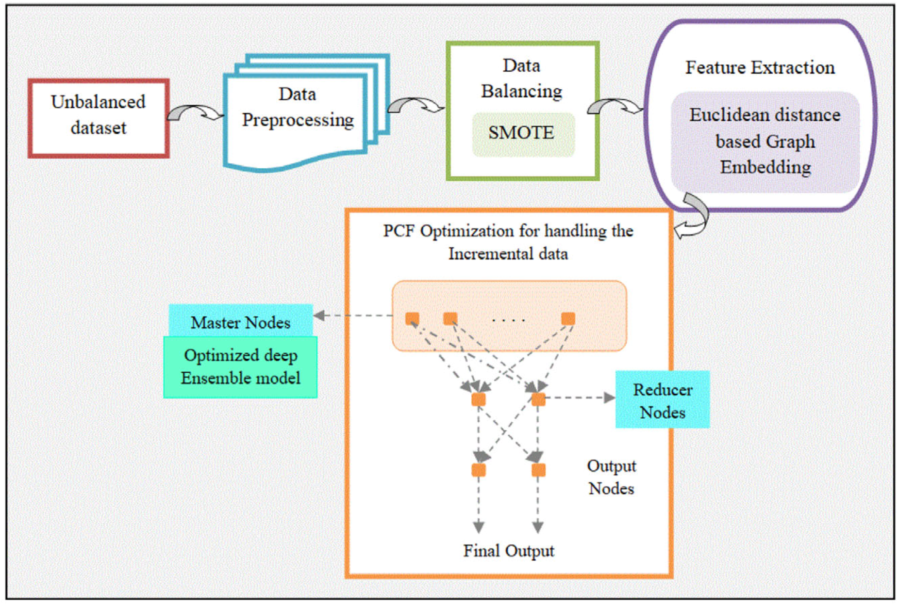
Graphical depiction of the PCF-deep ensemble model.
The unbalanced input data for imbalanced data classification is gathered from three databases Heart Failure Prediction Dataset [10], Stroke Prediction dataset [19], and Hepatitis-C prediction dataset [11]. The input data gathered from the datasets are represented as
Pre-processing unbalanced data
When the input is gathered from three databases such as [10,19], and [11], then it automatically undergoes the phase of pre-processing, which is referred to as the prior stage while classifying the imbalanced data to extract the representative information from the system, as well as construct optimized structures of data
Data balancing with SMOTE architecture
The performance of the processed unbalancing data depending on the database must be balanced to increase the robustness of the ensemble deep classifier regarding accuracy. Therefore, the data imbalance is necessary to obtain the best consequences as well as robustness, which is the major crisis in ML when skilled on imbalanced datasets. Consequently, SMOTE is utilized for managing the issues of data imbalance to get better performance of the deep classifier. To create samples that are balanced with the class majority, synthetic samples are incorporated into the minority samples. The samples are generated by considering the occurrences of feature space in the SMOTE approach.
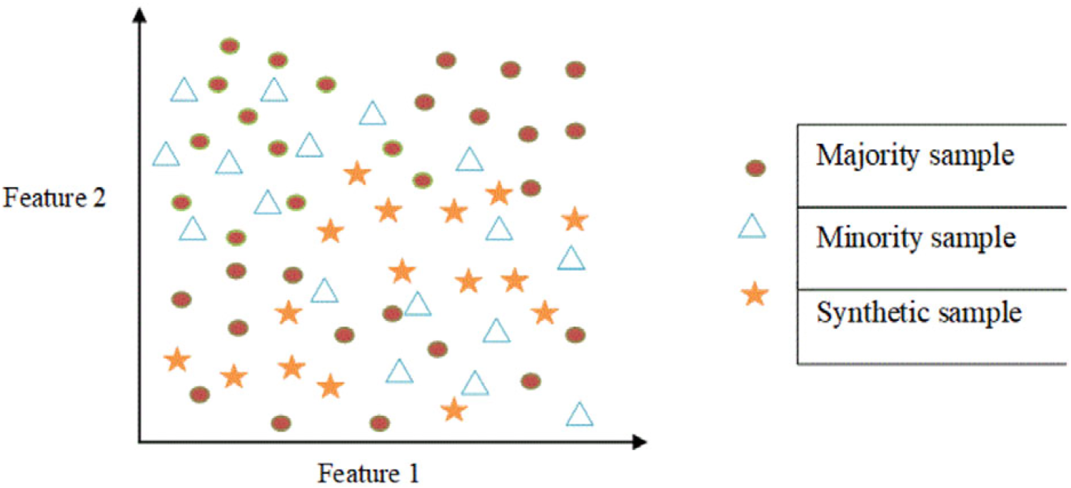
SMOTE architecture.
The sample does not afford the difference in ML even though the sample increases the data quantity. Then, the synthetic information generates between the arbitrary information as well as selects the adjacent neighbor. As a consequence, this SMOTE is employed to balance the imbalanced database. SMOTE is intended to include a new system arbitrarily between minority samples as well as neighbors and works out two cases to generate a synthetic case, which is depicted in Figure 2. In general, SMOTE uses the KNN to generate the synthetic information from the alternative samples with the calculation of distance among incoming as well as accessible samples. The SMOTE is expressed by assigning the sampling enlargement of the database T as;

When the balanced data is divided as subsets with the master nodes, then the developed optimized ensemble classifier is performed for classifying the data. At last, the classified results from the particular master nodes of the developed architecture are integrated into the individual slave nodes to create the final output of classification. When new data arrives, then the error among the predicted output as well as the outputs of expected classification is derived in the testing stage. Subsequently, the selection measure is verified, where the error will be compared with the threshold value of the error in such a way that if the estimated error lies below the preset threshold value, the learned model will be maintained or otherwise, the classifier remodeling will be initiated. The remodeling of the classifier makes sure that update the hyper-parameters of the classifier.
The balanced data is subjected to feature extraction which comprises the ED-based GE technique for extraction. Here, the node embedding (NE), as well as edge embedding (EE) is carried out, in which the node embedding denotes every node as a vector in a space of low dimension, which is “close” in the graph and is embedded to include parallel vector illustration. The variation among several graph embedding techniques lies based on the “closeness” between two nodes.EE intends to characterize an edge as a low-dimensional vector, which is functional in two states. Initially, knowledge graph embedding (K-GE) learns to embed for both nodes as well as edges. Subsequently, some embed a pair of nodes as a vector feature to either create a node pair similar to other nodes or forecast the link continuation among two nodes. The GE based on Matrix factorization signifies the graph property in matrix form and factorizes it to acquire NE and there are two forms of Matrix factorization (MF) such as graph Laplacian eigenmaps, and node proximity matrix. The GE is done based on the Euclidean distance, which is referred to as the distance between two feature vectors such as
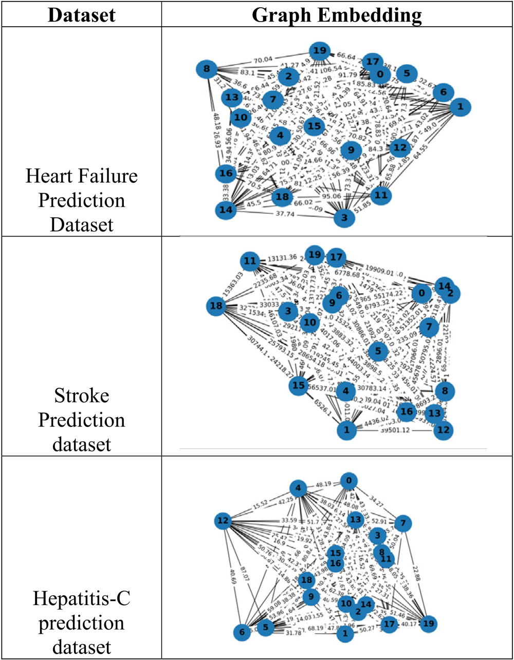
Graph embedding.
Generally, the deep ensemble network is referred to as the popular technique, which functions through retraining similar neural networks several times, as well as averaging the consequently systems that are illustrated in Figure 4. The system combines the merits of both the models of deep and ensemble learning. Thus, the final system possesses better performance. The CNN-LSTM-GRU model provides the effective classification of the extracted local and long-term global data representations. Further, the ensemble model assigns the weighted average of the individual models, and the PDF optimizations are utilized in the model to tune the hyperparameters such as bias as well as weight to attain effective classification.
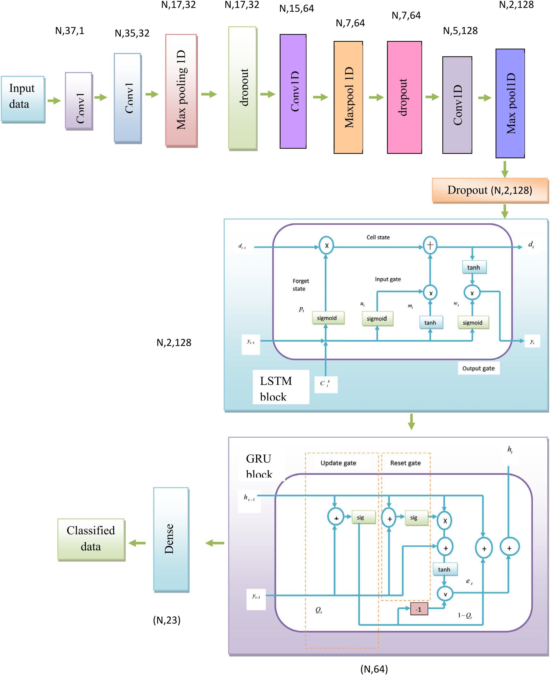
Blockwise representation of the PCF-deep ensemble model.
i
CNN are the neural networks that utilize convolution as a replacement for the general matrix multiplication, in which the model can learn arbitrary yet complex connections without requiring to learn directly from the lag data. As a consequence, CNN learns the multiple series of inputs to determine which representation is most pertinent to the prediction problem. Additionally 1D conv layer operates on sequential data to process the time-series features and minimizes the complexity effectively. The max-pooling enables choosing only the maximum value for obtaining the most distinctive features of the data. Unlike traditional neural networks, CNN utilizes the convolution layers to encode the information. Further the convolutional layer outputs attained by applying the non-linear activation function are formulated as,
LSTM network is an advancement over the RNN, typically consisting of a set of memory blocks arranged in a pattern to form the LSTM cells and mitigate the vanishing gradient issue. LSTM receives the input data with the dimension


Further, the GRU predicts the output with the dimension of
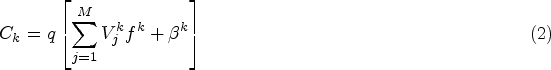
Gated Recurrent Unit is a modified version of LSTM that assists in capturing the dependencies at multiple time scales from the input of


Where
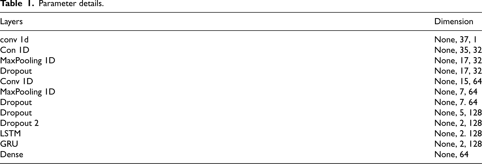
The parameter details of the developed deep ensemble model are depicted in Table 1 and the architecture of the PCF-deep ensemble model is portrayed in Figure 5.
Parameter details.
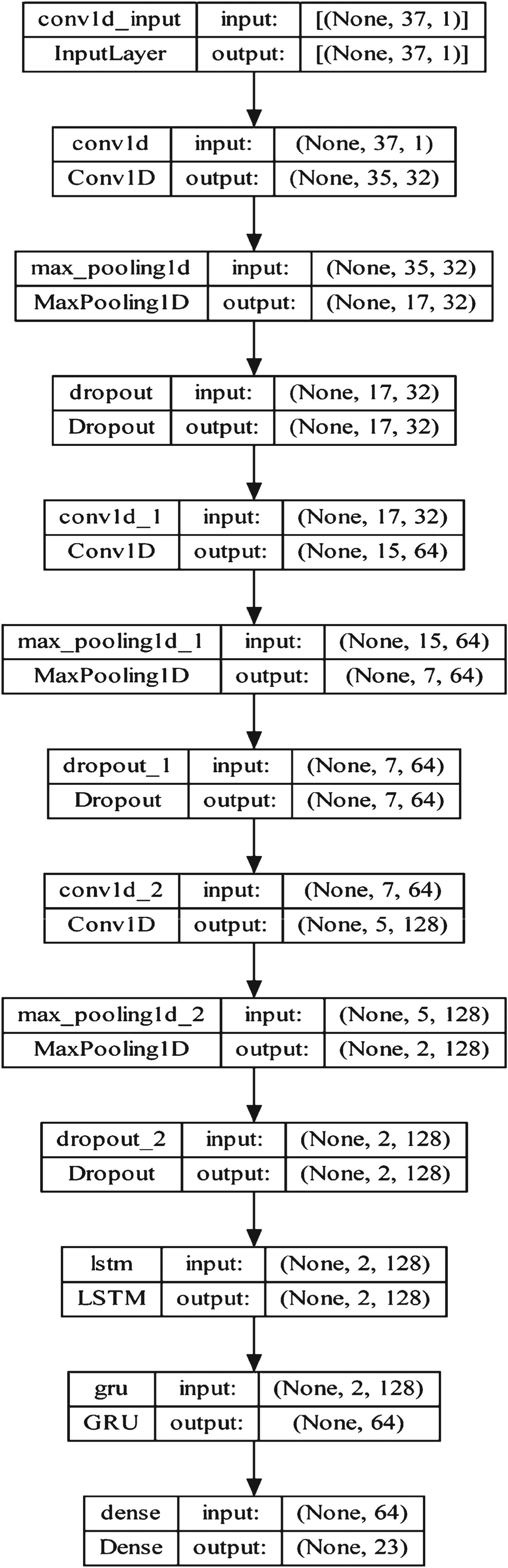
Optimized deep ensemble classifier.
Further, the PCF optimization that tunes the parameters of the ensemble model is described in the below section.
The PCF optimization is developed by integrating hunting as well as feeding characteristics (PBO) [9], (COA) [3], (CSO) [1], and (GWO) [12] of several families like Felis, Ursis, and Canis, which tracks the method of predating. In this case of PCF optimization, the hunting features as well as the feeding phenomenon are included in the proposed optimization. The advantages of PCF optimization emphasize the optimal convergence rate than other typical optimizations. The different phases involved in the developed optimization are explained as follows
Population Initialization:
In the initial phase, the entire number population such as 
The value of fitness feature is assumed while adapting the canis with its surroundings, and agents within the region of seeking at the Canis process are expressed as,

Where,
Setting the Velocity:
The reference velocity for the population is fixed at the initial stage. When the value of fitness is less than the maximum time, then it continues the process of velocity equalization, otherwise, it automatically ends the entire process.

Equalization of Velocity:
The Ursis in (PBO) [9] simulates the hunting capacity in severe arctic territories, which comprises several distinctive search phases in spaces such as local and global search. In local searches, ursis catches the prey by encircling them, whereas in the global search, it is done through gliding ice floats as well as dynamic population. When the velocity of the entire system is equal to the maximum value, then the Ursis diverge from their normal position and attacks its prey through the following expression as,

When the velocity of the entire system is not equal to the maximum value, then the velocity is based on two conditions such as whether the velocity is less or not.
Moderate Velocity:
Canis is considered as an algorithm depending on population [3], which mimics other canis as well as follows in the adaptation to the communal features as well as the surroundings. Canis is the combination of both the evolutionary heuristic as well as swarm intelligence and delivers the equilibrium between discovery and its growth. In this algorithm, the population is subdivided into several groups, the Canis solution is referred to as the candidate, as well as the fitness costs, are referred to as the communal characteristics. When the velocity is not less, then it is referred to as moderate velocity, which is assumed by considering the candidates of Canis as,

When the velocity is less, then it is passed to the condition of Seeking Mode Pool (SMP), which is assumed by considering the candidates of Canis as,
Seeking Mode Pool(SMP): SMP includes two conditions such as equal to one and not equal to one, which are described below,
When the SMP is assumed as one, then it passes the condition of When the SMP is not equal to one, then the candidate included in the Felis of (CSO) [1] is assumed by the below expression,
Search Space Decision: When the condition is Termination: The condition of the velocity is moderate and the phase of both the exploration as well as exploitation is passed to the initial condition after terminating the entire process, which is referred to as a loop process while attaining the global optimal results. The flowchart of the entire process is described in Figure 6.


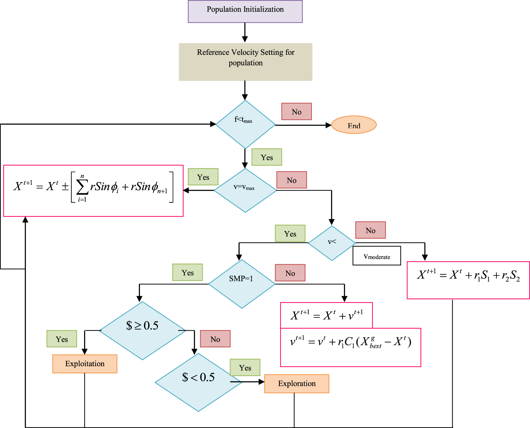
Flowchart of the entire process.
The PCF-deep ensemble model is utilized for classifying the imbalanced data, and the consequences of this system are presented here.
Experimental setup
Imbalanced data are classified with a PCF-based Deep Ensemble model through a Python tool executing on Windows 10 with 8 GB RAM. Thus, the implementation is carried out using three disease prediction datasets [10,19], and [11] for both testing and training the developed classifier.
Heart failure prediction dataset [10]
Cardiovascular diseases (CVDs) are considered the cause of death worldwide, which assumes nearly four CVDs out of 5 deaths are owing to heart attacks as well as strokes, and one-third of these deaths arise too early in people under the age of 70. Nowadays, heart failure is referred to as a common occurrence caused by CVDs and this database includes 11 features, which are utilized to calculate probable heart disease.
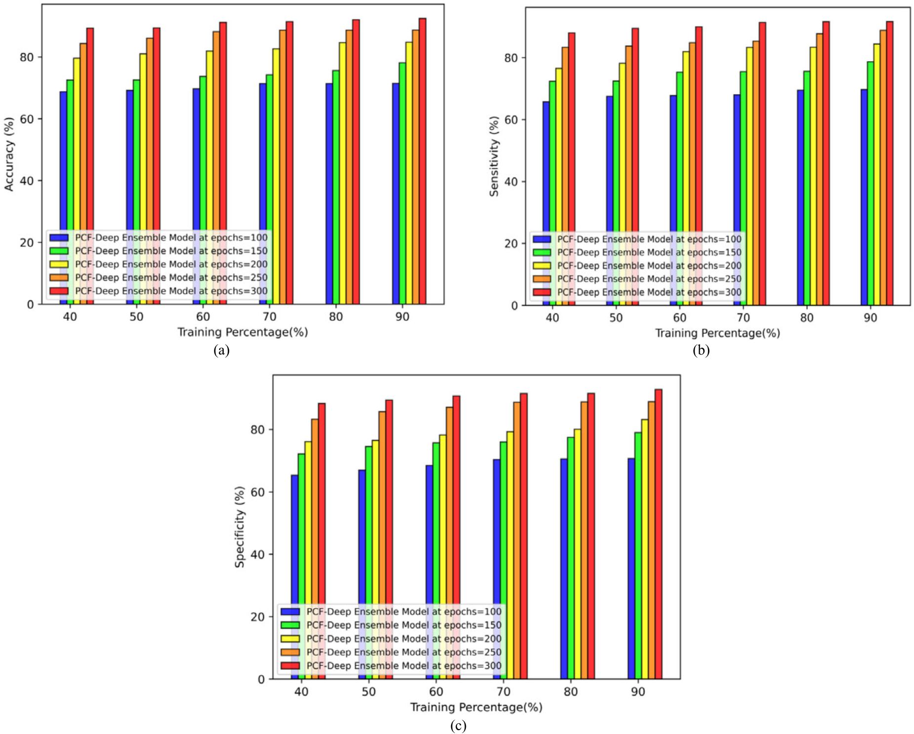
Performance evaluation with heart failure prediction dataset (a) accuracy, (b) sensitivity, and (c) specificity.
Stroke is considered the second cause of death worldwide, which is responsible for about 11% of entire deaths that are utilized to forecast whether a patient is probable to attain stroke depending on the input parameters like the status of smoking, age, gender, as well as several diseases. Each row present in the data delivers the relevant information regarding the concerned patient.
Hepatitis-C prediction dataset (Hepatitis-C prediction dataset) [11]
The dataset comprises the laboratory values of blood contributors and the patients of Hepatitis C as well as demographic values like age.
Comparative techniques
The merits of the PCF Optimization-based Deep Ensemble Algorithm are compared with the preceding techniques such as MLP, ANN, CNN-LSTM-GRU (CLG model), CNN-LSTM-GRU with Cheetah Optimizer(ChCLG), CNN-LSTM-GRU with Grey Wolf Optimizer(GCLG), CNN-LSTM-GRU with Coyote Optimizer(C2CLG), and CNN-LSTM-GRU with Cat Optimizer (CSCLG) is verified by enhancing the TP of the system’s comparative analysis.
Analysis with heart failure prediction dataset
Performance evaluation
The analysis of the imbalanced data classification in a database Heart Failure Prediction Dataset is depicted below, in which the performance evaluation is allowed to identify the classifier’s accuracy by changing epochs like 100, 150, 200, 250, and 300 relying on the training percentage (TP) of 90 is 77.87%, 83.48%, 85.95%, 89.71%, and 96.82% that is depicted in Figure 7 (a). The attained sensitivity values are 79.84%, 83.47%, 87.93%, 92.69%, and 95.58% by varying epochs such as 100, 150, 200, 250, and 300 respectively depending on the TP of 90 as illustrated in Figure 7 (b). The specificity values attained are 79.50%, 81.95%, 87.96%,90.62%, and 96.68% with variable epochs like 100, 150, 200, 250, and 300 concerning 90% of training as shown in Figure 7 (c).

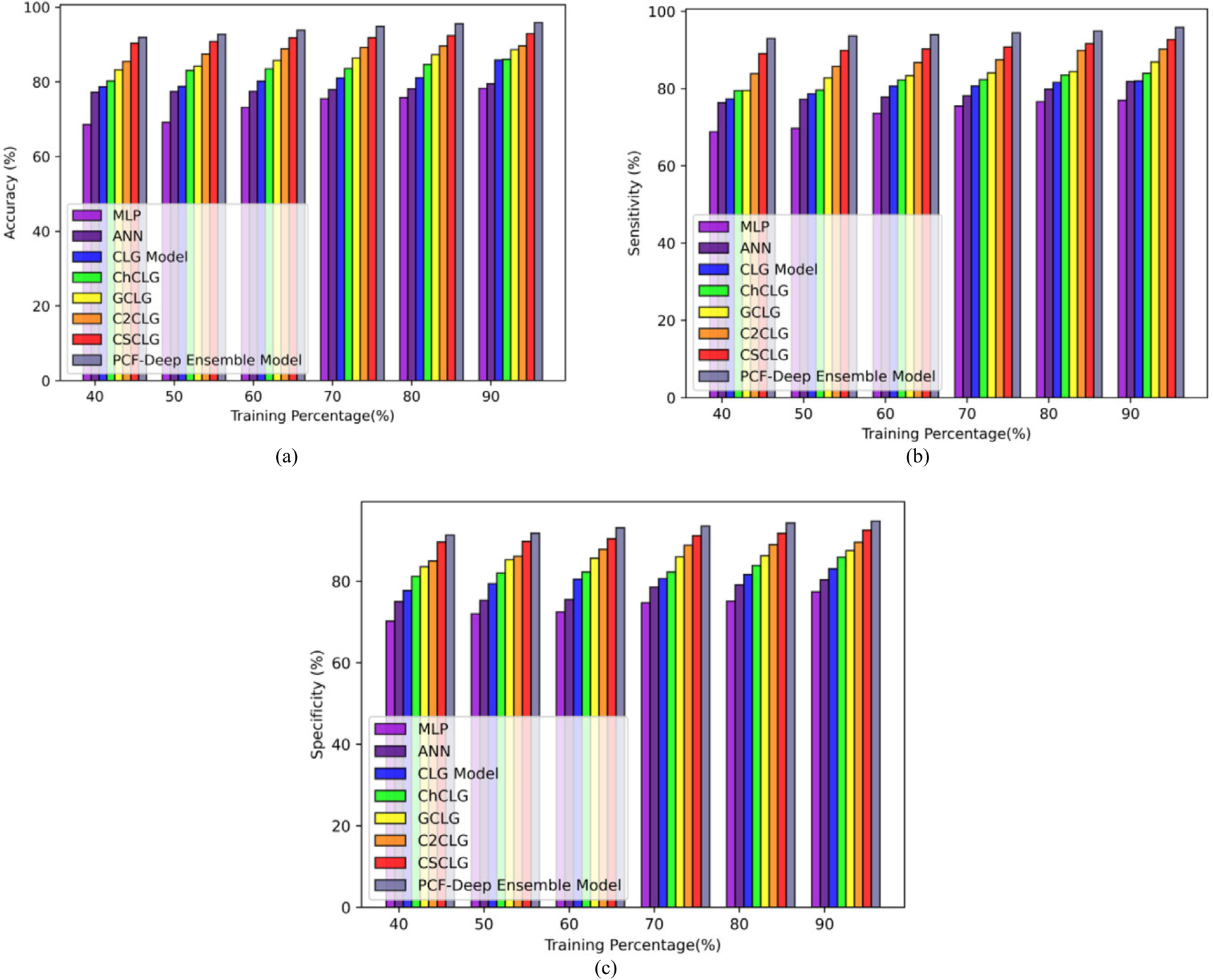
Comparative evaluation with heart failure prediction dataset (a) accuracy, (b) sensitivity, and (c) specificity.
The comparative evaluation depends on TP of 40, 50, 60, 70, 80, and 90 in the Heart Failure Prediction Dataset, and the evaluation describes that the established PCF-based deep ensemble model offered better values than other previous methods.The accuracy of the PCF-based deep ensemble model is 96.35% which is better than the prior techniques like MLP, ANN, CLG MODEL, CHCLG, GCLG, C2CLG, and CSCLG is 0.19%, 0.16%, 0.12%, 0.10%, 0.07%, 0.05%, and 0.04%. The sensitivity of the PCF-based deep ensemble model is 94.54%which is better than the prior methods such as MLP, ANN, CLG model, CHCLG, GCLG, C2CLG, and CSCLG is 0.18%, 0.13%, 0.09%, 0.08%, 0.07%, 0.04%, and 0.03%. Finally, the specificity of the developed model is 96.11% which is better than the prior methods such as MLP, ANN, CLG model, CHCLG, GCLG, C2CLG, and CSCLG is 0.19%, 0.17%, 0.12%, 0.09%, 0.07%, 0.06%, and 0.03%, which is indicated in below Figure 8 (a), (b), and (c).

Performance evaluation with stroke prediction dataset (a) accuracy, (b) sensitivity, and (c) specificity.
Performance evaluation
The performance evaluation of the imbalanced data classification in a database like the Stroke Prediction dataset is explained below, in which this analysis is allowed to detect the accuracy values of 80.21%, 84.50%, 90.27%, 93.71%, and 95.86% by varying epochs relying on the TP of 90 which is shown in Figure 9 (a). The values of sensitivity acquired as 78.70%, 82.42%, 90.68%, 93.72%, and 95.70% at epochs such as 100, 150, 200, 250, and 300 respectively depending on the TP of 90, which is depicted in Figure 9 (b). Finally, the specificity value is obtained with variable epochs like 100, 150, 200, 250, and 300 concerning the 90% of training is 79.59%, 83.48%, 90.07%, 92.82%, and 94.51% as shown in Figure 9 (c).
Comparative evaluation
The comparative evaluation relying on TP of 40, 50, 60, 70, 80, and 90 in the Stroke Prediction dataset, the examination describes that the PCF-based deep ensemble model offered better values than other prior methods. The accuracy of the PCF-based deep ensemble model is 95.91%which is better than the prior approaches such as MLP, ANN, CLG model, ChCLG, GCLG, C2CLG, and CSCLG is 0.18%, 0.17%, 0.10%, 0.10%, 0.08%, 0.07%, and 0.03%. The sensitivity of the PCF-based deep ensemble model is 95.87%, which is better than the prior techniques such as MLP, ANN, CLG model, ChCLG, GCLG, C2CLG, and CSCLG is 0.20%, 0.15%, 0.15%, 0.12%, 0.09%, 0.06%, and 0.03%. Finally, the specificity is 94.79% for the established model which is better than the prior methods such as MLP, ANN, CLG model, ChCLG, GCLG, C2CLG, and CSCLG is 0.18%, 0.18%, 0.12%, 0.09%, 0.08%, 0.06%, and 0.02%, which is revealed in below Figure 10 (a), (b), and (c).
Comparative evaluation with stroke prediction dataset (a) accuracy, (b) sensitivity, and (c) specificity.
Performance evaluation
The performance evaluation of the imbalanced data classification in a database like the Hepatitis-C prediction dataset is described below. The accuracy values obtained are 71.45%, 78.12%, 84.79%, 88.73%, and 92.53% by altering the epochs like 100, 150, 200, 250, and 300 respectively relying on the TP of 90 which is shown in Figure 11 (a). The sensitivity values are acquired by varying the epochs such as 100, 150, 200, 250, and 300 depending on the TP of 90 is 69.68%, 78.70%, 84.44%, 88.83%, and 91.68% as shown in Figure 11 (b). The specificity value is obtained by varying the epochs like 100, 150, 200, 250, and 300 concerning the 90% of training is 70.70%, 78.98%, 83.20%, 88.90%, and 92.83%as shown in Figure 11 (c).
Performance evaluation with Hepatitis-C prediction dataset (a) accuracy, (b) sensitivity, and (c) specificity.
The comparative evaluation depends on the TP of 40, 50, 60, 70, 80, and 90 in the Hepatitis-C prediction dataset, the analysis describes that PCF based deep ensemble model offered better values than other prior methods. The accuracy of the PCF-based deep ensemble model is 92.79, which is better than the prior approaches such as MLP, ANN, CLG model, ChCLG, GCLG, C2CLG, and CSCLG with the values of 0.30%, 0.28%, 0.14%, 0.13%, 0.09%, 0.05%, and 0.03% respectively. The sensitivity of the PCF-based deep ensemble model is 92.90 which is better than the prior techniques such as MLP, ANN, CLG model, ChCLG, GCLG, C2CLG, and CSCLG by 0.29%, 0.25%, 0.16%, 0.12%, 0.07%, 0.06%, and 0.04% respectively. Finally, the specificity of the PCF-based deep ensemble model is 92.63 which is better than the prior models such as MLP, ANN, CLG model, ChCLG, GCLG, C2CLG, and CSCLG with the improvement of 0.31%, 0.26%, 0.16%, 0.13%, 0.07%, 0.07%, and 0.03%that is depicted in below Figure 12 (a), (b), and (c).
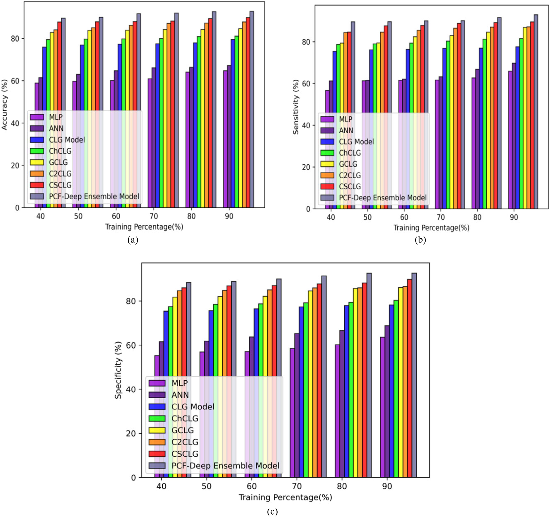
Comparative evaluation with Hepatitis-C prediction dataset (a) accuracy, (b) sensitivity, and (c) specificity.
This section portrays the comparative discussion of the developed approach, which is utilized for classifying the imbalanced data with the previous approaches. Thus, it represents that the proposed model is enhanced and achieves better results when compared with the existing techniques that are shown in Table 2. The PCF-deep ensemble model consistently demonstrates higher accuracy across all TPs (Heart Failure Prediction Dataset, Stroke Prediction dataset, Hepatitis-C prediction dataset) compared to existing methods. This improvement in accuracy can be attributed to several factors, such as feature engineering, algorithm selection, or model architecture. It is essential to highlight the specific features or methodologies employed in the proposed method that contribute to this accuracy boost. Sensitivity measures the ability of the model to correctly identify positive instances (e.g., correctly identifying minority class samples in imbalanced data). The PCF-based deep ensemble model consistently shows improved sensitivity. This suggests that it is better at identifying true positive cases, which is crucial in applications like medical diagnoses, fraud detection, and more. The enhancements in sensitivity are due to better data preprocessing, feature selection, or a more advanced classification algorithm. The PCF-based deep ensemble model also excels in specificity, indicating fewer false positives, which is vital in reducing false alarms.
Comparative discussion.
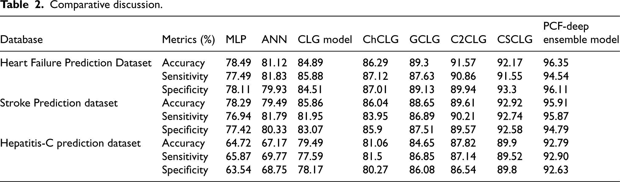
Comparative discussion.
Figure 13 depicts the computational analysis conducted for the proposed model and the existing techniques, in which techniques such as MLP, ANN, CLG model, ChCLG, GCLG, C2CLG, and CSCLG attained computational times of 0.044 ms, 0.037 ms, 0.030 ms, 0.024 ms, 0.037 ms, 0.029 ms, and 0.021 ms while the established model attained the computational time of 0.008 ms for iteration 20 which is minimized compared with other previous techniques. At iteration 100, the techniques including the MLP, ANN, CLG model, ChCLG, GCLG, C2CLG, and CSCLG reached the computational times of 0.043 ms, 0.036 ms, 0.030 ms, 0.023 ms, 0.036 ms, 0.029 ms, and 0.020 ms, in which the established model attained 0.007 ms which is low compared with other conventional approaches and revealed the efficiency of the PCF based deep ensemble model.
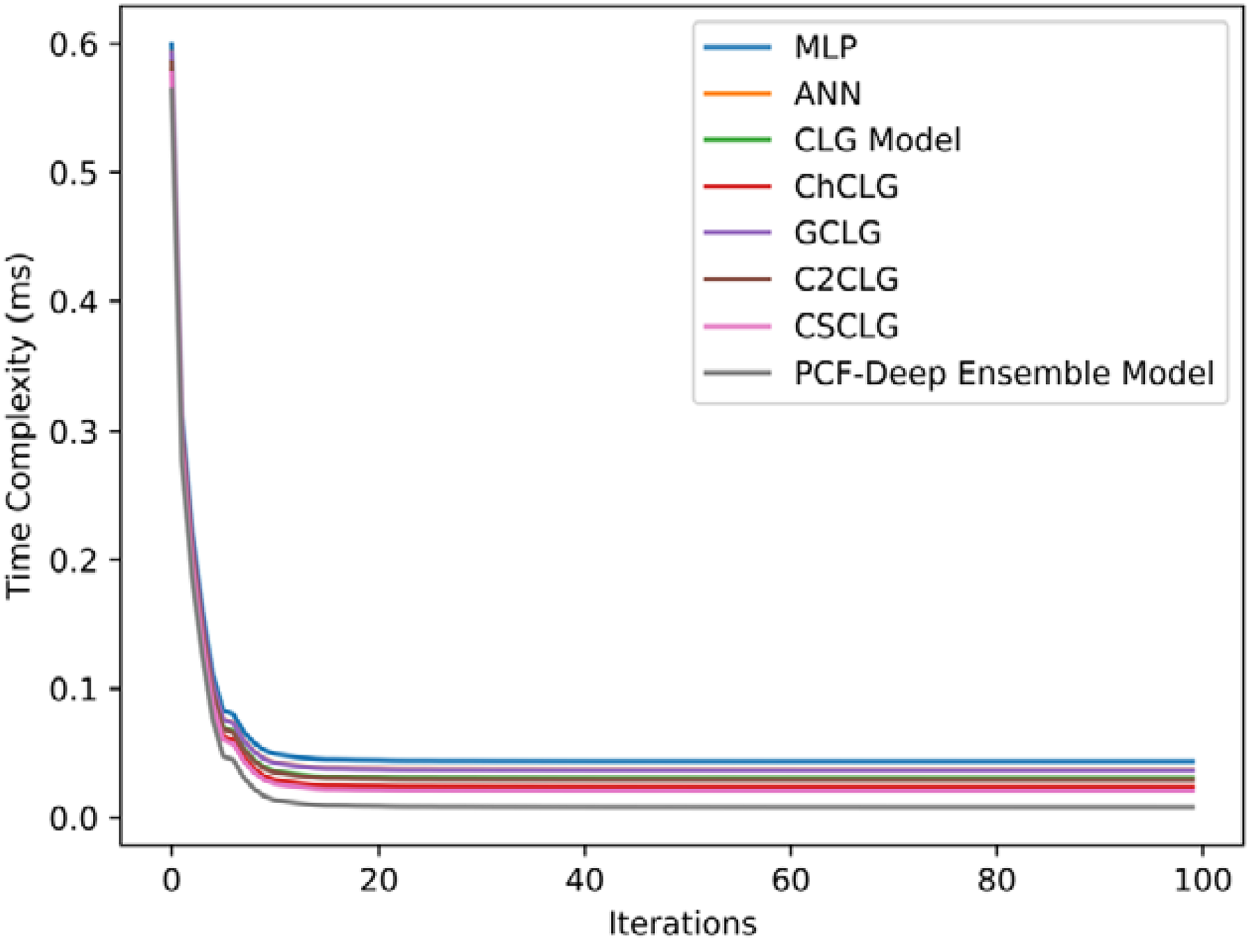
Computational analysis.
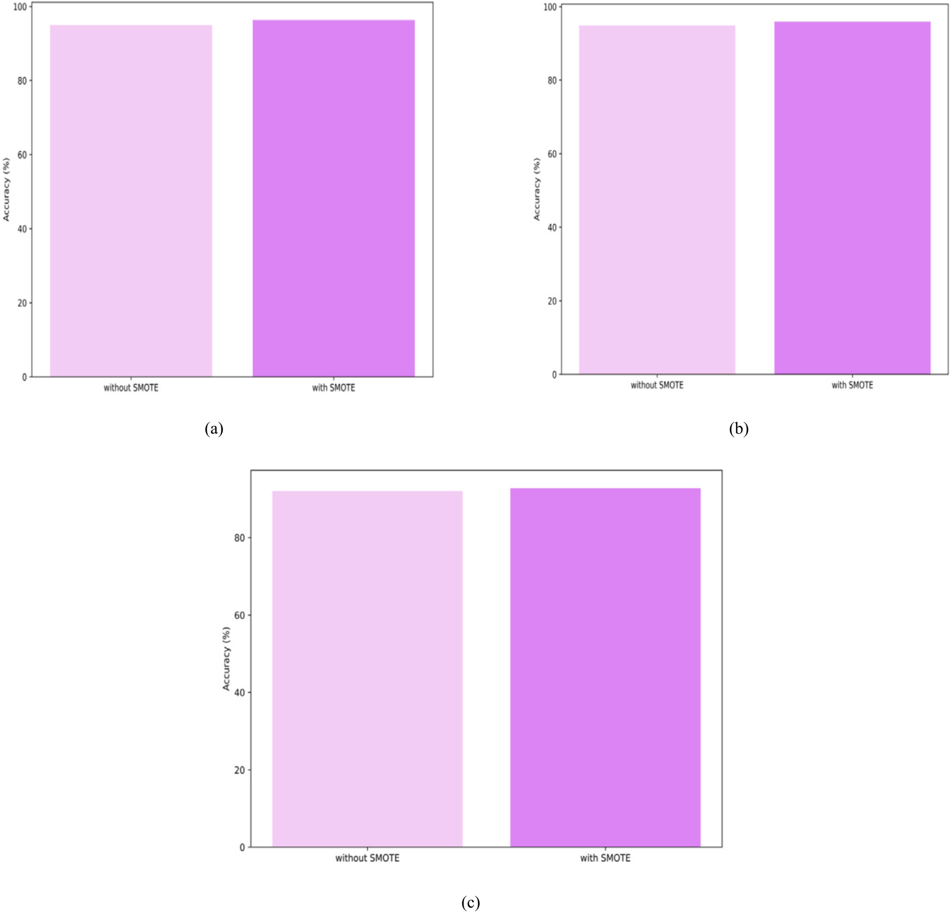
Ablation study, (a) heart failure prediction dataset, (b) stroke prediction dataset, and (c) Hepatitis-C prediction dataset.
The ablation study is conducted for the developed Imbalanced data classification approach, in which the performance of the PCF-deep ensemble model is examined with the process of the SMOTE data balancing and without the SMOTE. Figure 14 depicts the ablation study conducted for the established approach concerning the datasets Heart Failure Prediction Dataset, Stroke Prediction dataset, and Hepatitis-C prediction dataset. Figure 14 a) depicts that the PCF-based Deep Ensemble model attained an accuracy of 94.97% without SMOTE and 96.35% with SMOTE concerning the Heart Failure Prediction Dataset. Further, the PCF-based Deep Ensemble model attained an accuracy of 94.89% without SMOTE and 95.91% with SMOTE utilizing the Stroke Prediction dataset. Finally, the developed model attained accuracy values of 92.02% and 92.79% for without and with the SMOTE approach respectively utilizing the Hepatitis-C prediction dataset. From the ablation study, it is clear that the SMOTE approach has more impact on the accuracy of the PCF-deep Ensemble model.
Conclusion
The present research develops the PCF-deep ensemble model for Imbalanced data classification, which includes the framework of SMOTE for data balancing. The ED-based GE has been utilized in feature extraction for extracting the features. These extracted features are passed to the PCF Optimization for handling the incremental data, in which the developed PCF optimization integrates the characteristics of hunting as well as feeding behavior of the animals such as Felis, Canis, as well as Ursis for tuning the classifier to attain the best performance as well as to classify the model for handling the imbalanced big data. Thus, the accuracy, sensitivity, as well as specificity of the Heart Failure Prediction Dataset attained values of 96.35%, 94.54%, and 96.11%, whereas the Stroke Prediction dataset acquired values of 95.91%, 95.87%, and 94.79% for the accuracy, sensitivity, and specificity respectively, and finally, Hepatitis-C prediction dataset obtained the values of 92.79%, 92.90%, and 92.63% for the corresponding metrics at the TP of 90. In the future, the current research will be expanded to include alternative classifiers and algorithms, to achieve enhanced performance for IDC while ensuring greater scalability. This extension will enable the research to explore a broader range of techniques and strategies to address IDC challenges and adapt to diverse applications.