Predicting fringe visibility in dual-phase grating interferometry with polychromatic X-ray sources

Abstract

Dual phase grating X-ray interferometry is radiation dose-efficient as compared to common Talbot-Lau grating interferometry. The authors developed a general quantitative theory to predict the fringe visibility in dual-phase grating X-ray interferometry with polychromatic X-ray sources. The derived formulas are applicable to setups with phase gratings of any phase modulation and with either monochromatic or polychromatic X-rays. Numerical simulations are presented to validate the derived formulas. The theory provides useful tools for design optimization of dual-phase grating X-ray interferometers.

Keywords

X-ray imaging X-ray interferometry

1 Introduction

Currently, the Talbot–Lau X-ray interferometry is widely used for X-ray differential phase contrast imaging [1 –20]. In the Talbot–Lau grating-based interferometry, a phase grating is employed as a beam splitter to split the X-ray into diffraction orders. The interference between the diffracted orders forms intensity fringes. The sample imprints the X-ray beam with the phase shifts, and distorts the intensity fringes. By analyzing the fringes, a sample attenuation, phase gradient, and dark field images [1 –10] are reconstructed. To increase the grating interferometer’s sensitivity, fine-pitch phase gratings of periods as small as a few micrometers should be used. Nevertheless, in medical imaging and material science applications, it is only feasible to utilize common imaging detectors whose pixels are of a few tens of micrometers. To enable fringe detection with common image detectors, one method is to use a fine absorbing grating to indirectly detect fringe patterns through grating scanning. This is also known as the phase stepping procedure [1 –4]. However, the absorbing grating blocks more than half of the sample-exiting X-ray, and it will increase the radiation dose for a given imaging exam. In addition, the phase stepping procedure itself is cumbersome, especially for tomography in which phase stepping is required for each angular view. Another method is to use the brute-force geometric magnification to resolve the fine intensity fringe generated by a fine-pitch phase grating. In such an inverse geometry, the setup of the phase grating is placed close to the source such that the fringe period is geometrically magnified by a factor of a few tens or more [14–16 , 21]. A disadvantage of this kind of setup is that it stipulates a large system length because of the high-magnification factor [14, 21].

Recently, the advantages of dual-phase grating X-ray interferometry were demonstrated through the pioneering studies of [22, 23]. Different from Talbot-Lau interferometry, this new interferometry technique adds one more phase grating and ditch away the absorbing grating, which is the culprit for radiation dose inefficiency of Talbot-Lau interferometry. One of its unique advantages is that it enables the use of a common image detector to directly resolve the intensity fringes generated by the fine-pitch gratings without the need of absorbing grating and keeps the system length in check. A typical dual-phase grating interferometer employs two phase gratings, G₁ and G₂, as the beam splitters, shown in Fig. 1. The multiple splitted waves overlap and interfere with one another, creating the intensity fringes of different diffraction orders. The imaging detector, through its pixel averaging effects, only resolves the beat patterns of the large periodicities. This indicates that a common imaging detector with a resolution of tens of micrometers is able to resolve the fringes generated by the fine phase gratings with a pitch of few micrometers. Therefore unlike the Talbot–Lau setups, the dual-phase grating enables direct fringe detection without the need of the absorbing grating. Moreover, in contrast to the inverse geometry setups, the dual-phase grating keeps the system’s length compact because the fringe period can be conveniently tuned by adjusting the grating spacing without an increase in the size of the system. In designing an interferometer, it is desirable to be able to quantitatively predict the fringe visibility, which is the figure of merit for interferometer performance. A high fringe visibility reduces the quantum noise in differential phase images and increases the interferometry sensitivity. To predict the fringe visibility, one needs to develop a quantitative theory of dual-phase grating interferometry. Considering the efforts of seeking a theoretical understanding of the dual-phase grating interferometry, [22] derived an implicit expression of the fringe visibility for the 1^st diffraction order, which is applicable only to monochromatic X-ray source and the π/2-grating setup. Moreover, the fringe visibility values have to be extracted through a numerical computation from this implicit expression. It will be more convenient for a system design optimization if one can derive explicit expressions of the fringe visibility. In addition, in [22], the detector-pixel binning effects are not considered. However, the pixel averaging effects play an important role in the fringe detection. Therefore, a complete quantitative theory is required for establishing a rigorous analysis, and shedding a new light on the design optimization of this new technique. Recently we developed a quantitative theory of a dual-phase grating interferometry, using the Wigner distribution formalism [24]. As is demonstrated in this previous study [24], we derived and validated these explicit expressions of the fringe visibility for any dual grating setup. These expressions are in terms of elementary functions of the grating phase modulation (π/2- or π-shifting or other values), the interferometer geometry such as the grating pitch as well as the spacing between the two gratings and the X-ray wavelength, the focal spot width, and the detector’s pixel size. These formulas of the fringe visibility provide a useful tool for system optimization. Quite recently, a study obtained the same results as ours [24] for the π-grating setups by using the theory of dynamic wave analysis [25].

Fig. 1

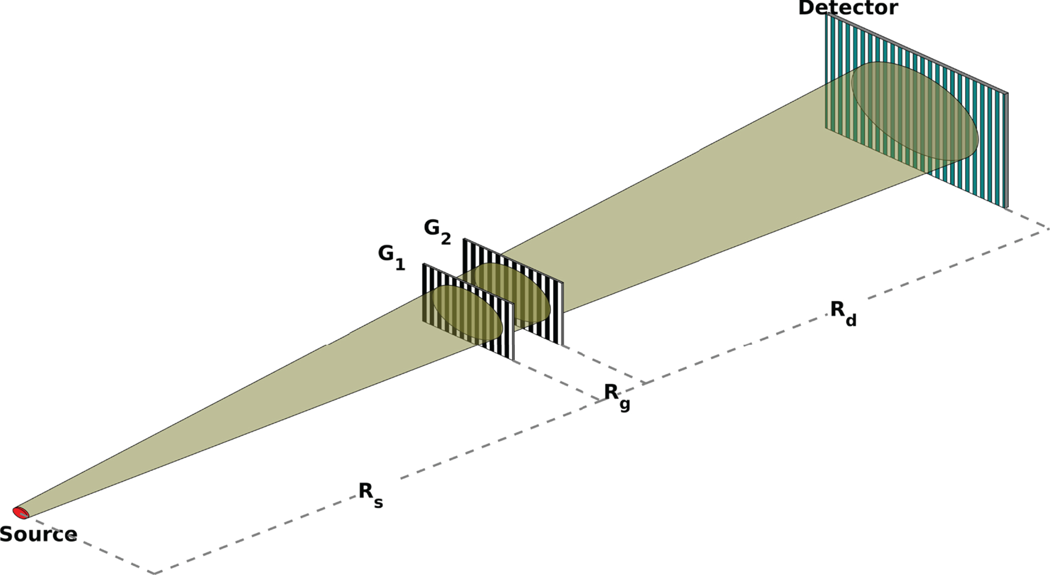
Schematic of an X-ray dual-phase grating interferometer.

In these published theoretical analysis of the dual phase grating interferometry [22 , 25], all assumed the use of monochromatic X-ray source, while most imaging applications employ polychromatic sources such as X-ray tubes, which emit X-ray of broad spectrum. Then how can one predict fringe visibility of the setups with polychromatic X-ray? At the first glance, one might think that an X-ray spectral integral of the visibility formula derived in [24] would predict fringe visibility with polychromatic X-ray. Unfortunately, this is not true.

To clarify this issue, note that the fringe visibility, V, of a fringe pattern is defined as V = (I_max - I_min)/(I_max + I_min), where I_max and I_min are the maximum and minimum intensities, respectively. We may denote the contribution of the n-th fringe-harmonics to the fringe visibility by V_n. The fringe visibility receives the contributions from all harmonics of the intensity fringe pattern, though the contributions from V_n of n ≥ 3 are negligible in most of practical cases [24]. Mathematically, the intensity fringe visibility V is not a weighted sum of V₁ and V₂, rather it is indeed a complicate function of V₁ and V₂, as is shown below. The fringe visibility formulas derived in [24] are applicable only for π/2- or π-gratings with a monochromatic X-ray setup at the grating design energies. In that work we showed that, in π/2-dual grating setups, V₁ dominates the contribution to fringe visibility [24]. On the other hand, for π-dual grating setups, we found that V₁ is diminishing and V₂ dominates for fringe visibility [24].

For the setups with polychromatic X-ray, the phase-shift value of a grating varies with photon energies. For example, a π-grating of design energy 15-keV X-ray becomes π/2-grating for 30-keV X-ray, assuming absence of absorption edges in the spectrum’s energy range. Hence a grating will exhibit various phase shifts for a broad-band X-ray spectrum. Consequently, both V₁ and V₂ would contribute to fringe visibility in setups with polychromatic X-ray. Moreover, as will be shown below, the intensity fringe visibility V is indeed a nonlinear function of V₁ and V₂.

In order to provide a design optimization tool for dual phase grating interferometry, in this work we set out to derive formulas to predict the intensity fringe visibility V of dual phase grating setups with polychromatic X-ray. The formulas are validated by numerical simulations. In Section 2, we briefly explain the formation of the intensity fringe patterns derived in [24]. Other than the formulas in [24] where the two phase gratings are assumed to be identical, a more general resolvable intensity fringe pattern representation is presented for different phase gratings. In Section 3.1, we derive the formulas of the fringe visibility as a function of the X-ray photon energy. These formulas present a useful tool for optimizing the fringe visibility in polychromatic setups. In Section 3.2, we present numerical simulations to verify the formulas derived in Section 3.1. We summarize and conclude this study in Section 4.

2 Methods

We consider a typical setup of a dual-phase X-ray interferometry as shown in Fig. 1, in which two phase gratings, G₁ and G₂, with a duty cycle of 0.5 are employed. Let R_s be the source-to-G₁ distance, R_d be G₂-to-detector distance, and R_g be the spacing between the two phase gratings (Fig. 1). In discussion, we define the geometric magnification factors from G₁ and G₂ to detector plane as M_{g
₁} and M_{g
₂}, respectively, as demonstrated in the equation below: $M_{g_{1}} = \frac{R_{s} + R_{g} + R_{d}}{R_{s}}; M_{g_{2}} = \frac{R_{s} + R_{g} + R_{d}}{R_{s} + R_{g}} .$ (1) Notably, in the absence of the G₂-grating, a diffraction order of the intensity pattern generated by only the G₁ grating would be represented by exp [i2π (l · x)/(M_{g
₁} · p₁)], where l is an integer indexing the diffraction order, and p₁ is the period of the G₁. Similarly, in absence of the G₁-grating, a diffraction order of the intensity pattern generated by only the G₂ grating would be represented by exp [i2π (r · x)/(M_{g
₂}p₂)], where r indexes the diffraction order of the fringe in the absence of the G₁-grating with a p₂ period of G₂. The X-ray irradiance involves a cross-modulation between the fringe patterns generated by the phase gratings G₁ and G₂ of different diffraction orders (l, r): exp [i2πx · (l/(M_{g
₁}p₁) + r/(M_{g
₂}p₂))]. As a result, the X-ray irradiance at the detector entrance is a weighted sum of different diffraction orders (l, r) [24]: $I (x, y) = \frac{I_{in}}{M_{{g_{1}}^{2}}} \cdot \sum_{l, n, r, s \in ℤ} μ (- \frac{λ R_{d}}{M_{1}} \cdot [\frac{l}{M_{g_{1}} p_{1}} + \frac{r}{M_{g_{2}} p_{2}}] - l \frac{λ R_{g}}{M_{1} p_{1}}) \times \times a_{l + n} a_{n}^{*} b_{r + s} b_{s}^{*} \times exp [- i 2 π (\frac{l (l + 2 n) λ R_{g}}{2 M_{1} p_{1}^{2}})] \times \times exp [- i 2 π (\frac{(l + 2 n) λ R_{d}}{2 M_{1} p_{1}}) \cdot (\frac{l}{M_{g_{1}} p_{1}} + \frac{r}{M_{g_{2}} p_{2}})] \times \times exp [- i 2 π (\frac{(r + 2 s) λ R_{d}}{2 p_{2}}) \cdot (\frac{l}{M_{g_{1}} p_{1}} + \frac{r}{M_{g_{2}} p_{2}})] \times \times exp [i 2 π (\frac{l}{M_{g_{1}} p_{1}} + \frac{r}{M_{g_{2}} p_{2}}) x],$ (2) where M₁ = (R_s + R_g)/R_s, a_l, and b_r represent the Fourier coefficients of the G₁ and G₂ gratings, respectively: $\begin{matrix} G_{1} (x) = \sum_{l \in ℤ} a_{l} exp [i 2 π \frac{lx}{p_{1}}]; G_{2} (x) = \sum_{r \in ℤ} b_{r} exp [i 2 π \frac{rx}{p_{2}}] . \end{matrix}$ (3) The term μ (- λR_d/M₁ · (l/(M_{g
₁}p₁) + r/(M_{g
₂}p₂)) - lλR_g/(M₁p₁)) in Eq. (2) is the coherence degree associated with the diffracted order (l, r).

Notably, the intensity fringe of order (l, r) has a periodicity of p_fr = (l/(M_{g
₁}p₁) +1/(M_{g
₂}p₂)) ^-1. Because the grating periods are only a few micrometers, most of the interference fringes are too fine to be detected using a common imaging detector. However, among the fringe patterns, there are beat patterns formed by those diffraction orders characterized by l = - r when p₁ ≈ p₂. These beat patterns are generated by the interference beat patterns. The beat pattern consists of a fundamental frequency and its harmonics. The period of the 1^st harmonics of the beat patterns is [24] $p_{fr} = (\frac{- 1}{M_{g_{1}} p_{1}} + \frac{1}{M_{g_{2}} p_{2}})^{- 1} = \frac{R_{s} + R_{g} + R_{d}}{R_{g} / p_{2} + R_{s} (1 / p_{2} - 1 / p_{1})} .$ (4) However, the period of the l-th harmonics is p_fr/l. According to Eq. (4), the beat pattern periods can be much larger than the grating periods, p₁ and p₂, with the proper geometric setup, M_{g
₁} and M_{g
₂}. For example, if the system geometry is set in such a way that R_s + R_d ⪢ R_g and p₁ ≈ p₂, then p_fr ⪢ p₁, p₂. Consequently, the beat pattern may be resolved by a common imaging detector. Nevertheless, as long as detector period is p_D ⪢ p₁, p₂, the detector renders all other fine fringes to the constant background because of detector-pixel averaging effect. Note that this detector-pixel averaging will damp the beat pattern contrast as well. As we showed in [24], the pixel averaging accrues a factor, sinc (lp_D/p_fr), for order l, for order l, where sinc (x) ≡ sin(πx)/(πx). It should be noted that the effect of the pixel averaging on the fringe visibility was not taken into account in [22]. Similar to the derivation in [24], by extracting the diffracted orders of l = - r from Eq. (2), the resolvable intensity fringe pattern, I_res, can be obtained: $I_{res} (x, y) = \frac{I_{in}}{M_{g_{1}}^{2}} \cdot \sum_{l \in ℤ} μ (- l λ \frac{R_{s}}{p_{0}}) \cdot sinc (l \frac{p_{D}}{p_{fr}}) \times \times C_{l} (\frac{p_{1}}{p_{0}} R_{s}, λ, p_{1}, Δ ϕ_{1}) \cdot C_{- l} (\frac{p_{2}}{p_{fr}} R_{d}, λ, p_{2}, Δ ϕ_{2}) \times exp [- i 2 π l \cdot \frac{x}{p_{fr}}],$ (5) where $p_{0} = \frac{R_{s} + R_{g} + R_{d}}{R_{g} / p_{1} + R_{d} (1 / p_{1} - 1 / p_{2})},$ (6) is the source cycle [22, 26]. In Eq. (5), μ (- lλR_s/p₀) is the coherence degree associated with the diffracted order, l, sinc (lp_D/p_fr) is the detector-pixel averaging effect, and functions C_l (·) and C_-l (·) are related to the Fourier coefficients of the intensity fringe generated by a single phase grating interferometer [17]. These Fourier coefficients can be generally denoted by C_l (d, λ, p_g, Δϕ_g), where d is the effective diffraction distance, p_g is the grating pitch and Δϕ_g is the grating’s phase modulation. We have derived explicit expressions for C_l (d, λ, p_g, Δϕ_g) to facilitate the quantitative analysis of the grating interferometry [17]: $C_{l} (d, λ, p_{g}, Δ ϕ_{g}) = {\begin{matrix} 1, & if l = 0, \\ - 2 (1 - cos Δ ϕ_{g}) \times \\ \times (- 1)^{⌊ 2 l λ d / p_{g}^{2} ⌊} \cdot \frac{sin (l^{2} π λ d / p_{g}^{2})}{l π}, & if l = 2 k \neq 0, \\ - i 2 sin Δ ϕ_{g} \cdot \frac{sin (π λ d / p_{g}^{2} \cdot l^{2})}{π l}, & if l = 2 k + 1 . \end{matrix}$ (7) From Eq. (7) it can be observed that $C_{l} (d, λ, p_{g}, Δ ϕ_{g}) = C_{- l}^{*} (d, λ, p_{g}, Δ ϕ_{g})$ , where a^∗ represents the complex conjugate of a.

Equation (5) is the key equation for the analysis of beat pattern periods and fringe visibility. In following sections, we will comprehensively discuss how to properly setup the geometries for predicting a high fringe visibility based on Eq. (5).

3 Results

3.1 Fringe visibility as a function of X-ray photon energy

Fringe visibility is a common figure of merit for an interferometer’s performance [1 –4]. This is because the formation of a high-modulation fringe pattern is crucial to a robust interferometry. To examine the fringe visibility, we consider the detected intensity fringe without a sample. The fringe visibility, V, of a fringe pattern is defined as V = (I_max - I_min)/(I_max + I_min), where I_max and I_min are the maximum and minimum intensities, respectively. Equation (5) shows that the fringe visibility depends on the dual grating phase modulation, spatial coherence of the illumination, system geometry setup, and X-ray spectrum. In a previous study, we derived and validated the formulas of the fringe visibility, assuming a monochromatic X-ray of the grating design energy [24]. In that study, we demonstrated that the fringe visibility can be conveniently adjusted by tuning the G₁ - G₂ spacing [24]. However, in practice, most X-ray sources are polychromatic. The fringe visibility is X-ray energy dependent. The energy dependency of the fringe pattern is in two folds. First, the phase shift of a grating inversely scales with the photon energy. Second, the visibility coefficients, C_l, of the diffraction orders are energy-dependent as well. Therefore, to achieve design optimization, it is useful to derive an explicit formula to understand how the fringe visibility varies with the X-ray energy as well as the G₁ - G₂ spacing and predict the fringe visibility for the setups with polychromatic sources.

To achieve this, we combine Eqs. (7) and (5). For conciseness, we assume p₁ = p₂, Δϕ₁ = Δϕ₂ = (E_D/E) · Δϕ_d, and R_s = R_d. With this symmetric setup, we found that the detected intensity pattern in the absence of a sample is given by: $\begin{matrix} I_{res} (x, y; E) = \frac{I_{in}}{M_{g_{1}}^{2}} \cdot [1 + \sum_{l = 1}^{\infty} V_{l} (E, Δ ϕ_{d}) \cdot cos (2 π l \cdot \frac{x}{p_{fr}})], V_{l} (E, Δ ϕ_{d}) \equiv \frac{8}{π^{2} l^{2}} μ (- l λ \cdot \frac{R_{s}}{p_{0}}) \cdot sinc (l \cdot \frac{p_{D}}{p_{fr}}) \times \\ \times {sin}^{2} (π l^{2} λ \cdot \frac{R_{s}}{p \cdot p_{fr}}) \cdot g_{l} (E, Δ ϕ_{d}), g_{l} (E, Δ ϕ_{d}) = {\begin{matrix} {sin}^{2} (\frac{E_{D}}{E} Δ ϕ_{d}), & if l = 2 k + 1, \\ [1 - cos (\frac{E_{D}}{E} Δ ϕ_{d})]^{2}, & if l = 2 k, \end{matrix} \end{matrix}$ (8) where p_fr = p₀ = M₆p, M₆ = (R_s + R_g + R_d)/R_g.

We refer to V_l (E, Δϕ_d) in Eq. (8) as the visibility coefficient of the diffraction order, l. In Eq. (8), Δϕ_d is the gratings’ phase modulation at the design energy, E_D. To derive the fringe visibility formulas, the high diffraction orders made only a negligible contribution to the intensity fringe pattern. This is because factor $C_{l} (\frac{R_{s}}{M_{6}}, λ, p, Δ ϕ_{d}) \cdot C_{- l} (\frac{R_{d}}{M_{6}}, λ, p, Δ ϕ_{d})$ is proportional to l^-2 as demonstrated in Eq. (7). Consequently, the intensity modulation damps quickly with increasing diffraction orders. The degree of coherence, μ (- lλ · R_s/p₀), for an incoherent source such as a focal spot of an X-ray tube can be calculated using the Van Cittert-Zernike theorem. For example, for a focal spot of width of a, $μ (- l \frac{λ R_{s}}{p_{0}}) = sinc (l \cdot \frac{a}{p_{0}}) .$ (9) In addition, the degree of coherence and pixel-averaging factor, sinc (l · p_D/p_fr), both decrease with the increasing diffracted orders. Thus, to calculate the fringe visibility, it is enough to consider the first two diffraction orders in the intensity formula of Eq. (8). Therefore, in these practical cases, more often than not, the intensity fringe pattern can be expressed in a good approximation as follows: $I_{res} (x, y; E) = \frac{I_{in}}{M_{g_{1}}^{2}} [1 + V_{1} (E, Δ ϕ_{d}) \cdot cos (2 π \frac{x}{p_{fr}}) + + V_{2} (E, Δ ϕ_{d}) \cdot cos (4 π \frac{x}{p_{fr}})],$ (10) where the visibility coefficients, V₁ (E, Δϕ_d) and V₂ (E, Δϕ_d), are given by Eq. (8). In practice, the X-ray tubes are mostly used. Therefore, the measured intensity pattern I_res (x, y) is given by the spectral average of the intensity patterns at different photon energies. This indicates that: $\begin{matrix} I_{res} (x, y) = \frac{I_{in}}{M_{g_{1}}^{2}} [1 + V_{1} \cdot cos (2 π \frac{x}{p_{fr}}) + V_{2} \cdot cos (4 π \frac{x}{p_{fr}})], \\ V_{l} = \int V_{l} (E, Δ ϕ_{d}) \cdot S (E) d E, l = 1, 2, \end{matrix}$ (11) where S is the X-ray spectral distribution of the X-ray tube. The fringe visibility can then be found in Eq. (11):

$V = \frac{I_{\max} - I_{\min}}{I_{\max} + I_{\min}} = {\begin{matrix} \frac{V_{1} + 2 V_{2} + V_{1}^{2} / (8 V_{2})}{2 + V_{1} - V_{1}^{2} / (8 V_{2})}, & if V_{1} \leq 4 V_{2}, \\ \frac{V_{1}}{1 + V_{2}}, & if V_{1} > 4 V_{2} . \end{matrix}$ (12) Equation (11-formula) indicates that the intensity fringe visibility V is a nonlinear function of V₁ and V₂. It will play an important role in predicting the intensity fringe visibility of the setups with the polychromatic X-ray.

3.2 Numerical simulations

To validate the Eqs. (8–11-formula) for predicting the fringe visibility of the setups with the polychromatic X-ray, we compare the calculated fringe visibility using Eqs. (8–11-formula) to the one determined using the intensity patterns obtained from the numerical simulations of the wave propagation. Considering an interferometer with an X-ray tube, the setup consists of two identical π-shift phase gratings with a design energy of E_D = 20 keV. The system configuration is assumed as follows: the grating’s period, p = 1μm, and the source-G₁ distance, R_s, and the G₂-detector distance, R_d, are fixed to 450 mm. For the source, we assume that the tube is of a tungsten target and a rhodium filtration, and the tube operates at 34 kVp (a typical source setting employed in breast tomosynthesis). Figure 2 shows the X-ray spectrum of such a source. In addition, we assume that the focal spot has a width of 40μm, and the detector-pixel is 25μm in size. We calculated the visibility coefficients V₁ and V₂, using Eqs. (8–11) and the spectrum plotted in Fig. 2. Figure 3(a) shows how the calculated V₁ and V₂ vary with the gratings’ spacing R_g. The blue curve plots V₁ as a function of R_g while the red curve depicts how the V₂ varies with R_g. The visibility curve V = (max(I) - min(I))/(max(I) + min(I)) calculated using Eq. (11-formula) is shown in Fig. 3(b) as the solid blue curve.

Fig. 2

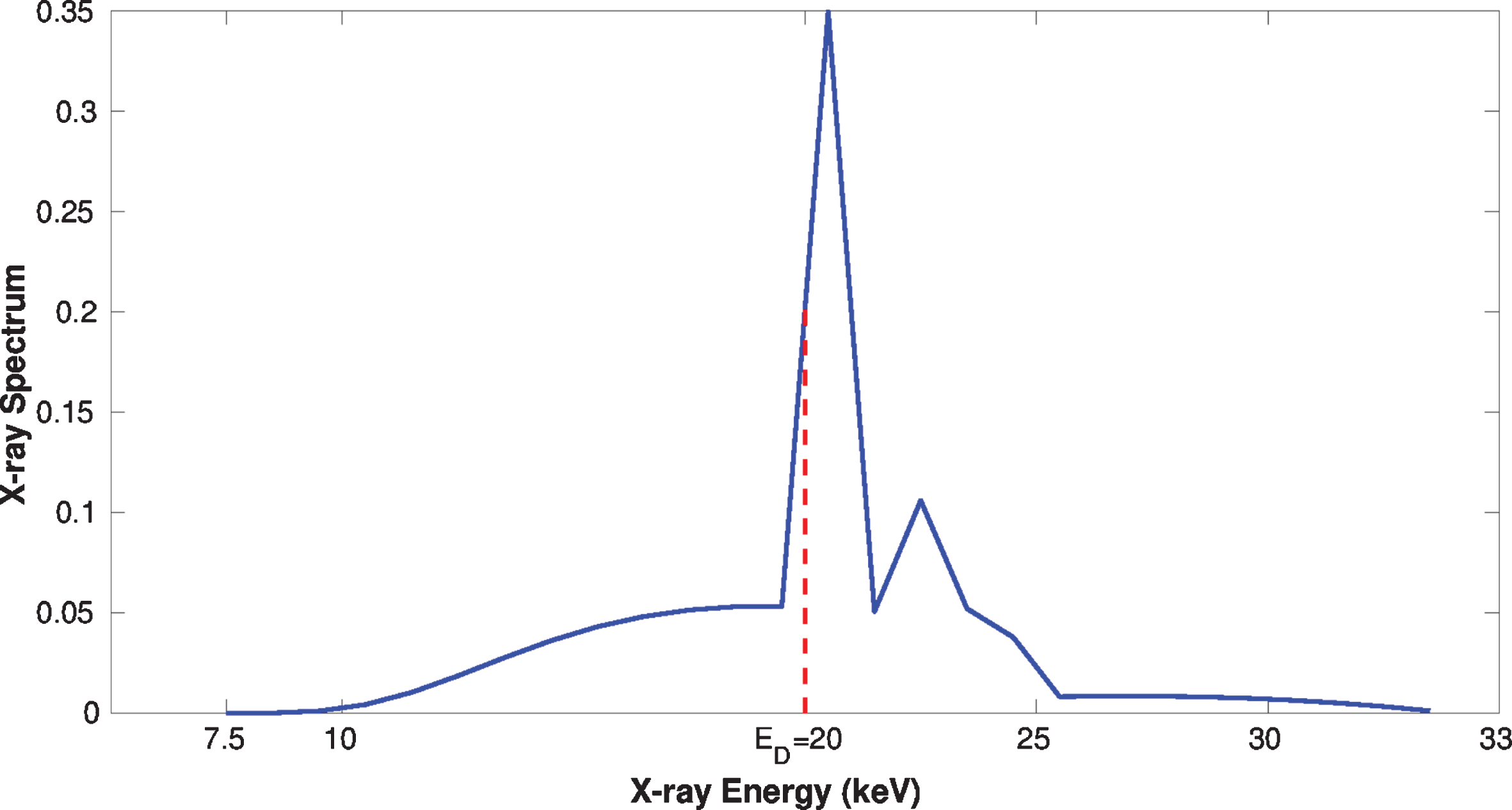
34 kV, Rh/Ag target/filter spectrum employed in the simulations.

Fig. 3

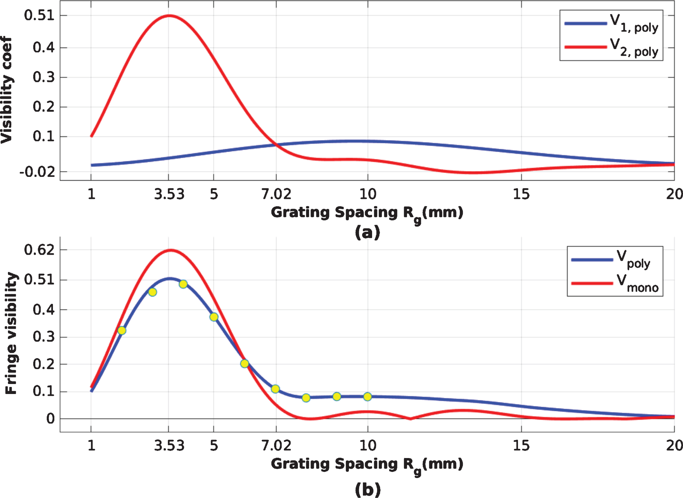
Plot of the fringe visibility with respect to the G₁-G₂ spacing R_g for two identical π phase gratings. In the figure, we assume that the dual-phase grating has a period, p = 1μm, and a phase shift, π, at the design energy, E_D = 20keV. A 34 kVp X-ray tube (Fig. 2) with focal spot of width a = 40μm is also assumed. The detector-pixel size is set to m. The geometry is set symmetrically with R_s = R_d = 450 mm and dual-grating spacing R_g changes from 1 mm to 20 mm. The blue and red curves shown in Fig. 3(a) represent the visibility coefficients, V₁ and V₂, respectively. The solid blue curve shown in Fig. 3(b) is the change of the theoretical visibility value, V = (max(I) - min(I))/(max(I) + min(I)), calculated from Eq. (11-formula) with respect to the G₁-G₂ spacing R_g. As a reference, the visibility curve of the monochromatic X-ray source is shown in Fig. 3(b) as the red curve. The yellow dots in Fig. 3(b) represent the measured fringe visibilities from the intensity patterns generated using the numerical wave propagation. For details, see text.

Figure 3(a) shows that V₂ ⪢ V₁ are the R_g values ranging from 1 mm to 6 mm. Therefore, in this range of R_g values, the fringe visibility is simply equal to the corresponding V₂ values in a good approximation. Because the R_g ranges from 8 mm to 15 mm, V₁ ⪢ V₂, the fringe visibility will simply be equal to the V₁ values. However, when R_g is between 6 mm and 8 mm, the values of V₁ and V₂ are comparable, and the visibility value will depend on both the V₁ and V₂.

To validate the fringe visibility of Eqs. (8–11-formula), we performed numerical simulations for the fringe patterns through wave Fresnel diffraction propagation. Recall the Fresnel wave propagation equation from R₁ to R₂ can be expressed as $E (ξ; R_{1} + R_{2}) = \frac{\sqrt{I_{in}}}{λ R_{2}} exp [- 2 π i \frac{R_{1} M}{λ}] \cdot exp [i π \frac{ξ^{2}}{λ R_{1} M}] \cdot (H ⊛ T) (ξ),$ (13) where I_in denotes the incident X-ray intensity at R₁, λ is the x-ray wave length, H (x) = exp [iπx² · M/(λR₂)], M = (R₁ + R₂)/R₁, and T (x) is the wavefront at the R₁ plane. The symbol ⊛ in above equation represents the convolution operator. The wavefront E can be numerically simulated through Fast Fourier Transform (FFT). Repeatedly applying the wave propagation from G₁ grating downstream to the G₂ plane and then (after multiplying the G₂ grating) downstream to the detector plane, one can numerically simulate the wavefront at the detector entrance. Once the wavefront is simulated, the intensity is acquired through I = |E²|. The fringe visibility is then measured through V = (max(I) - min(I))/(max(I) + min(I)). The measured fringe visibilities from the intensity patterns generated with numerical simulations are shown in yellow dots in Fig. 3(b), and the quantative values are listed in Table 1, for R_g = 2, 3, ⋯, 10 mm. The agreement between the blue curve and yellow dots validates the visibility formulas of Eq. (8-11-formula). Figure 3(a) shows that the V₂ peaks at approximately 50% for R_g values ranging from 3 mm to 4.5 mm. In this range of R_g values, according to Eq. (4), the fringe periods, p_fr/2, are in a range of 100 - 150 μm. Therefore, the fringes are well resolved by the detector because its pixels are of 25μm in size. Nevertheless, when the R_g ranges above 7 mm, both the V₁ and the V₂ diminish, and the fringe periods, p_fr/2, will be less than 65 μm. Apparently, this range of R_g values is not good for this interferometer. Comparing to the visibility curve of the monochromatic X-ray source the red plot in Fig. 3(b), one finds that the visibility for the polychromatic x-ray tube is damped a little when R_g is between 1 and 6 mm because of the spectrum averaging effect. As R_g is greater than 6 mm, the visibility for polychromatic x-ray source is getting bigger compared to that for monochromatic source. This is because the V₁ term in polychromatic source is taking effect, but the V₁ term of the dual-π gratings for monochromatic source is always zero.

Table 1

List of visibility values measured from the fringe patterns of numerical simulations and the theoretical values computed from Eq. (11-formula) and that for a 20 keV monochromatic x-ray source

	Visiblilties
Grating spacing	V _poly		V _mono
	Simulations	Theory
R_g = 2 mm	0.324	0.317	0.371
R_g = 3 mm	0.465	0.486	0.580
R_g = 4 mm	0.495	0.500	0.602
R_g = 5 mm	0.374	0.377	0.440
R_g = 6 mm	0.203	0.218	0.215
R_g = 7 mm	0.110	0.110	0.054
R_g = 8 mm	0.077	0.079	0.001
R_g = 9 mm	0.082	0.082	0.013
R_g = 10 mm	0.081	0.082	0.027

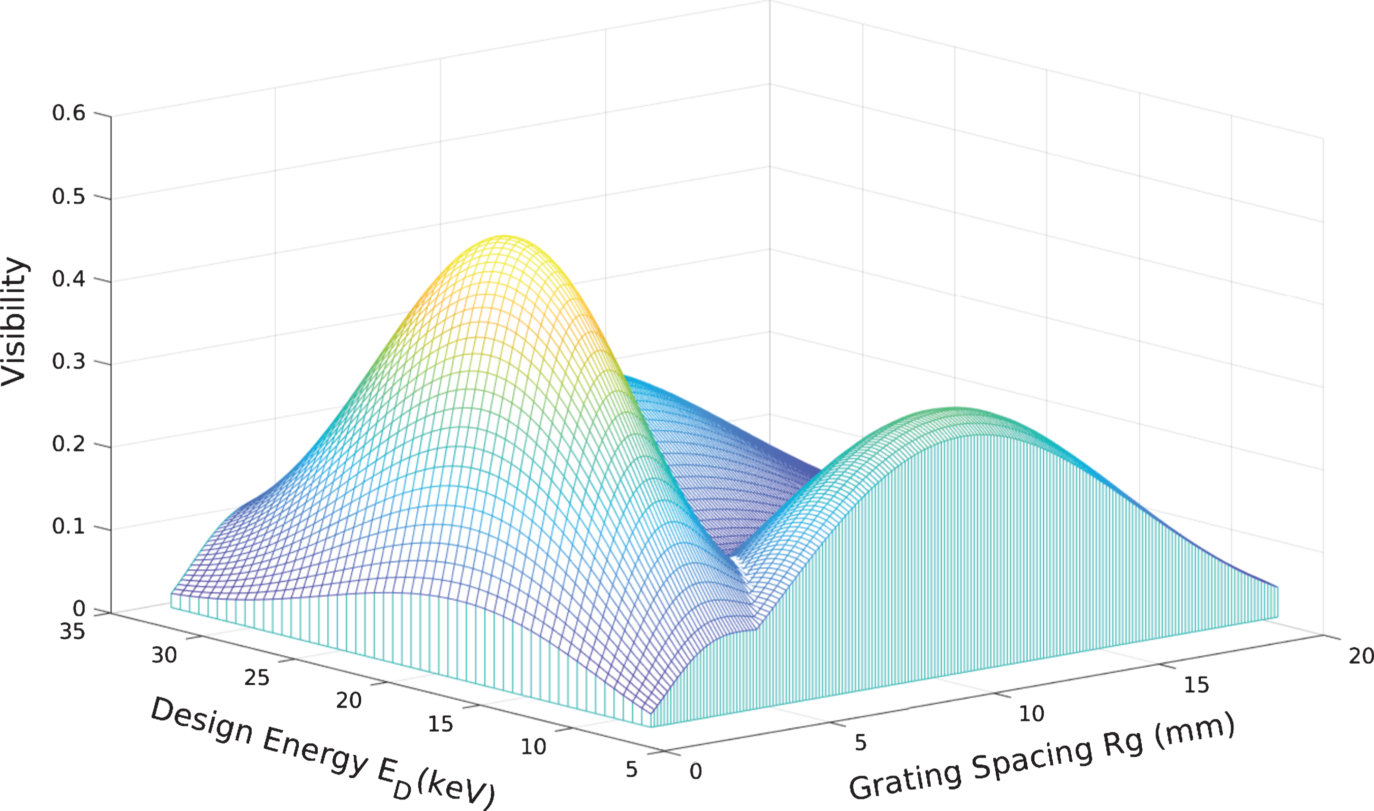
To better understand the relationship between the fringe visibility with respect to grating spacing R_g and gratings’ design energy E_D, we present a mesh plot of the fringe visibility as a function of R_g and E_D as is shown in Fig. 4. In this study, the setups of R_s, R_d, p₁, p₂ as well as the X-ray spectrum are the same as in Fig. 3, and the two gratings have a π-shift at the corresponding design energy E_D ranging from 7.5 keV to 34.5 keV. The grating spacing R_g spans from 1 mm to 20 mm. As can be seen, the fringe visibility peaks at R_g ≈ 3.5 mm and E_D is approximately 20 keV (a position where most of the X-ray is distributed). Therefore, in practice, a grating of a design energy close to the peak of the X-ray’s spectral distribution is preferred. However, the selected grating spacing, R_g controls the fringe period. Therefore, it relies on the detector-pixel size. With this consideration, it can be determined from Fig. 4 that R_g = 3.5 mm, and E_D = 20 keV are optimal configurations.

Fig. 4

Mesh plot of the fringe viability with respect to the grating spacing, R_g, and the gratings’ design energy, E_D. In this simulation, the selection of R_s, R_d, p₁, p₂ are the same as in Fig. 3 with the same X-ray spectrum as shown in Fig. 2. For details, see text.

Another popular choice of phase gratings is the π/2-shifting grating. We now consider a dual-phase grating interferometer with an identical setup as that described in above example, except that the two phase gratings are both π/2 gratings. Figure 5 shows the calculated V₁ and V₂ as functions of the grating spacing R_g. The green-dashed curve plots V₁ and the red-dashed curve plots V₂ as functions of R_g. The solid blue curve in Fig. 5 plots the visibility curve, V = (max(I) - min(I))/(max(I) + min(I)), calculated from Eq. (11-formula). In contrast to the case of the two π gratings, Fig. 5 shows V₁ ⪢ V₂ for R_g values ranging from 6 mm to 16 mm. Therefore, in this range of R_g values, the fringe visibility is equal to the corresponding V₁ values in a good approximation. As shown in Fig. 5, the fringe visibility peaks at approximately 30% for the R_g values ranging from 8 mm to 12 mm. In this range of R_g values, the fringe periods, p_fr, range from 76 – 113.5μm. Nevertheless, for the R_g values ranging from 1 mm to 4 mm, V₂ is larger than V₁, and both V₁ and V₂ are small. This range of the R_g values is not a good choice for the π/2-grating based on the dual grating interferometer.

Fig. 5

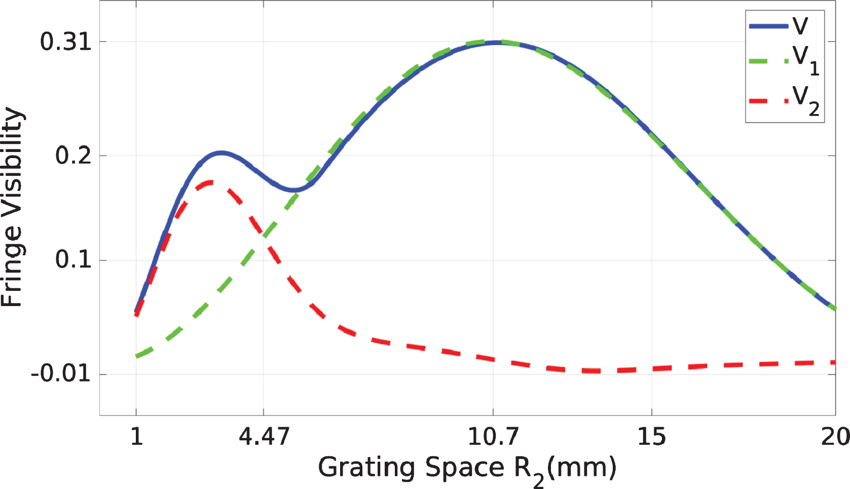
Plot of visibility coefficients V₁, V₂, and fringe visibility V with respect to the G₁-G₂ spacing R_g for dual-π/2 phase gratings. The same set up as in Fig. 3 is assumed, except that the dual π-gratings are replaced with the π/2-gratings. The green curve is the change in the coefficient V₁ with respect to the G₁-G₂ spacing R_g. The red curve is that of V₂. The calculated visibility, V = (max(I) - min(I))/(max(I) + min(I)), based on Eq. (11-formula) is also plotted as the solid blue curve in Fig. 5. In contrast to Fig. 3, the visibility is dominated by V₂ when R_g < 4 mm. When R_g > 5 mm, the visibility is dominated by V₁.

4 Discussion and conclusions

As shown in the previous sections, in contrast to the Talbot–Lau X-ray interferometry, the dual-phase grating interferometry enables the use of a common image detector for the directly resolving the intensity fringes generated by the fine-pitch gratings without the need of absorbing the grating and keeping its system length in check. Removing the absorbing grating with a high-aspect ratio resolves the challenge in grating fabrication and enables the radiation dose reduction by a factor of two. In addition, with this new technique, one can conveniently adjust the fringe period and fringe visibility with almost no change in the total system length. The features of dose saving and system compactness are both critical for future application of grating-based X-ray interferometry in medical imaging.

To facilitate the implementation of this new technique of X-ray interferometry, one needs to quantitatively know how to control the intensity fringe periods, achieve a high fringe visibility with a polychromatic X-ray, and compute a sample’s phase gradients from the measured fringe shifts. The fringe visibility is a figure of merit for the interferometer’s performance. A high fringe visibility reduces the quantum noise in the differential phase images, and increases the interferometry sensitivity. In practice, it is desirable to have explicit expressions of the fringe visibility for systems with phase gratings of any phase modulation and X-ray spectrum. In this study, Eqs. (11) and (11-formula) provide the fringe visibility formulas for the setups with two identical phase gratings with any geometric configuration and any X-ray spectrum of the interferometers. These formulas also incorporate the effect of the focal spot size and detector-pixel size on fringe visibility. As shown in Fig. 3, a numerical simulation of the fringe visibility with a dual π-grating interferometer validates our formula for the fringe visibility of Eqs. (11) and (11-formula). These formulas provide a useful tool for design optimization of dual-phase grating interferometers.

The fringe visibility in dual phase grating interferometry varies significantly with G₁-G₂ spacing and X-ray spectrum. Fig. 3(b) shows that, the peak fringe visibility is 0.51 for the π-gratings setup studied. But for π/2-gratings setup studied in Fig. 5, the peak fringe visibility is 0.31. One thing is sure, the peak fringe visibility should be lower than that with Talbot-Lau interferometer. This is understandable from our formulas of Eq. (5). In Talbot-Lau interferometry fringe visibility is proportional to C₁ (for a π/2-grating) or C₂ (for a π-grating). But in dual phase grating interferometry, as is shown in Eq. (5), fringe visibility is proportional to C₁ × C_-1 (for π/2-gratings), or proportional to C₂ × C_-2 (for π-gratings). These C_m coefficients are given in Eq. (7), their magnitude are always less than 1. Therefore, the peak fringe visibility in dual phase grating interferometry should be lower than that with Talbot-Lau interferometer. In literature there is a report on fringe visibility in dual phase grating interferometry [27], but it is hard to compare that result to ours, because the interferometer setups are completely different. We hope our work will stimulate more experimental studies on dual phase grating X-ray interferometry.

In addition to the formulas for quantitative analysis of fringe visibility, this study also reveals several implications of X-ray polychromaticity of fringe visibility. As shown in Fig. 3, the most convenient way to adjust the fringe visibility is to simply tune the grating spacing R_g. Figure 3(b) shows that the achievable fringe visibility is only moderately reduced compared to the monochromatic X-ray setups, provided that the grating spacing, R_g, is properly set. In contrast, in the Talbot–Lau grating interferometry, the fringe contrast can be reversed by the polychromaticity of the setups with π/2 phase gratings. Such a reversal in the fringe contrast can cause cancellation and a significant reduction in the fringe visibility for the Talbot–Lau interferometry with the polychromatic X-ray [28]. Furthermore, as shown in Fig. 4, the grating design energy, compared to the average photon energy of the X-ray beam, has a significant effect on the fringe visibility. In practice, the probable range of the average photon energy of the X-ray beam can be easily approximated. Figure 4 shows that, for a good fringe visibility, one should select the phase gratings with a design energy that falls into this range. If it is infeasible to make the “match”, one should select the phase gratings with a design energy that is lower, rather than one that is higher than the average photon energy as suggested by Fig. 4.

In conclusion, this study, presents a general quantitative theory of a dual-phase grating X-ray interferometry. The theory provides explicit expressions that predicts the fringe visibility in the dual-phase grating X-ray interferometry. The derived formulas are applicable to the setup with phase gratings of any phase modulation with either monochromatic or polychromatic sources. Numerical simulations are presented to validate the derived formulas. The theory provides a useful tool for design optimization of dual phase grating X-ray interferometers.

Funding

National Institute of Health (NIH) (1R01CA193378).

References

Momose

, Kawamoto

, Koyama

, Hamaishi

, Takai

and Suzuki

, Demonstration of x-ray talbot interferometry, Japanese Journal of Applied Physics 42 (2003), L866–L868.

Weitkamp

, Diaz

, David

, Pfeiffer

, Stampanoni

, Cloetens

and Ziegler

, X–ray phase imaging with a grating interferometer, Optics Express 13 (2005), 6296–6304.

Momose

, Recent advances in x-ray phase imaging, Japanese Journal of Applied Physics 44 (2005), 6355–6367.

Pfeiffer

, Weitkamp

, Bunk

and David

, Phase retrieval and differential phase-contrast imaging with low-brilliance x-ray sources, Nature Physics 2 (2006), 258–261.

Yashiro

, Terui

, Kawabata

and Momose

, On the origin of visibility contrast in x-ray talbot interferometry, Optics Express 18 (2010), 16890–16901.

Zhu

P.P.

, Zhang

, Wang

Z.L.

, Liu

Y.J.

, Liu

X.S.

, Wu

Z.Y.

, McDonald

S.A.

, Marone

and Stampanoni

, Low-dose, simple, and fast grating-based x-ray phase-contrast imaging, Proceedings of the National Academy of Sciences, USA 107 (2010), 13576–13581.

Bevins

, Zambelli

, Li

, Qi

and Chen

G.-H.

, Multicontrast x-ray computed tomography imaging using talbot-lau interferometry without phase stepping, Medical Physics 39 (2012), 424–428.

Tang

, Yang

and Tang

, Characterization of imaging performance in differential phase contrast ct compared with the conventional ct: Spectrum of noise equivalent quanta neq(k), Medical Physics 39 (2012), 4367–4382.

Teshima

, Setomoto

and Den

, Two-dimensional gratings-based phase-contrast imaging using a conventional x-ray tube, Optics Letters 36 (2011), 3551–3553.

10.

Bennett

, Kopace

, Stein

and Wen

, A grating-based single shot x-ray phase contrast and diffraction method forimaging, Medical Physics 37 (2010), 6047–6054.

11.

Jiang

, Wyatt

and Wang

, X-ray phase-contrast imaging with three 2d gratings, International Journal of Biomedical Imaging, pages 827152–927159, 2008.

12.

Itoh

, Nagai

, Sato

, Yamaguchi

, Nakamura

, Kondoh

, Ouchi

, Teshima

, Setomoto

and Den

, Two-dimensional grating-based x-ray phase-contrast imaging using fourier transform phase retrieval, Optics Express 19 (2011), 3339–3346.

13.

Bravin

, Coan

and Suortti

, X-ray phase-contrast imaging: from pre-clinical applications towards clinics, Physics in Medicine and Biology 58 (2013), R1–R35.

14.

Momose

, Kuwabara

and Yashiro

, X-ray phase imaging using lau effects, Applied Physics Express 4 (2011), 066603.

15.

Morimoto

, Fujino

, Ohshima

, Harada

, Hosoi

, Watanabe

and Shimura

, X-ray phase contrast imaging by compact talbot-lau interferometer with a single transmission grating, Optics Letters 39 (2014), 4297–4300.

16.

Morimoto

, Fujino

, Yamazaki

, Ito

, Hosoi

, Watanabe

and Shimura

, Two dimensional x-ray phase imaging using single grating interferometer with embedded x-ray targets, Optics Express 23 (2015), 16582–16588.

17.

Yan

, Wu

and Liu

, A general theory of interference fringes in x-ray phase grating imaging, Medical Physics 42(6) (2015), 3036–3047.

18.

Yan

, Wu

and Liu

, Predicting visibility of interference fringes in x-ray grating interferometry, Optics Express 24 (2016), 15927–15939.

19.

Yan

, Wu

and Liu

, Polychromatic x-ray effects on fringe phase shifts in grating interferometry, Optics Express 25 (2017), 6053–6068.

20.

Yan

, Wu

and Liu

, Beam hardening correction in polychromatic x-ray grating interferometry, Optics Express 25 (2017), 24690–24704.

21.

Donath

, Chabior

, Pfeiffer

, Bunk

, Reznikova

, Mohr

, Hempel

, Popescu

, Hoheisel

, Schuster

, Baumann

and David

, Inverse geometry for grating-based x-ray phase-contrast imaging, Journal of Applied Physics 106 (2009), 054703.

22.

Miao

, Panna

, Gomella

, Bennett

, Znati

, Chen

and Wen

, A universal moiré effect and application in x-ray phase-contrast imaging, Nature Physics 12 (2016), 830–836.

23.

Kagias

, Wang

, Jefimovs

and Stampanoni

, Dual phase grating interferometer for tunable dark-field sensitivity, Applied Physics Letters 110(6) (2017), 014105.

24.

Yan

, Wu

and Liu

, Quantitative theory of x-ray interferometers based on dual phase grating: fringe period and visibility, Optics Express 26 (2018), 23142–23155.

25.

, Chen

, Zhu

, Yang

, Deng

, Shi

, Zhang

, Guo

, Zhang

, Zheng

and Liang

, Dual phase grating based x-ray differential phase contrast imaging with source grating: theory and validation, Optics Express 28 (2020), 9786–9801.

26.

Yan

, Wu

and Liu

, Clarification on generalized lau condition for x-ray interferometers based on dual phase gratings, Optics Express 27(16) (2019), 22727–22736.

27.

Bopp

, Ludwig

, Seifert

, Pelzer

, Maier

, Anton

and Riess

, Simulation study on x-ray phase contrast imaging with dual-phase gratings, International Journal of Computer Assisted Radiology and Surgery 14(1) (2019), 3–10.

28.

Hipp

, Willner

, Herzen

, Auweter

, Chabior

, Meiser

, Achterhold

, Mohr

and Pfeiffer

, Energy-resolved visibility analysis of grating interferometers operated at polychromatic x-ray sources, Optics Express 22 (2014), 30394–30409.