Comparison of irregular flux viewer system with BONENAVI version for identification of Tc-99m MDP whole body bone scan metastasis images

Abstract

The Tc-99m methylene diphosphonate (MDP) whole body bone scan (WBBS) has been widely accepted as a method of choice for the initial diagnosis of bone and joint changes in patients with oncologic diseases. The WBBS has shown high sensitivity but relatively low specificity due to bone variation. This study aims to use the self-developing irregular flux viewer (IFV) system to predict possible bone lesions in planar WBBS. The study uses gradient vector flow (GVF) and self-organizing map (SOM) methods to analyze the blood fluid-dynamics and evaluate hot points. The evaluation includes a selection of 368 patients with bone metastasis from prostate cancer, lung cancer and breast cancer. Finally, we compare IFV values with BONENAVI version data. BONENAVI is a computer-assisted diagnosis system that analyzes bone scintigraphy automatically. The analysis shows that the IFV system achieves sensitivities of 93% for prostate cancer, 91% for breast cancer, and 83% for lung cancer, respectively. On the other hand, our proposed approach achieves a higher sensitivity than the results of BONEVAVI version 2.0.5 for prostate cancer (88%), breast cancer (86%) and lung cancer (82%), respectively. The study results demonstrate that the high sensitivity and specificity of the IFV system can provide assistance for image interpretation and generate prediction values for WBBS.

Keywords

Tc-99m MDP irregular flux viewer (IFV)computer-aided diagnosis (CAD)whole body bone scan (WBBS)machine learning (ML)

1 Introduction

The morbidity and mortality rates of cancer are increasing worldwide, and more than 12 % of men and 10% of women may develop the disease eventually due to the accumulation of risks [1]. The skeletal system is one of the most common sites of distant metastasis in many cancers [2], especially in breast, prostate and lung cancers, which are known for their high incidence rate of bone metastasis. Currently, the Whole-Body Bone Scan or bone scintigraphy (BS), which is widely accepted as a method of choice for the initial diagnosis of bone and joint changes in patients with oncologic diseases [3 –6], is a well-known clinical routine investigation and one of the most frequent diagnostic procedures in nuclear medicine. Indications for BS include benign and malignant diseases, infections, degenerative changes and others [7]. Furthermore, BS has high sensitivity, and the changes of the bone metabolism are seen earlier than changes in bone structure detected on radiograms [8]. Despite the advent of various imaging modalities, whole-body scintigraphy remains the standard method for surveying the existence and extent of skeletal metastasis. The interpretation of BS is performed visually and requires experience due to the difficulties associated with pattern recognition [9]. The adjustment of brightness and contrast in nuclear medicine Whole Body Bone Scan (WBBS) images may confuse nuclear medicine physicians when identifying small bone lesions and may make identifying subtle bone lesion changes in sequential studies difficult [10]. Therefore, an appropriate quantitative approach is required for bone scintigraphy interpretation [9].

Tc-99m methylene diphosphonate (99mTc MDP) WBBS is used to evaluate skeletal diseases in nuclear medicine. It presents good imaging modalities in several bone diseases, for example, bone metastasis, primary bone tumor or bone trauma [11]. In general, there are two reactions in bone metabolism: one is the osteoblastic reaction, and the other is the osteoclastic reaction. These are balanced under normal physiological conditions. If a trauma of the bone occurs, it will induce an osteoblastic reaction. Calcium and phosphate ions participate in osteoblastic reactions and are also used for monitoring bone condition. The radiotracer can be combined with MDP, which is injected intravenously into the body. After that, MDP will attach to the mineral substance of the bone, presenting a different focal uptake, which will be acquired by a gamma camera [12]. When distributed MDP gathers, it reveals a hot point (or specific point) in the bone scan, and this is helpful for physicians to evaluate a bone abnormality. In 1998, a study indicated that 99mTc MDP WBBS could be used for the long-term follow-up of bone metastasis or primary bone tumors. Currently, computer-aided diagnosis (CAD) systems have become important; the application of medical imaging is also becoming increasingly important [13, 14]. However, currently, the use of computer-aided diagnostic WBBS images in nuclear medicine is still quite limited. In 2004, Yin and Chiu et al. studied the use of technology to develop a fuzzy inference applied to planar bone scan images of a CAD system [15].

On the other hand, the standard diagnostic method since the 1970s has been planar or Single photon Emission Computed Tomography (SPECT) scintigraphy using 99mTc-labeled polyphosphonates. Studies by Schirrmeister et al. demonstrated that planar BS was 80–90% sensitive in the detection of peripheral skeletal metastases but as low as 20–40% sensitive in the detection of vertebral metastases [16]. A CAD scheme, termed the irregular flux viewer (IFV) and based on gradient vector flow [17 –20] was developed. Patients’ images were examined to improve the limitation of BS. In this study, we aimed to determine how to increase the visual quality to identify the correlation between WBBS by IFV and magnetic response images (MRI) or computerized tomography (CT) for bone metastasis. We also aimed to evaluate the clinical value of 99mTc MDP WBBS compared with the results of staging in prostate cancer, breast cancer and lung cancer. By determining the indicator in prostate cancer, breast cancer and lung cancer imaging, morbidity and mortality may be improved.

First, we attempted to develop a ML (machine learning) interface using the Gradient Vector Flow (GVF) scheme to assist in the calculation of a characteristic index of the blood fluid-dynamic analysis, which includes the first to third gradient index and a dynamic index. Then, we proposed another view-tool scheme, termed IFV, for the evaluation of the hot points based on self-clusters and union clusters to improve the accuracy of the method. It was shown that the proposed method achieved better metastasis prediction performance than traditional images.

2 Material and methods

2.1 Set of WBBS database for ML resource

Patient Population: This study was a retrospective study. The study was retrospectively choosing 106 data sets of prostate cancer, 100 data sets of breast cancer and 162 of lung cancer, following both Tc-99m MDP WBBS and MRI scans (or CT scans). Different populations of males and females were included from August 2011 to August 2014.

Equipment, Energy Window and Simulation Environment: Gamma camera: Philips (Brightview) & Siemens SPECT/CT scanner (Symbia T); Collimator: Low Energy General Purpose (LEGP) or Low Energy All Purpose (LEAP); Matrix size: 512×1024 (Whole Body); Energy window: 140 Kev, 15%; Whole Body Speed: 20 cm/min. In our work, Matlab8.1 (R2013a) or SPSS statistics were selected to calculate parameters such as receiver operating characteristic curves (ROC), self-organizing map (SOM) statistics or the centroid method for cluster analysis in order to distinguish the correlation and difference between the parameters of the mean, SD and entropy in the WBBS, MRI, SPECT/CT and PET/CT scans for metastasis. The developed CAD scheme is clinically helpful and makes it easier to perform early detection and discrimination.

WBBS Imaging Procedure and Principal: To help diagnose the pathology of the skeletal system, patients were injected with radiopharmaceuticals composed of 20 mCi 99mTc MDP and a bone-seeking molecule, such as analogs of calcium, hydroxyl groups or phosphates. In fact, the most commonly used molecule for this is organic diphosphonate bound to Tc-99m. The Tc-99m methylene diphosphonate (MDP) Whole Body Bone Scan (WBBS) images of patients were then scanned by a gamma camera 2–4 h later; typically, both anterior and posterior scans were taken (Fig. 1). The mechanism behind the uptake of the radio-diphosphate is chemisorption (which is the adsorption of a molecule to a surface based on chemical bond formation) on the surface of hydroxyapatite crystals of the bone matrix. The determinant of increased uptake is increased skeletal metabolic activity (primarily, the extent of osteoblastic activity), and accounting for increased uptake at growth centers and centers of osteoblastic and other metabolic activity, increased blood flow and a loss of sympathetic tone causes vascular dilatation and hyperemia [16].

Classification of WBBS Database and Imaging Processing: First, Digital Imaging and Communications in Medicine (DICOM) viewer software was used to transform the original WBBS DICOM images to JPG. According to NM WBBS clinical diagnostic reports, the sample was divided into a four-group patient database of cancer types including no metastasis, degenerative change (DJD), mild metastasis and severe metastasis from prostate cancer, breast cancer and lung cancer. Then, images were examined by the CAD scheme, and the ML interface was searched for the gradient and dynamic index; furthermore, irregular flux points and clusters were evaluated by the IFV software (Fig. 2). Finally, the results were combined with the images of the WBBS and MRI scan (or CT scan) for bone metastasis following prostate cancer, breast cancer and lung cancer. Otherwise, the CAD scheme would be respectively analyzed by Matlab 8.1 in terms of different features, including metastasis size, localization, critical period, etc. The machine learning (ML) architecture is illustrated in Fig. 3 [17].

Fig. 1

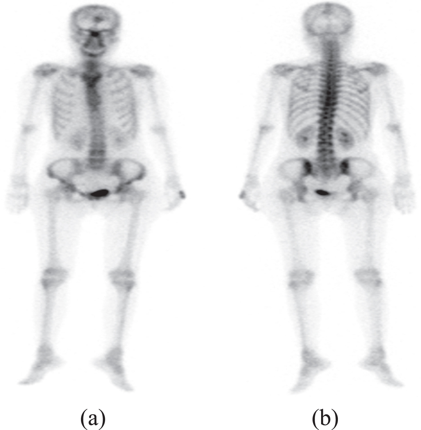
Tc-99m methylene diphosphonate (MDP) Whole Body Bone Scan (WBBS) images in (a) anterior view and (b) posterior view.

Fig. 2

Machine learning (ML) interface using the Gradient Vector Flow (GVF) scheme to assist in the characteristic index of the blood fluid-dynamic analysis, which includes the first to third gradient value and dynamic value.

Fig. 3

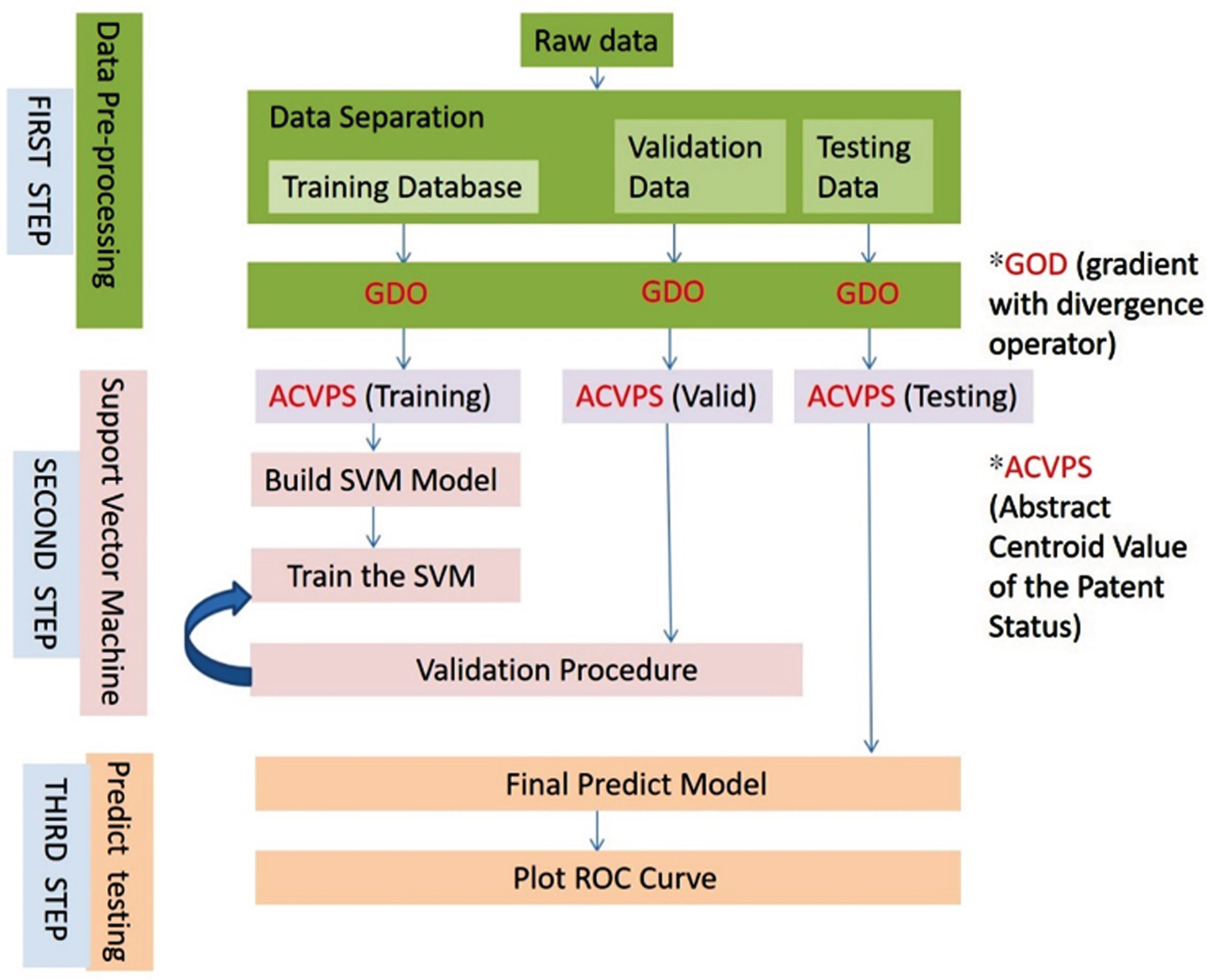
Illustration of ML architecture used in this study.

Traditionally, nuclear medicine studies determine the state of an illness by using the image pixel from the instrument directly. The inspectors adjust the brightness and the contrast of the infection images, helping doctors to assess the instant status of the patients by the shade of the image only. This method does not reveal important information hidden in the pixels of the BS images. It is known that radiopharmaceuticals are transferred by the blood arteries and veins; thus, the blood flow status corresponds to the spatial change of the image pixel. The developments of tumors often accompany an irregular quantity of the blood sink/source or artery/vein growth. To study the feature of irregular flux regarding the blood flow, this study designed a simple algorithm for the software to view the irregular flux hot points and then suggested hot points in which tumors could be located.

2.2 Gradient vector flow (GVF)

A vector field refers to each point (x, y, z) within a region and corresponds to the relationship between vectors. In other words, the vector field is a vector function of three variables. Any component of a vector field can be presented as follows: $\vec{F} (x, y, z) = F_{1} (x, y, z) i + F_{2} (x, y, z) j + F_{3} (x, y, z) k$ (1)

$\vec{F} (x, y, z)$ is assumed to be defined in the space of a region if any are related; every point through the tangent with $\vec{F}$ to the curve in this area is called the flow line or stream line of this curve or characteristic curve. A vector field determines the direction of each point in a region. If there is particle motion in this region that is consistent with the position in the direction of the vector field in the direction of the velocity at any position, the particle ‘s trajectory follows the flow-line. Since the direction of the flow-line is uniquely determined by the vector field, the two flow-lines cannot intersect. If the space of some of the points of the vector field is zero, these points have no direction at all, so there will not be flow-lines through these points.

Assume that $\vec{R}$ is the position of any point on the vector flow line, and the length of the line along flow path s refers to the metrics; then, the unit tangent to the vectors of the flow line is

$\frac{df}{ds} = \frac{\partial f}{\partial x} \frac{dx}{ds} + \frac{\partial f}{\partial y} \frac{dy}{ds} = \frac{\partial f}{\partial x} cos α + \frac{\partial f}{\partial y} sin α = (\frac{\partial f}{\partial x}, \frac{\partial f}{\partial y}) \cdot (cos α, sin α) = \nabla f \cdot \vec{T}$ (2)

Because each point is tangential to the vector field flow lines, it should have the same direction; that is,

$\vec{T} = β \vec{F} \Rightarrow β F_{1} = \frac{dx}{ds}, β F_{2} = \frac{dy}{ds}, β F_{3} = \frac{dz}{ds} \Rightarrow \frac{dx}{F_{1}} = \frac{dy}{F_{2}} = \frac{dz}{F_{3}}$ (3)

This equation is called the flow-line equation [16 –18].

The divergence of a vector field $\vec{F} (x, y, z) = F_{1} (x, y, z) i + F_{2} (x, y, z) j + F_{3} (x, y, z) k$ is defined as $div \vec{F} = \nabla \cdot \vec{F} = \frac{\partial F_{1}}{\partial x} + \frac{\partial F_{2}}{\partial y} + \frac{\partial F_{3}}{\partial z}$ (4)

The physical meanings of divergence and curl principles are also explored in hydrodynamics. Otherwise, the divergence of a vector field is converted to a scalar field. A curl will convert a scalar field to a vector field.

2.3 Self-organizing map (SOM)

The Self-Organizing Map (Self-Organizing Feature Maps) network (generally referred to as SOFM or SOM) is based on a network performing “competitive learning”, which means that their output neuron layers compete with each other to fight to achieve the activation of opportunity. Self-Organizing Maps are different from other artificial neural networks in the sense that they use a neighborhood function to preserve the topological properties of the input space. Competitive learning is essentially a self-organizing learning approach; its basic concept is the use of unlabeled samples to find some similar characteristics, rules or relationships. Common characteristics of the samples are gathered into the same kind.

The ML method with competitive learning is sometimes called “winner-take-all” learning, which was introduced by the Finnish professor Teuvo Kohonen in the 1980s [21, 22]. In an actual network, the lateral inhibition architecture was utilized to achieve this objective. Lateral inhibition operates mainly by the interaction of neurons in the output to find the maximum value that builds on the work of biological neural models from the 1970s [23] and morphogenesis models dating back to Alan Turing in the 1950s [24].

However, an unsupervised learning network is a network using an artificial intelligence algorithm, which aims to classify raw data in order to understand the internal structure of materials [25]. Unlike network-supervised learning, unsupervised learning networks do not know if their classification results are correct, as it is not provided with supervised enhancement (to tell it what kind of learning is correct). Its inputs are only examples of such a network, and it will automatically find its underlying rule categories from these examples. When the study is completed and after the test, the network can also be applied to new cases.

SOM was proposed by Kohonen in 1982 with the aim of using a lower-dimensional topology map to visualize the high-dimensional information of certain cases. It belongs to the category of feedforward, unsupervised learning networks, and the network is trained simultaneously in a competition pattern [26]. A characterized paradigm can enter the learning process, resulting in self-organization and the need to rely on the target output value and perform the correction of errors. SOM can also show the distribution of the input sample or similarity, and it has good ability to emerge and classify cases into a set of clusters into groups with similar properties [27].

2.4 Irregular flux viewer (IFV)

The IFV method has some disadvantages, including that (1) the analysis algorithm was not suitable for pediatric patients because the gray level distribution in the joint area of children is higher than adults—thus, another database of bone gray level uptake in bone images of pediatric patients has to be constructed—and that (2) the other approach is not suitable for “cold” lesion detection. In the case of artificial joint replacement and bone necrosis, the calculation of the algorithm missed lesions.

A few further works may continue the use of the proposed approach. Here, a set of possible cases which may be regarded as open and valuable problems to be researched are as follows: (1) the building of a database that is suitable for patients of all ages, solving the problem of the limitation of our algorithm to adults only; and (2) the development of another analysis algorithm to detect “cold” bone lesions. The method of the irregular flux viewer (IFV) (Figs. 4 and 5) is described in two parts: the definition of the blood fluid-dynamics analysis and the evaluation of the hot points.

Fig. 4

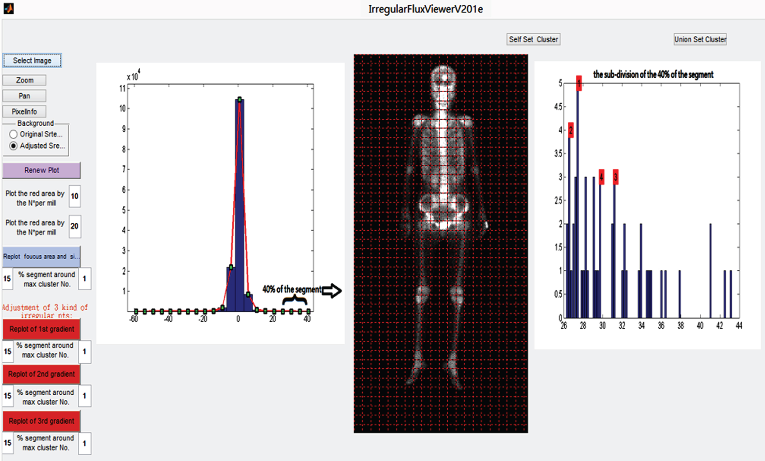
Irregular flux viewer (IFV) interface: searching for the irregular flux points (left) and cluster analysis by histogram distribution (right).

Fig. 5

Irregular flux viewer (IFV) interface: definition of characteristic points.

2.4.1 Analysis: The definition of the blood fluid-dynamics

In this study, the pixel image was seen as the scalar potential field and introduced the gradient and divergence definition to calculate the quantity value of sink/source about every pixel grid. According to vector calculus of the fluid field [28, 29], the gradient definition is a generalization of the usual concept of a derivative of a function in one spatial dimension to a function in two or several spatial dimensions. It gives the maximum flow value and direction of every pixel grid.

The gradient operator is given in the below formula: $\nabla φ = (\frac{\partial φ}{\partial x} \vec{i}, \frac{\partial φ}{\partial y} \vec{j})$

where φ is the pixel image of bone scan. This can be written in a matrix discrete form: $\begin{matrix} \nabla φ (i, j) & = (\frac{φ (i, j) - φ (i - 1, j)}{i - (i - 1)} \vec{i,} \frac{φ (i, j) - φ (i, j - 1)}{j - (j - 1)} \vec{j}) \\ = (φ (i, j) - φ (i - 1, j), φ (i, j) - φ (i, j - 1)) \end{matrix}$

The study was obtaining the flow status of a grey image by calculating its spatial difference of the i and j index, which increases along with x and y direction from the left top of the image.

When the flow vector field of a bone scan images were obtained, the sink/source points could be counted by the definition of the divergence.

The operator of the divergence is $div \vec{A} = \nabla \cdot \vec{A} = \frac{\partial P}{\partial x} + \frac{\partial Q}{\partial y}$

where A is the vector field of the flow i.e., It can be written in the discrete form as $div A (i, j) = \frac{P (i, j) - P (i - 1, j)}{i - (i - 1)} + \frac{Q (i, j) - Q (i, j - 1)}{j - (j - 1)}$

If the vector field of the flow (i.e., the gradient vector field of the bone scan image) was introduced, it would obtain the sink/source of every pixel grid, which indicates the total income/outcome. The gradient-divergence analysis that led to the sink/source analysis could be expressed in the difference form of pixel value as in the following: $\begin{matrix} \nabla \cdot (\nabla φ (i, j)) = φ (i, j) - 2 φ (i - 1, j) + φ (i - 2, j) \\ + φ (i, j) - 2 φ (i, j - 1) + φ (i, j - 2) \end{matrix}$

This difference value method of image processing is the kernel of the algorithm of the IFV software. It can give the relative quantity analysis of patient image that is more robust and objective than the image processed by the inspectors adding the brightness and the contrast only.

2.4.2 Evaluation of the patient’s hot point detection

Here, the working processes of software are described and discussed.

Step 1: The original DICOM file was transferred to the JPG file and then read to do the gradient-divergence analysis to obtain the sink/source of every pixel image. If the spatial total (i.e., the divergence) of the x and y directional flow of the potential (i.e., the gradient of the bone scan image) was positive, the image grid was called the sink; otherwise, the image grid was called the source. The location of the maximum sink showed the possibility growth point of cancer or inflammation because the cancer metastasis/ inflammation needed a lot of the nutrition given by the blood transport.

Step 2: Using the result images of the Step1 repeated the calculation of the Step1 again. It could obtain the so-called the sink/source of the sink/source. It was a kind of generalized velocity of the sink/source obtained in Step1. It shows the velocity tendency of the radiopharmaceuticals being transferred by the blood that also reflects the nutrition.

Step 3: The result images of the Step2 repeated the calculation of the Step1 itself once again. It was a kind of generalized force of the sink/source obtained in Step1. The calculation goal was the same as in Step2. The kernel idea of this study was to find the irregular flux status of the absorbing nutrition given by the blood circulation.

Step 4: This study defined the top 40% division part of the histogram about the image grid quantity counting in the Step1 to 3 results showed being irregular flux occurring. As (Fig. 4 (left)) shows, the histogram was counted in twenty-one divisions between its maximum and minimum. The minimum is located in the left boundary of the first division and the maximum is located in the right boundary of the twenty-one divisions. So, the eleventh division was the median number locations, which counted the zero and almost zero image grids. Then, each of the negative and the positive sink/source, velocity, and force value had ten counting divisions within the histogram. This study defined 18th and 21st divisions as the irregular flux occurring division. These were the so-called the top 40% irregular divisions.

Step 5: The goal of step 5 was to find the hot points in the top 40% irregular divisions. The irregular divisions were re-divided into fifty divisions and find the hot points by the maximum counting value in these new sub-divisions of histogram (Fig. 4 (right)). This study also provided the second, third, and fourth maximum counting value for the other hot point choices. To get the suitable numbers of the hot points for visualization, the range unit of sub-division could be adjusted from 15% to 50% to mark the hot points that had the values located in the range describing in the above.

Step 6: The top 10% non-zero total image grids of the original intensity JPG were defined as the red area, and the top 10% ∼20% non-zero ones were defined as the blue area (Fig. 5 red circle). The goal of this step was to plot the blue area and red area with the hot points in advantage of the original intensity JPG as the base map (see red & blue arrow). Comparing the base map and the hot point’s location would tell us the serious area/points where metastases may occur.

2.5 Overview of the application of our research design

As mentioned above, the gradient only calculates the variation of the radiotracer blood-flowing input (sink) or output (source) of the local point; however, we aimed to calculate the quantity value of the sink/source for every pixel grid. The gradient definition is a generalization of the usual concept of a derivative of a function in one spatial dimension to a function in two or more spatial dimensions. In order to determine the impact of the inflow or the outflow, another definition of vector field analysis was introduced. First, there must be a flow of information to provide a vector field, which is the last section of the gradient field: $div \vec{A} = \nabla \cdot \vec{A} = \frac{\partial P}{\partial x} + \frac{\partial Q}{\partial y}$

The values were calculated gradient and divergence in each image acquisition. This is so called the changes of each pixel in image during in and out phases of the radiotracer activity. After the process, the scalar field was changing to vector field, obtaining another image of in and out phases. This is an inevitable process, but it does not affect the judgment of the image. The vector field of the flow (i.e., the gradient vector field of the bone scan image), it would obtain the sink/source of every pixel grid, which indicates the total income/outcome. The study was try to calculate the index value of gradient and divergence. If the spatial total (i.e., the divergence) of the x and y directional flow of the potential (i.e., the gradient of the bone scan image) was positive, the image grid was called the sink; otherwise, the image grid was called the source.

Finally, to identify index value range of normal and abnormal with the patients, then the calibrated rate of blood flow in and out of a maximum of 15% histogram point abnormal tissues. The kernel idea of this study was to find the irregular flux status of the tumor nutrition absorption round the blood circulation by semi-quantitative method.

Images manifesting the input or output of blood flow (including rate, velocity and force) were compared to the characteristic index, which was calculated and written in function code B. The previously calculated available rate of the three related characteristic index values constituted an abstract space to discriminate the normal and abnormal border areas (Fig. 6). The early diagnosis, treatment, and prevention of the metastasis of tumors to bone lesions is one of the purposes of this study.

Fig. 6

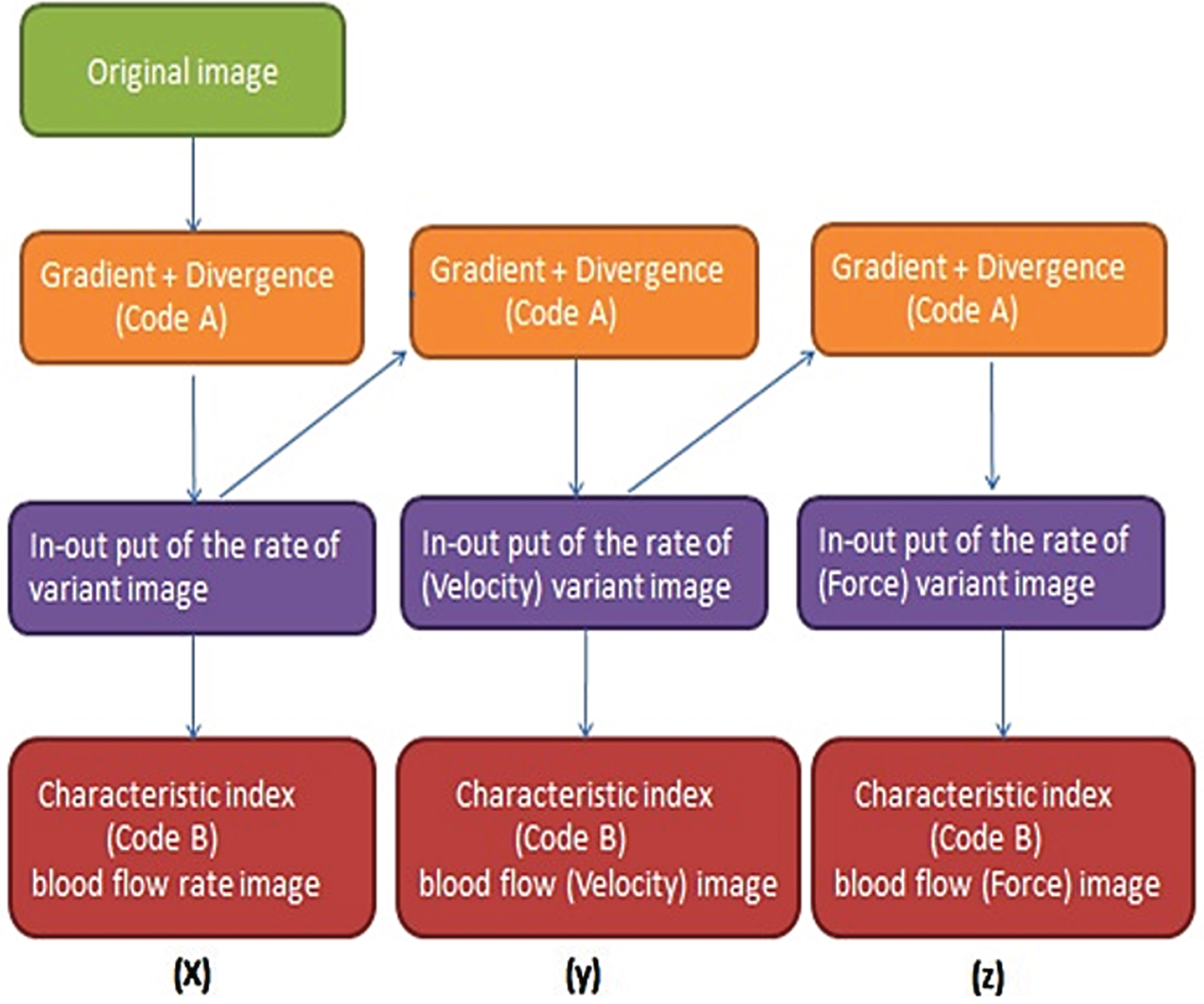
The procedure of our CAD-code design.

3 Results

Our approach is devised with three main steps, which include post-processing, irregular flux points and cluster detecting, and analysis. In the analysis stage, the study was determined the bone lesion threshold by the correction of SD and centroid method cluster classicistic analysis in the WBBS histogram. After experimenting with our algorithm, the performance was evaluated by ROC curve and SOM analysis (Table 1 –3).

Table 1
The analytic results of 106 male prostate cancer patients

Type No Meta. Degenerative Mild Meta. Severe Meta.

Index (40 pts) (17pts) (15 pts) (34 pts)

Gradient (first to third) value (ANT) 29.18 37.70 39.28 48.81

Gradient (first to third) value (POST) 30.33 35.08 38.26 53.53

Dynamic value (ANT) 17.43 22.87 26.79 42.52

Dynamic value (POST) 15.83 24.70 30.13 46.66

Type	No Meta.	Degenerative	Mild Meta.	Severe Meta.
Gradient (first to third) value (ANT)	29.18	37.70	39.28	48.81
Gradient (first to third) value (POST)	30.33	35.08	38.26	53.53
Dynamic value (ANT)	17.43	22.87	26.79	42.52
Dynamic value (POST)	15.83	24.70	30.13	46.66

Gradient value index: No Meta. Range: 29.18-37.70; ^*Meta. Range: 38.26–53.53. Dynamic value index: No Meta. Range: 15.83–24.70; Meta. Range: 26.79–46.66. Prostate Ca. total: 106 male patients (Near normal: 57; Meta.: 49) Mean age = 76.09; SD = 8.98; confidence interval (CI) (95%) = 51.83∼94.05. ANT: anterior view; POST: posterior view.

Table 2

The analytic results of 162 female breast cancer patients

Type	No Meta.	Degenerative	Mild Meta.	Severe Meta.
Index	(33 pts)	(61pts)	(33 pts)	(35 pts)
Gradient (first to third) value (ANT)	33.72	38.92	43.24	42.49
Gradient (first to third) value (POST)	35.37	36.67	39.07	49.24
Dynamic value (ANT)	23.70	29.01	32.42	34.40
Dynamic value (POST)	21.68	26.26	31.01	47.43

Gradient value index: No Meta. Range: 33.72–38.92; Meta. Range: 39.07–49.24. Dynamic value index: No Meta. Range: 21.68–29.01; Meta. Range: 31.01–47.43. Breast Ca. total: 162 female patients (Near normal: 94; Meta.: 67); Mean age = 55.96; SD = 10.16; CI (95%) = 35.64∼76.28.

Table 3

The analytic results of 100 lung cancer patients

Type	No Meta.	Degenerative	Mild Meta.	Severe Meta.
Index	(42 pts)	(13pts)	(15 pts)	(30 pts)
Gradient (first to third) value (ANT)	34.88	35.43	37.53	40.57
Gradient (first to third) value (POST)	36.06	34.30	36.80	48.05
Dynamic value (ANT)	26.37	29.52	33.03	37.76
Dynamic value (POST)	25.25	24.17	23.85	38.60

Gradient value index: No Meta. Range: 34.30–36.06; Meta. Range: 36.80–48.05. Dynamic value index: No Meta. Range: 24.17–29.52; Meta. Range: 23.85–38.60. Lung Ca. total: 100 patients (Near normal: 55 (male:29 and female 26); Meta.: 45 patients (male:24, female:21)). Mean age = 60.83(Male); SD = 12.42; CI (95%) = 35.99 ∼ 85.67. Mean age = 65.84 (Female); SD = 9.95; CI (95%) = 45.94 ∼ 85.74.

In our study, a total of 45.9% of male patients (73/159) and 42.1% of female patients (88/209) exhibited bone metastases. The sensitivity of bone scan reporting when used only to predict skeletal metastasis was better in prostate cancer (89%) than breast cancer (85%) and lung cancer (72%). For prostate cancer, area under the curve (AUC) values were 0.88 (95% confidence interval (CI) 0.87∼0.90), and the SD was 0.13. For breast cancer, the AUC values were 0.85 (95% CI 0.83∼0.86), and the SD was 0.013. For lung cancer, the AUC values were 0.72 (95% CI 0.70∼0.73), and the SD was 0.016. On the other hand, the overall sensitivities of the SOM for prostate cancer showed that the AUC values were 0.81 (95% CI 0.78∼0.84), and the SD was 0.012. For the SOM for breast cancer, the AUC values were 0.64 (95% CI 0.63∼0.64), and the SD was equal to 0.002. Finally, for the SOM for lung cancer, the AUC values were 0.66 (95% CI 0.54∼0.78), and the SD was equal to 0.049. In our previous study, the percentage of patients with lung cancer was high. Lung cancer metastases to bone are predominantly osteolytic (approximately 75%) [30]. Therefore, the performance of bone scans in patients with lung cancer has a low validation rate [31].

On the other hand, comparison of the clinical modalities of MRI, CT, SPECT/CT, and PET/CT with IFV-BS reports was done and a follow-up bone scan and clinical course was performed. Our proposed approach had a higher sensitivity to improvements of the inherent limits of osteolytic lesions in planar bone scintigraphy. The corresponding results show sensitivity to the prediction of skeletal metastasis in prostate cancer (93%), breast cancer (91%) and lung cancer (82%). For prostate cancer, the AUC values were 0.93 (95% confidence interval (CI) 0.92∼0.94), and the SD was 0.0011. For breast cancer, the AUC values were 0.91 (95% CI 0.90∼0.92), and the SD was 0.0016. For lung cancer, the AUC values were 0.83 (95% CI 0.82∼0.84), and the SD was 0.0015.

Furthermore, the overall sensitivities of the SOM for prostate cancer showed that the AUC values were 0.92 (95% CI 0.91∼0.93), and the SD was 0.0046. For the SOM for breast cancer, the AUC values were 0.91 (95% CI 0.90∼0.92), and the SD was equal to 0.005, as shown in Tables 1–3. Finally, for the SOM for lung cancer, the AUC values were 0.83 (95% CI 0.82∼0.84), and the SD was equal to 0.0077. Finally, the lack of metastasis or degeneration was easily discriminated and was under the threshold relative to bone metastasis. Using cluster analysis based on a relative semi-quantification concept, a metastasis area with less than five hot points indicated slight bone metastasis; in contrast, more than five hot points indicate serious bone metastasis. The gradient (first to third) and dynamic statistical values of hot points are helpful in the judgement of whether metastasis has occurred. In summary, the results of our study showed that our abnormal flow browser is reliable and may provide assistance for image interpretation and generate prediction values in WBBS.

4 Discussion

The 99mTc-MDP WBBS shows a high sensitivity but relatively low specificity due to bone variation [32]. While single-photon emission computed tomography (SPECT)/CT could aid in the assessment of suspicious bone metastasis [33], its results are still ambiguous for some lesions [34]. Other radiotracers such as FDG can also be used to detect bone metastasis [35]; however, they are not only expensive, but also subject patients to higher radiation doses. Huang et al. described a computer-aided automatic lesion detection system that is useful and can be used to identify possible bone lesions [10]. The medical image segmentation technique used in medical applications includes quantitative clinical tools for elevating bone metastasis [9 , 36]. Feng et al. demonstrated a model to detect Gradient Vector Flow (GVF) and described a quantitative scheme to detect possible abnormalities [37]. However, osseous metastases are infrequent in endometrial cancer [38]. Bone metastases in endometrial cancer reflect the aggressiveness of the disease [39]. This patient reported not only a rare presentation of bone metastasis in endometrial cancer but also showed disease progression. Even the WBBS revealed a near-normalization of uptake in the T-spine. However, a spinal MRI and biopsy confirmed malignancy. This was supposedly due to osteolytic bone lesions over the T-spine that could be detected by IFV. Otherwise, CT results can classify skeletal metastasis type as osteoblastic, osteolytic, mixed (osteoblastic and osteolytic) and intertrabecular. In the early stage of skeletal metastasis, when cancer cells reach the bone marrow and spread within the bone marrow space (intertrabecular space), the changes in the bone are minimal. Therefore, CT scanning cannot detect intertrabecular-type lesions, whereas bone scans can. FDG PET and PET/CT are reportedly more sensitive to intertrabecular type skeletal metastasis than CT [30].

A comparison report between our proposed method and the other methods is shown in Table 4. According to MRI, CT, SPECT/CT or PET/CT, the use of assistant tools to confirm our CAD system is beneficial for physicians to obtain objective and correct interpretations and to provide an early diagnosis and treatment of patients. Previous data showed that no active bone lesion was noted; however, IFV found increased bone densities in the shoulder and spine, rule out bone metastasis. The red point means that the first gradient area had high irregular flux, blue arrows indicate the possible metastasis point, and arrowheads indicate a high risk of metastasis in the middle period instead of metastasis period. A robust CNN architecture for bone metastasis diagnosis using Whole Body Bone Scan images achieves a high classification accuracy of 92.50% [40]. In conclusion, IFV may increase the accuracy of detection of bone metastases and thus aid physicians in diagnosis. However, this tool still needs more study and data for validation.

Table 4
Comparison reports between the proposed method and other methods. BS: bone scintigraphy; SOM: Self-Organizing Map

Methods (Sensitivity) and 95% CI Prostate ca. Breast ca. Lung ca.

Bone scintigraphy only 90.0 (78.0–97.0) 87.0 (82.1–90.9) 75.0 (0.70–0.79)

FDG-PET/CT 80.0 (67.0–90.0) 83.3 (78.2–90.8) 91.9 (88.8–94.3)

IFV/ BS-ROC (Result 2) 92.0 (91.0–93.0) 91.4 (90.0–92.0) 83.0 (82.0–84.0)

IFV/ BS-SOM (Result 2) 93.0 (91.0–93.0) 91.0 (90.0–92.0) 83.0 (82.0–84.0)

BONENAVI version 1 [8] 83.0 78.0 90.0

BONENAVI version 2 [8] 86.0 82.0 88.0

BONENAVI version 2.0.5 [35] 88.0 86.0 82.0

BONENAVI version 2.1.7 [35] 82.7 75.6 87.5

Methods (Sensitivity) and 95% CI	Prostate ca.	Breast ca.	Lung ca.
Bone scintigraphy only	90.0 (78.0–97.0)	87.0 (82.1–90.9)	75.0 (0.70–0.79)
FDG-PET/CT	80.0 (67.0–90.0)	83.3 (78.2–90.8)	91.9 (88.8–94.3)
IFV/ BS-ROC (Result 2)	92.0 (91.0–93.0)	91.4 (90.0–92.0)	83.0 (82.0–84.0)
IFV/ BS-SOM (Result 2)	93.0 (91.0–93.0)	91.0 (90.0–92.0)	83.0 (82.0–84.0)
BONENAVI version 1 [8]	83.0	78.0	90.0
BONENAVI version 2 [8]	86.0	82.0	88.0
BONENAVI version 2.0.5 [35]	88.0	86.0	82.0
BONENAVI version 2.1.7 [35]	82.7	75.6	87.5

The study performed a comparison with clinical modalities (CT, MRI, or FDG PET/CT).

BONEVAVI, based on a bone scan index (BSI), is common software used in the ML-based detection of bone metastasis and analysis in Japan. BONENAVI is a computer-assisted diagnosis system that analyzes bone scintigraphy automatically. The results of a previous study in this area showed 54 patients diagnosed as having disseminated skeletal metastasis; regarding the primary cancers, 12 had prostate cancer, 16 had gastric cancers, 16 had breast cancers and 10 had miscellaneous cancers. The total sensitivity of ML (≥0.5) was 76% (41/54). ML values correlated with the BS type among clinical features. Diffuse increased axial skeleton uptake was mostly correlated with ML from the BS findings [41]. After the authors performed a comparison with clinical modalities (CT, MRI or FDG PET/CT), the study of the sensitivity of BONENAVI versions showed 83–88% for prostate cancer, 75–86 for, breast cancer and 82–88% sensitivity for lung cancer. On the other hand, our proposed approach had a higher sensitivity than BONEVAVI results in prostate cancer (91–93%), breast cancer (91–91.4%) and lung cancer (82–83%) (Fig. 7). The evaluated bone scan images with MR images in the early stage showed the diagnostic malignancy of cancer with bone meta. The data from the MR images and bone scan showed positive rates of 72.2% and 86.1% (P < 0.05). With the same bone scan, we detected more bone meta lesions than MRI; MRI and bone scans both showed pre-diagnostic bone metastasis, but the bone scan was more sensitive and observed the whole-body system. It should therefore be the first choice for bone meta. Although MRI detects bone meta images with a very high specificity, the method is limited by the scanning field [42]. In other words, if physicians only use bone scintigraphy without an IFV diagnostic assistant, the accuracy of the detection of bone metastasis declines for prostate cancer (89%), breast cancer (85%) and lung cancer (72%) (Table 4). This preliminary result is similar to the relative research into clinical bone scintigraphy with prostate cancer (90%), breast cancer (87%) and lung cancer (75%) (Table 5). Clinical modalities are still required to confirm our IFV method is truly useful; however, we propose that IFV could predict progressive bone metastasis at an earlier stage of development in the future.

Fig. 7

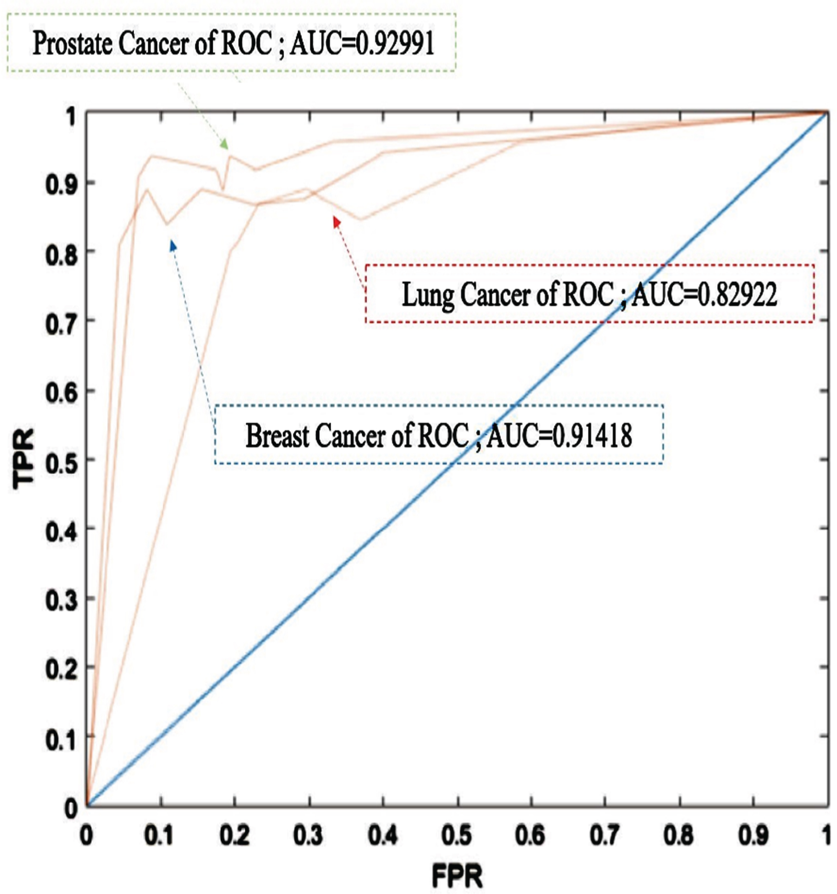
ROC curves comparing with 3 types of cancer detection.

Table 5

Result of Bone scan image with IFV classification

Methods	Sensitivity	Specificity	PPV	NPV	Accuracy
106 male prostate cancer patients (normal:57, meta:49)	93%	92%	91%	89%	90%
162 female breast cancer patients (normal:94, meta:68)	91%	90%	83%	93%	87%
100 lung cancer patients (normal:55, meta:45)	83%	82%	75%	93%	84%

PPV: positive predictive value, NPV: negative predictive value.

The limitations of our study: More cases, further follow-up, and multi-institutional analysis are warranted. Established prognostic factors such as metastatic sites, performance status, and comorbidity index and laboratory data were not included. A few further works may be continued on the proposed approach. Here, a set of possible cases which may be regarded as open and valuable problems to be researched, e.g., (1) To build a database this is suitable for patients in all ages for solving the problem of the limitation for adult only in our algorithm. (2) To develop another analysis algorithm to detect “cold” bone lesion.

5 Conclusions

IFV system was adapted to classify patients ranging from mild symptoms to severe conditions using MRI or CT images. These IFV results were compared with those of manual interpretations and then ML was utilized to perfect IFV to assist the determination of metastasis status and locations. This modified IFV is highly specific and sensitive to support better image interpretation and generate predictions. It can quickly and accurately analyze the lesion threshold values, grayscale distribution and standard deviation. Thus, the proposed machine learning approach in diagnosing bone metastasis may be useful as a decision-support tool.

Funding

This research received no external funding.

Footnotes

Acknowledgments

The authors would like to express their sincere thanks to the anonymous reviewers for their invaluable comments, which have helped to improve the effectiveness of the presentation of this work. The irregular flux viewer (IFV) was provided by Chi-Tsung Chen in support of the self-developed computerized-aided diagnostic software.

Conflicts of interest

The authors declare no conflict of interest.

References

Bray

, Ferlay

, Soerjomataram

, et al., Global cancer statistics: GLOBOCAN estimates of incidence and mortality worldwide for 36 cancers in 185 countries, CA Cancer J Clin 68(6) (2018), 394–424.

McKillop

J.H.

, Bone Scanning in Metastatic Disease, In: Fogelman I. (eds) Bone Scanning in Clinical Practice. Springer, London. (1987).

Sergieva

, Kirova

and Dudov

, Current diagnostic approaches in tumor-induced bone disease, Off J Balk Union Oncol 12 (2007), 493–504.

Abuzallouf

, Dayes

and Lukka

, Baseline staging of newly diagnosed prostate cancer: A summary of the literature, J Urol 171 (2004), 2122–2127.

Bombardieri

and Gianni

, The choice of the correct imaging modality in breast cancer management, Eur J Nucl Med Mol Imaging 31 (2004), S179–S186.

Myers

R.E.

, Johnston

, Pritchard

, et al., Breast Cancer Disease Site Group of the Cancer Care Ontario Practice Guidelines Initiative. Baseline staging tests in primary breast cancer: a practice guideline, CMAJ 164(10) (2001), 1439–1444.

Hendler

and Hershkop

, When to use bone scintigraphy. It can reveal things other studies cannot, Postgrad Med 104 (1998), 54–69.

Müller

, Steinhagen

, de Wit

, et al., Bone scintigraphy in clinical routine, Radiol Oncol 35 (2001), 21–30.

Koizumi

, Wagatsuma

, Miyaji

, et al., Evaluation of a computer-assisted diagnosis system, BONENAVI version 2, for bone scintigraphy in cancer patients in a routine clinical setting, Ann Nucl Med 29 (2014), 138–148.

10.

Huang

J.Y.

, Kao

P.F.

and Chen

Y.S.

, A set of image processing algorithms for computer-aided diagnosis in nuclear medicine whole body bone scan images, IEEE Trans Nucl Sci 54 (2007), 514–522.

11.

Zhang

, Zhao

, Liu

, et al., Multiple metastasis-like bone lesions in scintigraphic imaging, J Biomed Biotechnol 2012 (2012), 957364.

12.

Saha

G.B.

, Fundamentals of Nuclear Pharmacy; Springer: New York, NY, USA, (1997); Volume 4.

13.

Noguchi

, Kikuchi

, Ishibashi

and Noda

, Percentage of the positive area of bone metastasis is an independent predictor of disease death in advanced prostate cancer, Br J Cancer 88 (2003), 195–201.

14.

Doi

, Computer-aided diagnosis in medical imaging: Historical review, current status and future potential, Comput Med Imaging Graph 31 (2007), 198–211

15.

Yin

T.K.

and Chiu

N.T.

, A computer-aided diagnosis for locating abnormalities in bone scintigraphy by a fuzzy system with a three-step minimization approach, IEEE Trans Med Imaging 23 (2004), 639–654.

16.

Peepre

, 99mTc-MDP bone scan in the detection of bone metastases in breast cancer, IOSR J Dent Med Sci 13 (2014), 82–86.

17.

Feng

J.H.

and Gong

J.L.

, Improved gradient vector flow model and its applications, J Numer Methods Comput Appl 31 (2010), 30–38.

18.

and Prince

J.L.

, Snakes, shapes, and gradient vector flow, IEEE Trans Image Process 7 (1998), 359–369.

19.

C.Y.

and Prince

J.L.

, Gradient vector flow deformable models, In Handbook of Medical Imaging; Elsevier: Amsterdam, The Netherlands, (2000).

20.

Zhao

, Zhang

and Yin

, Medical image segmentation based on wavelet analysis and gradient vector flow, J Softw Eng Appl 7 (2014), 1019–1030.

21.

Kohonen

and Honkela

, Kohonen network, Scholarpedia 2 (2007), 1568.

22.

Kohonen

, Self-organized formation of topologically correct feature maps, Biol Cybern 43 (1982), 59–69.

23.

Von Der Malsburg

, Self-organization of orientation sensitive cells in the striate cortex, Boil Cybern 14 (1973), 85–100.

24.

Turing

A.M.

, The chemical basis of morphogenesis, Philos Trans R Soc Lond Ser B Boil Sci 237 (1952), 37–72.

25.

Ultsch

and Siemon

H.P.

, Kohonen’s self-organizing featuremaps for exploratory data analysis, InWidrow, Bernard; Angeniol, Bernard, Proceedings of the International Neural Network Conference (INNC-90), Paris, France, 9–13 July 1990; Kluwer: Dordrecht, The Netherlands, (1990), 305–308.

26.

Ultsch

, U^*-Matrix: A tool to visualize clusters in high dimensional data, Technical Report Nr. 36; Department of Computer Science, University of Marburg: Marburg, Germany, (2003), 1–12.

27.

Ultsch

, Emergence in self-organizing feature maps, In Proceedings of the 6th International Workshop on Self-Organizing Maps (WSOM ’07), Bielefeld, Germany, 3–6 September 2007; Ritter, H., Haschke, R., Eds.; Neuroinformatics Group: Bielefeld, Germany, 2007.

28.

Korn

T.M.

and Korn

G.A.

, Mathematical Handbook for Scientists and Engineers: Definitions, Theorems, and Formulas for Reference and Review, New York: Dover Publications, (2000), 157–160.

29.

Von der Malsburg

, Self-organization of orientation sensitive cells in the striate cortex, Kybernetik 14 (1973), 85–100.

30.

Evangelista

, Panunzio

, Polverosi

, et al., Early bone marrow metastasis detection: The additional value of FDG-PET/CT vs. CT imaging, Biomed Pharmacother 66 (2012), 448–453.

31.

Kikushima

, Hanawa

and Kotake

, Diagnostic performance of bone scintigraphy analyzed by three artificial neural network systems, Ann Nucl Med 29 (2014), 125–131.

32.

Luna

, Vilanova

J.C.

and Alcalá

Mata L.

, Total body MRI in early detection of bone metastasis and its indication in comparison to bone scan and other imaging techniques (only abstract), Arch Esp Urol 68 (2015), 371–390.

33.

Utsunomiya

, Shiraishi

, Imuta

, et al., Added value of SPECT/CT fusion in assessing suspected bone metastasis: Comparison with scintigraphy alone and nonfused scintigraphy and CT 1, Radiology 238 (2006), 264–271.

34.

Mittal

B.R.

, Harisankar

C.N.B.

, Agrawal

and Bhattacharya

, F-18 fluoro-deoxy-glucose and F-18 sodium fluoride cocktail PET/CT scan in patients with breast cancer having equivocal bone SPECT/CT, Indian J Nucl Med 29 (2014), 81–86.

35.

Tarnawska-Pierścińska ŁHołody

, Braziewicz

and Królicki

, Bone metastases diagnosis possibilities in studies with the use of 18F-NaF and 18F-FDG, Nucl Med Rev 14 (2011), 105–108.

36.

Sadik

, Hamadeh

, Nordblom

, et al., Computer-assisted interpretation of planar whole-body bone scans, J Nucl Med 49 (2008), 1958–1965.

37.

Munné

, Alameda

, Bergueiro

, et al., Unusual presentation of endometrial cancer: A clinicopathological study of one case, Open J Obstet Gynecol 5 (2015), 3–27.

38.

Loizzi

, Cormio

, Cuccovillo

, et al., Two cases of endometrial cancer diagnosis associated with bone metastasis, Gynecol Obstet Investig 61 (2006), 9–52.

39.

Papandrianos

, Papageorgiou

, Anagnostis

, andPapageorgiou, Bone metastasis classification using whole body images from prostate cancer patients based on convolutional neural networks application, PLoS ONE 15 (2020), 0237213.

40.

Koizumi

, Motegi

, Koyama

, et al., Diagnostic performance of a computer-assisted diagnostic system: Sensitivity of BONENAVI for bone scintigraphy in patients with disseminated skeletal metastasis is not so high, Ann Nucl Med 34 (2020), 00–211.

41.

Rong

, Ren

, and ing, MRI and bone scintigraphy for breast cancer bone metastasis: A meta-analysis, Open Med 14 (2019), 17–323.

42.

Papandrianos

, Papageorgiou

, Anagnostis

and Feleki , A deep-learning approach for diagnosis of metastatic breast cancer in bones from whole-body scans, Appl Sci 10 (2020), 97.