RICT: Rotating image computed tomography with a one-to-one reversible image rotation algorithm

Abstract

BACKGROUND:

The Mueller, Siddon and Joseph weighting algorithms are frequently used for projection and back-projection, which are relatively complicated when they are implemented in computer code.

OBJECTIVE:

This study aims to reduce the actual complexity of the projection and back-projection.

METHODS:

First, we neglect the exact shape of the pixel, so that its shadow is a rectangle projecting precisely to a detector bin, which implies that all the pixel weights are exactly 1 for each ray through them, otherwise are exactly 0. Next, a one-to-one reversible image rotation algorithm (RIRA) is proposed to compute the projection and back-projection, where two one-to-one mapping lists namely, U and V, are used to store the coordinates of a rotated pixel and its corresponding new coordinates, respectively. For each 2D projection, the projection is simply the column sum in each orientation according to the lists U and V. For each 2D back-projection, it is simply to arrange the projection to the corresponding column element according to the lists U and V. Thus, there is no need for an interpolation in the projection and back-projection. Last, a rotating image computed tomography (RICT) based on RIRA is proposed to reconstruct the image.

RESULTS:

Experiments show the RICT reconstructs a good image that is close to the result of filtered back-projection (FBP) method according to the RMSE, PSNR and MSSIM values. What’s more, our weight, projection and back-projection are much easier to be implemented in computer code than the FBP method.

CONCLUSION:

This study demonstrates that the RIRA method has potential to be used to simplify many computed tomography image reconstruction algorithms.

Keywords

Computed tomography (CT)image reconstruction limited-angle CT reversible image rotation

1 Introduction

At the heart of every digital computed tomography algorithm is a representation of the image being reconstructed, usually a square array of pixels, and “weights” are assigned to each pixel for each ray through it to represent its contribution to the projection of the radiation source onto an array of detector pixels. Gordon [1] considered that each pixel weight is exactly 1 when the centroid of the square pixel is an element of the intersection set of between the square pixel and an x-ray beam (“passage”), otherwise each pixel weight was set to be 0. However, calculating the intersection set is complicated. Peters [2] proposed a fast back projection and reprojection method in computed tomography: the back-projection is implemented by pre-interpolation of the projection data, and then uses nearest-neighbour interpolation to obtain the reconstructed image. The projection is essentially the inverse of the back-projection procedure. Siddon [3] considered computing the weight based on the intersection length of a given ray within the square pixel. The major computation load in a projection operation is to calculate those intersection lengths. Joseph [4] considered a given ray is specified exactly as a straight line, then approximated the projection data by a Riemann sum. Zeng & Gullberg [5] proposed a modified ray-driven method, where the projection is approximated by a weighted sum of other projection data, and their weighting factors are proportional to their lengths of a given ray within the square pixel. De Man and Basu [6] proposed a distance-driven projection and back-projection method, which considered both the detector bin boundaries and the square pixel boundaries are mapped onto the horizontal axis, then the resulting interval lengths are computed as the pixel weights in the projection and back-projection. To provide a simple solution to the problem of assigning a weight to the intersection of a given ray with a square pixel, we recently introduced the Wu antialiasing algorithm [7] as a weighting algorithm for both 2D and 3D CT [8]. These weighting methods are frequently used for projection and back-projection operations, however, they are relatively complicated when implemented in machine code and some interpolation methods are need.

A pixel is supposed to represent a small region of space to the eye. As recognized in designing Retina^© displays [9], we do not really want to see individual pixels. Furthermore, their exact shape does not matter, if we can’t see them individually. This led to the notion that for each projection we could rotate each pixel so that its shadow on the detector array is rectangular rather than a trapezoid, which actually led to some improvement in image quality [10]. We proposed a further generalization based on pointillism art, introducing the notion that the exact shape, position and “color” of a pixel could be varied within reasonable bounds and still produce a good image [11]. To reduce the actual complexity of the projection and back-projection, we neglect the exact shape of the pixel, so that its shadow is a rectangle projecting precisely to a detector bin, it implies that all the pixel weights are exactly 1 for each ray through them, otherwise are exactly 0. It makes that we no need a weighting method to compute the “weight”. Then, this makes the projection and back-projection to be much easier.

One source of problems is simply that the width of detector elements is fixed, at least in all present, inflexible electronics used for image acquisition (cf., however, [12 –14]). So here we introduce a simple notion: let us rotate the pixel array for reconstruction so that each column always projects onto the same detector pixel. This will work for parallel projections. Of course, we do not actually rotate the image. What we rotate is the virtual grid on which the partially reconstructed image is represented. The rotation can be carried out by any of a large number of rotation algorithms of varying accuracy [15 –22]. Other attempts at reversible image rotation have relied on more accurate interpolation [23, 24]. The generalization to fan or cone beams could be made by generalizing rotation algorithms to these geometries via affine projections. Here, for simplicity, and to demonstrate the power of our approach, we will stick with parallel projections, such as were used in the original EMI scanner [25].

Our paper is organized as follows. The existing methods and the newly proposed method are shown in section II. The numerical experimental results of the proposed method for parallel-beam CT are presented in Section III. Discussion and conclusion are given in Section IV.

2 Methods

2.1 Existing methods

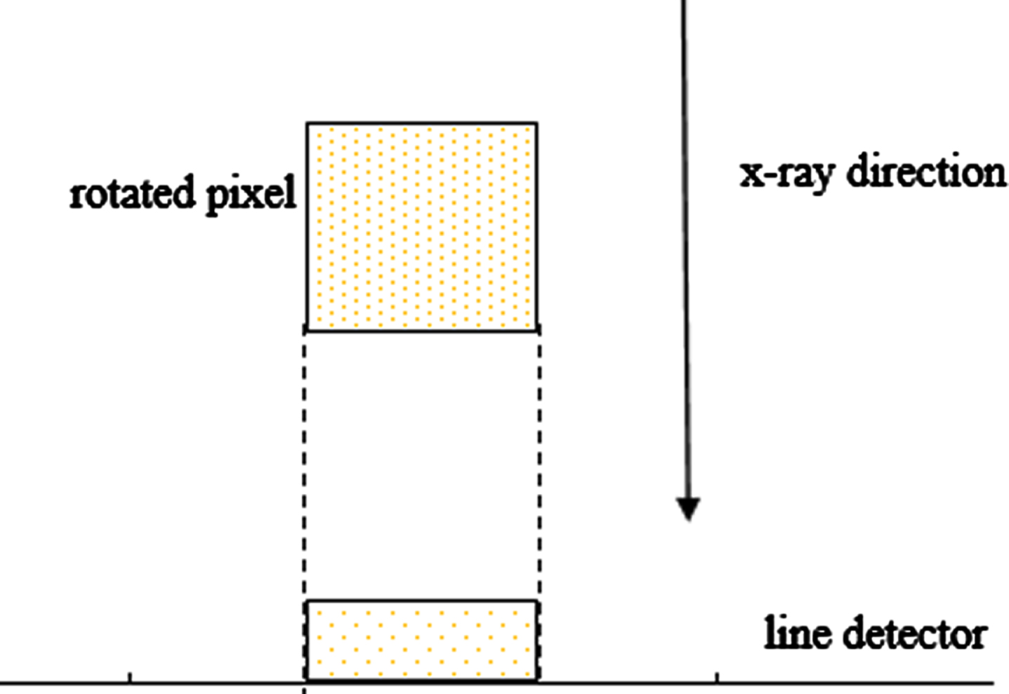
In CT imaging, usually a square array of pixels, and “weights” are assigned to each pixel for each ray through it to represent its contribution to the projection of the radiation source onto an array of detector pixels. A square pixel shadow on the detector array is a trapezoid that overlaps neighboring detectors (see Fig. 1). The pixel shadow changes its shape, from rectangular through trapezoid to triangular, depending on the projection view [10]. The contribution of the pixel to the detectors is involved by assessing how much of the pixel shadow is covered by which of the detectors. To solve this problem, “weights” are assigned to each pixel for each ray through it to represent its contribution to the projection of the radiation source onto an array of detector pixels. For example, the Siddon [3] and Joseph [4] weighting algorithms are frequently used. The Siddon method computes the weight based on the intersection length of a given ray within the square pixel. The Joseph weighting method consideres a given ray is specified exactly as a straight line, then the projection data is approximated by a Riemann sum. We recently introduced the Wu antialiasing algorithm as a weighting algorithm for both 2D and 3D CT [8]. However, for projection and backprojection operations, these weighting methods are relatively complicated when implemented in code and some interpolation methods are need.

Fig. 1

A square pixel’s shadow on a line detector using a parallel beam. While x-rays ordinarily diverge from a nearly point source, parallel rays are available using polycapillary x-ray sources [26].

A pixel is supposed to represent a small region of space to the eye, their exact shape does not matter, if we can’t see them individually. The Interpolative Algebraic Reconstruction Technique (IART) [10] rotates each pixel so that it is aligned with the x-ray direction, so that the pixel’s shadow is of the same rectangular shape regardless of the x-ray direction (see Fig. 2). IART starts by projecting the center of the pixel onto the line of detectors, then a weighting interpolation function, which is shown in the following, was used to represent the pixel contribution to the projection: $g_{i, j} (u) = {\begin{matrix} 1, if | u - P_{i, j} | = 0 \\ 1 - | u - P_{i, j} | if | u - P_{i, j} | \in (0, 1] \\ 0 if | u - P_{i, j} | > 1 \end{matrix}$ (1)

Fig. 2

The pixel shadow on the line detector using the parallel beam with a rotated pixel.

where u is the center of the detector bin and P_i,j is the projection of the centroid of the (i,j) th pixel onto the detector. The results reconstructed by IART are slightly worse than those obtained by using “weights”, but the computation time is shorter.

2.2 The proposed one-to-one reversible image rotation algorithm

Motivated by IART method, to further reduce the actual complexity of the projection and back-projection operations, we neglect the exact shape of the pixel and propose rotating image computed tomography with a one-to-one accurately reversible rotation algorithm. Let us rotate the pixel array for reconstruction so that each column always projects onto the same detector bin, which could be independent of the projection view. Of course, we do not actually rotate the image. What we rotate is the virtual grid on which the partially reconstructed image is represented (see Fig. 3). Unlike the other weighting methods [15 –24], the proposed method does not employ weighted interpolation and considers all the pixel weights are exactly 1 for each ray through them, otherwise they are exactly 0. Thus, the projection is simply the column sum of the image, and the back-projection is correspondingly simple. These operations are now much easier to implement in computer code.

Fig. 3

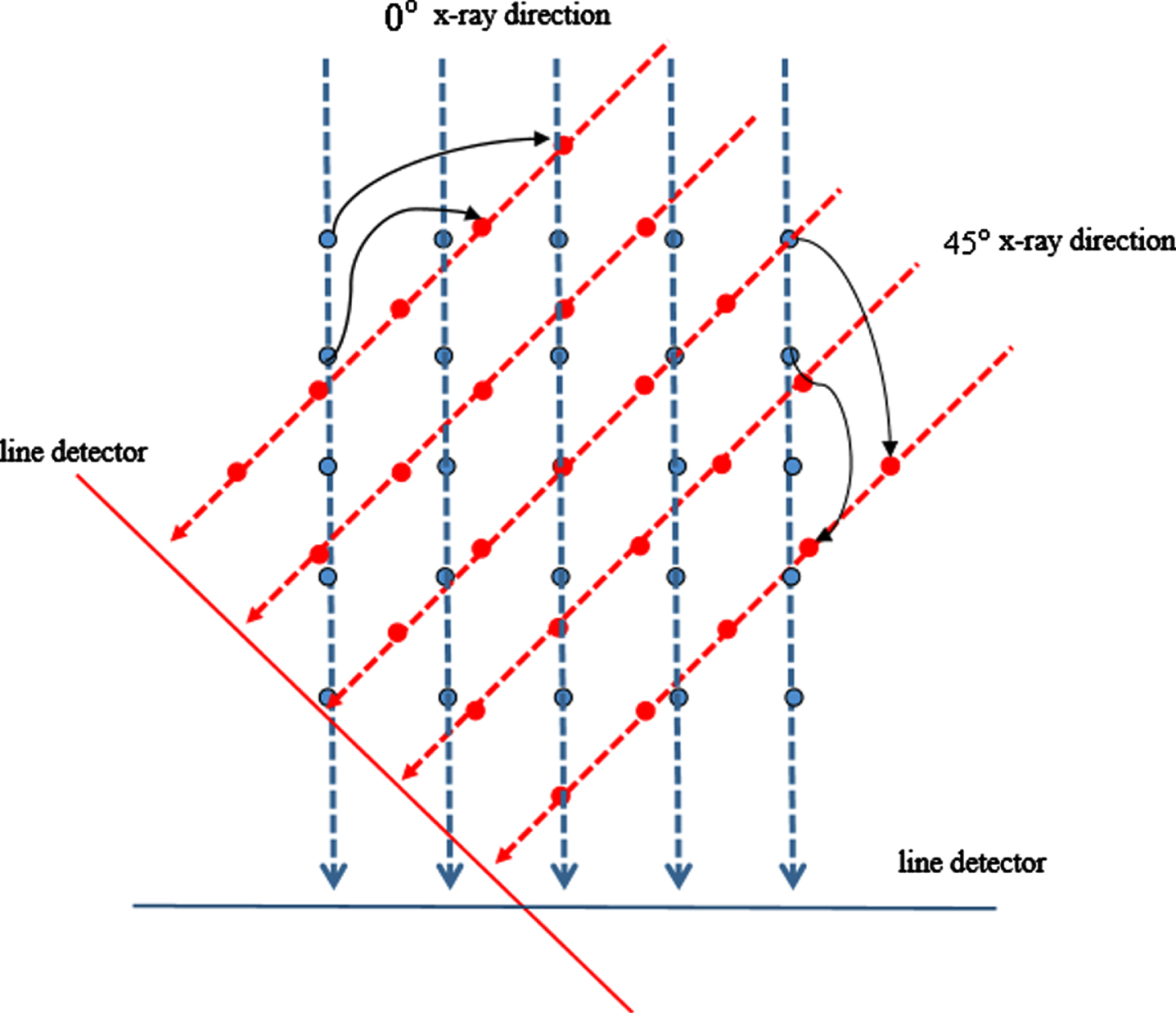
We neglect the exact shape of the pixels and rotate the virtual grid. The blue and red circles are the center of the pixels (i.e., the virtual grids and the rotated virtual grids, respectively). The black curved arrows show the one-to-one corresponding relation of the pixels and the rotated pixels. Each column pixel always projects onto the same detector bin, which could be independent of the x-ray direction, as the bins are rotated with the gantry that holds the x-ray source and detectors, as in most commercial CT scanners.

The value of rotated pixels is crucial to compute the projection and back-projection, these can be carried out by any of a large number of rotation algorithms of varying accuracy, other attempts at image rotation have relied on accurate interpolation [15 –24]. The proposed method does not employ any interpolation and considers all the pixel weights are 1. We find the one-to-one corresponding relation of the pixels and the rotated pixels (see Fig. 3). We use two lists to store the one-to-one mapping for the convenience of computing the projection and back-projection.

The scanned object is placed inside a field of view (FOV) (the red circle of Fig. 4 inscribed in an n×n square image), so that the scanned object is always inside the circle or FOV when we acquire the projection data from different projection views, as in Fig. 4. Thus, we will work with the inscribed circle of an n×n square image in this paper, with the values outside of the inscribed circle set to 0. This is the best configuration for Multiplicative ART (MART) [1 , 27–33].

Fig. 4

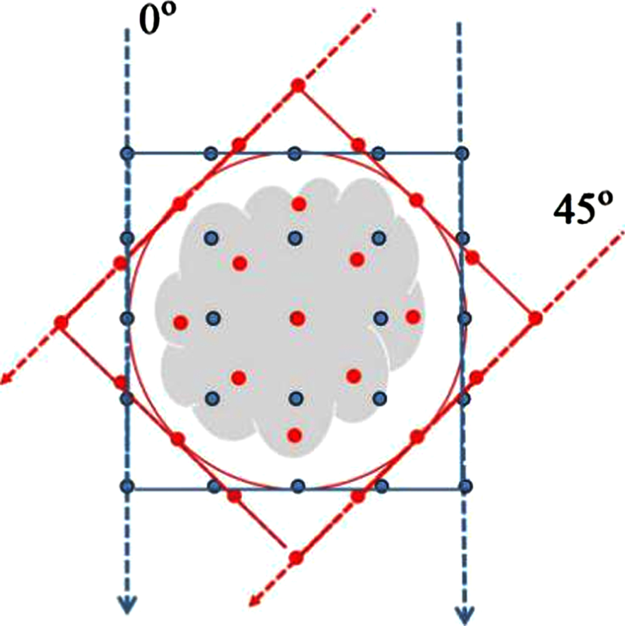
Inscribed circle. The scanned object is always inside the inscribed circle when we acquired the projection data from different projection views.

For an n×n original image or cross section of an object A, let us keep n odd, so there is always a central pixel. Define an integer radius for the inscribed circle r(n) = (n–1)/2. Pixels are numbered 0, 1, . . ., n–1 as their horizontal and vertical coordinates (i,j) The central pixel is at $(\frac{n - 1}{2}, \frac{n - 1}{2})$ . (0,0) is at the lower left-hand corner.

Let D be a mask, that equals to 1 for any pixel that lies within the circle, 0 outside the circle. We will work with D(A). Let D(B) be the result of a rotation, where B is the rotated image with size n×n with the values outside of the inscribed circle set to 0.

As both digital circles inscribing an n×n square image have exactly the same number c(n) of pixels (exact shape of the pixels does not matter), a one-to-one mapping (which is thus reversible) is always possible. There are (c(n))! possible mappings. How do we define which one is best, and how do we explicitly generate the mapping? There are too many to just test them all. Thus, we need a criterion for the best mapping, and an algorithm that generates a mapping that comes close to meeting that criterion.

If we calculate the rotated real value (u,v) of coordinates (i,j) inside D(B), and find the closest pixel (x,y) of (u,v) inside D(A) and store the coordinates (i,j) and its corresponding coordinates (x,y) into two lists U and V, respectively, some pixels inside D(A) will be used twice, so that the map of (i,j) and (x,y) is not a one-to-one mapping. To avoid some pixels inside D(A) being used twice, we first construct a one-to-one mapping rotation algorithm (named as Algorithm I) as follows:

Algorithm I: a one-to-one reversible image rotation algorithm
Input: image A.
Repeat:
1. Choose pixel (i,j) inside D(B) that has not been previously chosen (one can start at (0,0) or spiralling outwards from the center $(\frac{n - 1}{2}, \frac{n - 1}{2})$ );
2. Under a given rotation angle θ, calculate the rotated real value (u,v) of pixel (i,j);
3. Set a label L(x,y) = 0 for all (x,y) inside D(A);
4. If (u,v) falls inside a pixel with integer coordinates (x,y) inside D(A):
a) if L(x,y) = 0, then B(i,j) = A(x,y) and set L(x,y) = 1;
b) if L(x,y) = 1, find the closest pixel (x,y) of (u,v) inside D(A), which was not previously chosen (i.e., the closest pixel with label L(x,y) = 0, then B(i,j) = A(x,y) and set L(x,y) = 1;
5. If (u,v) does not fall inside a pixel with integer coordinates (x,y) inside D(A), find the closest pixel (x,y) of (u,v) inside D(A), which was not previously chosen (i.e., L(x,y) = 0), then B(i,j) = A(x,y) and set L(x,y) = 1;
6. Use two lists U and V to store the coordinates (i,j) and its corresponding new coordinates (x,y), respectively; until all pixels inside D(B) have been handled.
Output: image B.

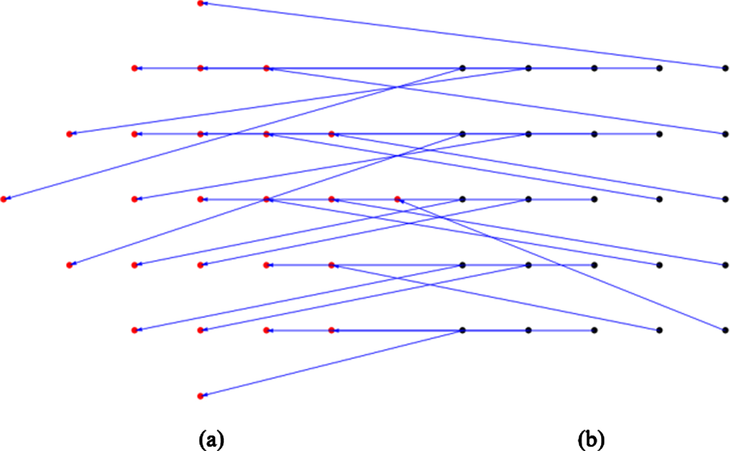
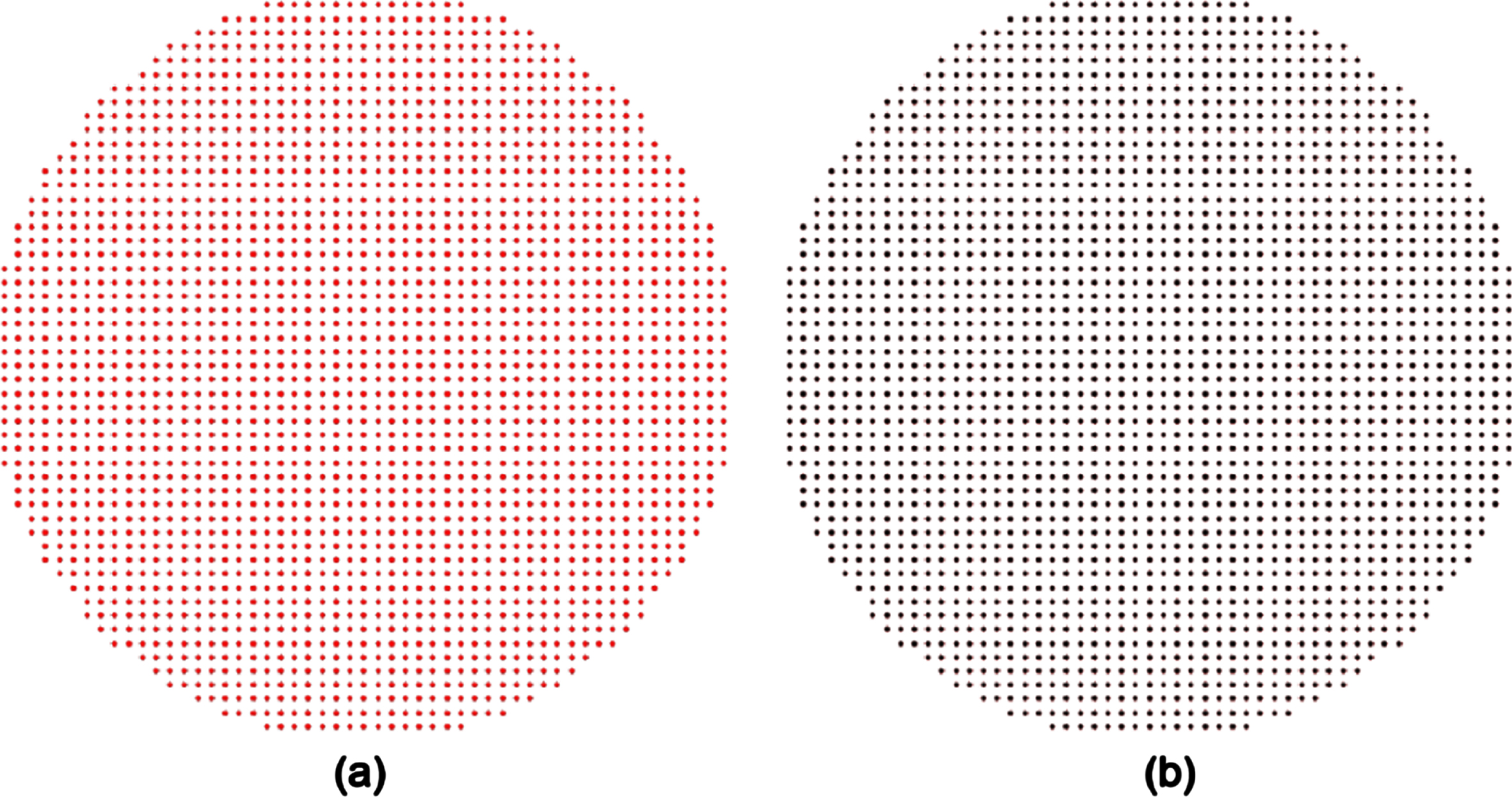
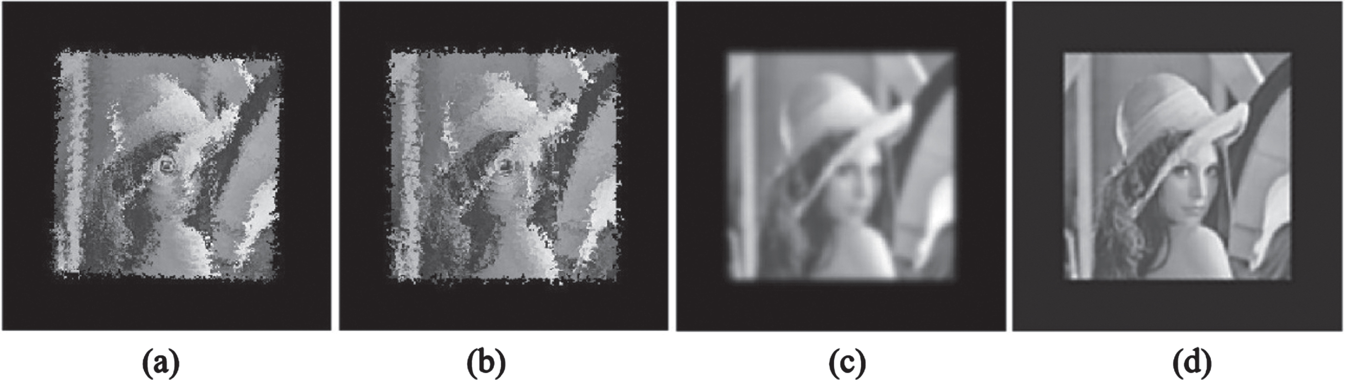
As an example, we choose as an original image that given in Fig. 5a, with size 55×55 pixels, with the white square with of size 25×25 included in the original image, then rotate the original image θ= 40° clockwise. The experimental result of the pixel (i,j), starting at (0,0) using the Algorithm I, is given in Fig. 5b. Figure 6 shows two lists that have stored the (i,j) and its corresponding (x,y), Fig. 6a shows the pixels inside D(A), Fig. 6b shows the pixels inside D(B). We randomly chose a 5×5 neighborhood to show the corresponding relationship between (i,j) and (x,y), and the zoomed-in view is given in Fig. 7. As seen from Figs. 5 , 6 and 7, all pixels inside D(A) are used: it is a one-to-one mapping. However, some pixels near the edge of D(B) of the rotated image are assigned outside values.

Fig. 5

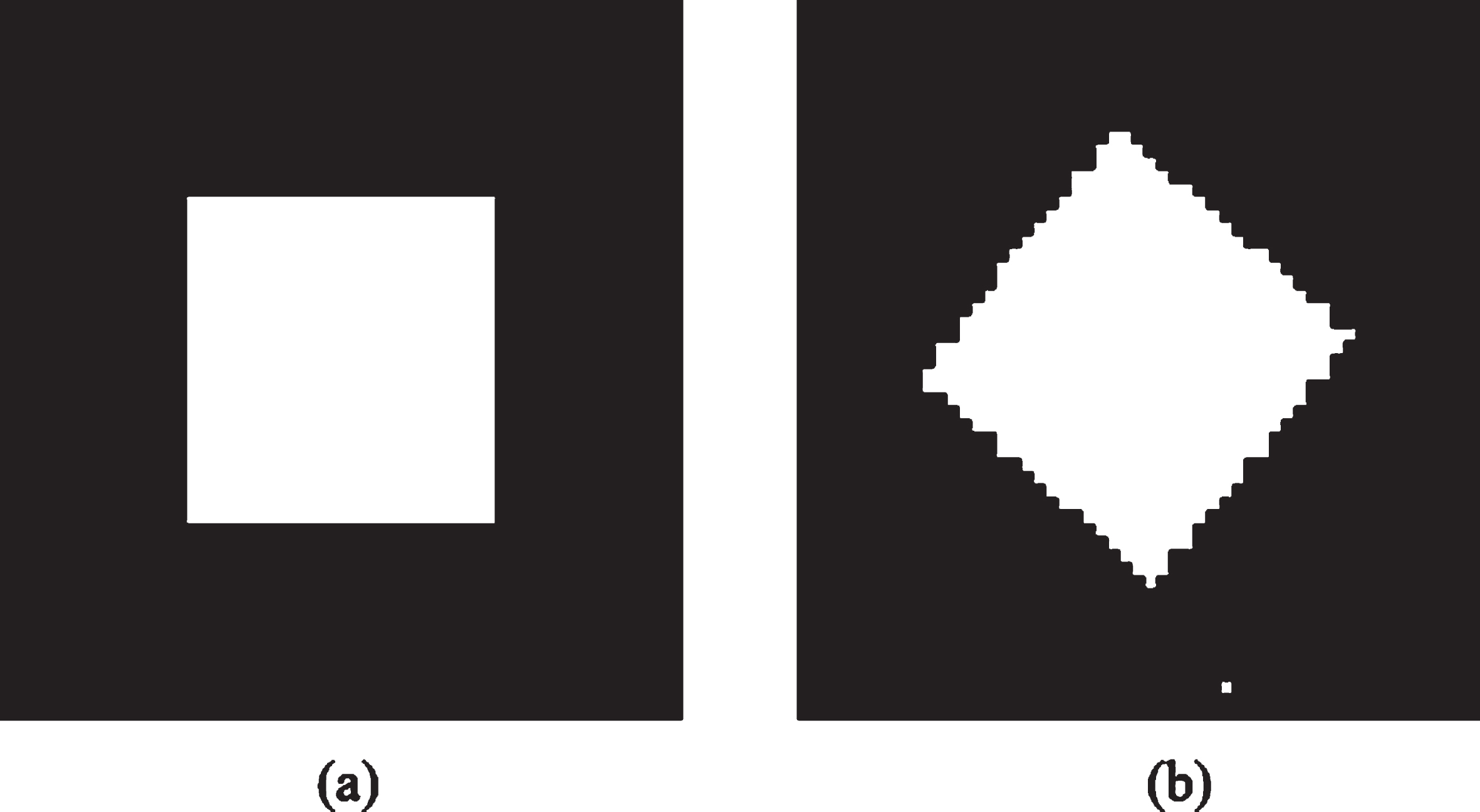
The rotated result. (a) original image; (b) the rotated image B, using Algorithm I.

Fig. 6

Two lists that have stored the (i,j) and its corresponding (x,y). (a) shows the pixels used inside D(A); (b) shows the pixels used inside D(B), using Algorithm I.

Fig. 7

The zoomed-in view of the corresponding relationship between (i,j) and (x,y) of a selected 5×5 neighborhood, using Algorithm I.

The experimental result of the pixel (i,j) as spiraling outwards from the center $(\frac{n - 1}{2}, \frac{n - 1}{2})$ using the Algorithm I is given in Fig. 8b. Figure 9 shows two lists that have stored the (i,j) and their corresponding (x,y). As seen from Figs. 8 9, although we obtain a one-to-one mapping, some pixels near the edge of the rotated image D(B) are assigned outside values.

Fig. 8

The rotated result using the spiral outwards. (a) original image; (b) the rotated image B, using Algorithm I.

Fig. 9

Two lists that have stored the (i,j) and its corresponding (x,y). (a) shows the pixels used inside D(A); (b) shows the pixels used inside D(B), using Algorithm I.

If we want to obtain a one-to-one mapping for all pixels inside D(B), we should find the closest pixel (x,y) of (u,v) inside D(A), then the pixels at the edge of D(B) will be assigned coordinates that belong to the scanned object. We know that the scanned object is always inside the circle. This avoids the problem seen in Figs. 5b 8b showing some weird white blocks at the edge of the inscribed circle. The pixels at the edge of D(B) that are not assigned a value nevertheless have a negligible effect on the CT reconstruction. To avoid the pixels at the edge of D(B) being assigned an outside value, we choose a circular neighborhood to find the closest pixel not previously chosen for (u,v), and set the value of the pixels inside D(B) that cannot find a closest pixel (x,y) inside the circular neighborhood, but find the closest pixel (x,y) inside whole D(A) to 0. The improved one-to-one mapping rotation algorithm (named as Algorithm II) is as follows:

Algorithm II: an improved one-to-one reversible image rotation algorithm
Input: image A.
Repeat:
1. Choose pixel (i,j) inside D(B) that has not been previously chosen (one can start at (0,0) or spiralling outwards from the center $(\frac{n - 1}{2}, \frac{n - 1}{2})$ );
2. Under the given rotation angle θ, calculate the rotated real value (u,v) of pixel (i,j);
3. Set a label L(x,y) = 0 for all (x,y) inside D(A);
4. If (u,v) falls inside a pixel with integer coordinates (x,y) inside D(A);
a) if L(x,y) = 0, then B(i,j) = A(x,y) and set L(x,y) = 1;
b) if L(x,y) = 1, find the closest pixel (x,y) of (u,v) inside a circular neighborhood with radius p (p an odd number), which is not previously chosen (i.e., the closest pixel with label L(x,y) = 0), then B(i,j) = A(x,y) and set L(x,y) = 1;
5. If (u,v) does not fall inside a pixel with integer coordinates (x,y) inside a circular neighborhood with radius p, find the closest pixel (x,y) of (u,v) inside D(A), which was not previously chosen (i.e., L(x,y) = 0), then B(i,j) = A(x,y) and set L(x,y) = 1.
a) If the pixel (i,j) cannot find a closest pixel inside a circular neighborhood with radius p, go to 1
b)If the pixel (i,j) can find a closest pixel inside a circular neighborhood with radius p, go to 6.
6. Use two lists U₁ and V₁ to store the coordinates (i,j) and its corresponding new coordinates (x,y), respectively.
Untill all pixels insideD(B) have been handled.
7. According to the list U₁, for the pixels (i,j) do not find a closest pixel inside a circular neighborhood with radius p, we find the closest pixel (x,y) inside whole D(A) with label L(x,y) = 0, and we not set B(i,j) = A(x,y) but B(i,j) = 0.
8. Use two lists U₂ and V₂ to store the pixels (i,j) and its corresponding new coordinates (x,y) in step 7. Then, U₁,V₁,U₂ and V₂ form two lists U = {U₁, U_} and V = {V₁, V₂}.
Output: image B

According to the Algorithm II, there exist a one to one mapping between the lists U and V, i.e. the pixels inside D(A) have a one to one mapping with regard to the corresponding pixels inside D(B). We know the values of pixels satisfy that B(i,j) = A(x,y) for (i,j) ∈ U₁ and (x,y) ∈ V₁; B(i,j) = 0 for (i,j) ∈ U₂ and (x,y) ∈ V₂. What’s more, the lists U and V are decided by p and θ. The smaller p leads to some pixels inside the scanned object being set to 0. A bigger p makes the pixels at the edge of D(B) be assigned to an outside value that belongs to the scanned object. Generally, we set p = 3 or 5 in Algorithm II to obtain a satisfactory rotated image. Note that algorithm II degenerates into algorithm I if p is large enough.

We choose as an original image that given in Fig. 5a, with size 55×55 pixels, with the white square with of size 25×25 included in the original image, then rotate the original image θ= 40° clockwise. We choose a circular neighborhood with radius p = 3 to find the closest pixel not previously chosen for (x,y). The experimental result of the pixel (i,j) to start at (0,0) or spiraling outwards from the center $(\frac{n - 1}{2}, \frac{n - 1}{2})$ using the Algorithm II is given in Fig. 10b and 10c, respectively. Compared with Figs. 5b and 8b , 10b and 10c show the weird white blocks at the edge of the inscribed circle in Figs. 5b 8b are eliminated.

Fig. 10

The rotated result using the Algorithm II. (a) original image; (b) the rotated image B with the pixel (i,j) to start at (0,0), (c) the rotated image B with the pixel (i,j) spiraling outwards from the center ((n-1)/2, (n-1)/2).

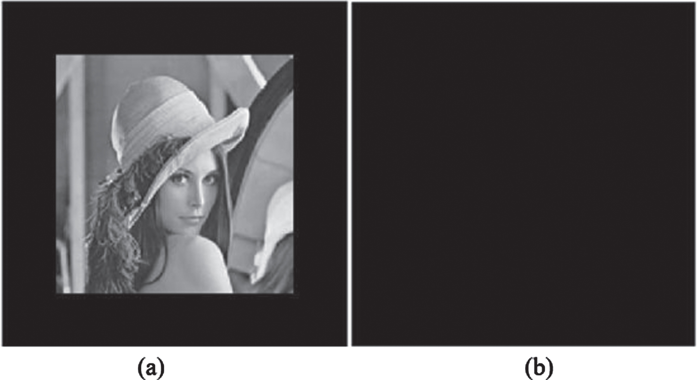
To demonstrate the effectiveness of our Algorithm II for more general image, we use a modified Lena image [34] with size 255×255, then rotate of the original image by θ= 40° clockwise. In our experiments, we choose a circular neighborhood with radius p = 3 to find the closest pixel not previously chosen for (x,y), we show the experimental result with the pixel (i,j) to start at (0,0) in Fig. 11b. We also choose the pixel (i,j) to spiral outwards from the center and the experimental result is given in Fig. 12b. This experimental result shows that the quality of the rotated image is satisfactory.

Fig. 11

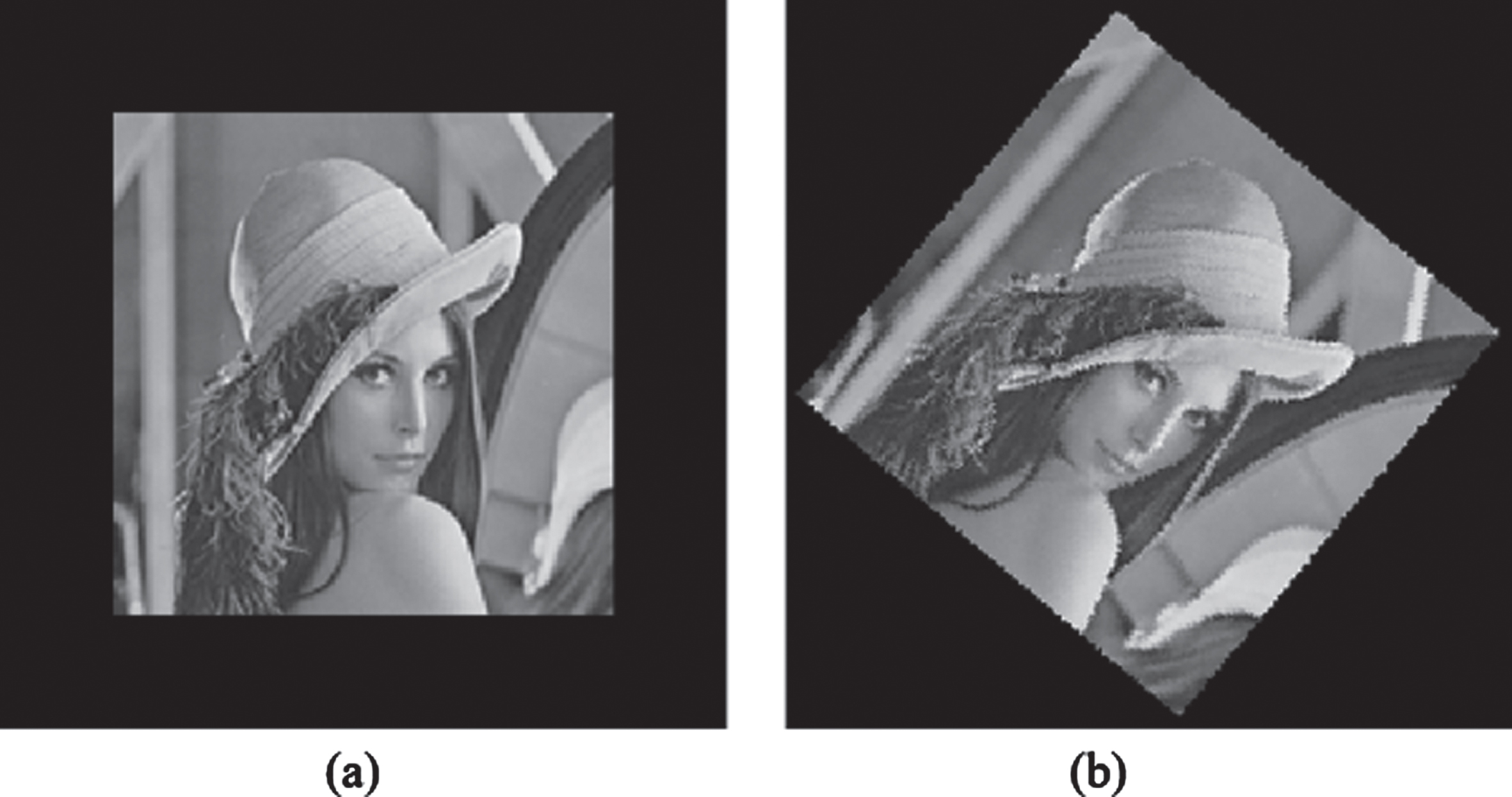
The rotated result with the pixel (i,j) starting at (0,0). (a) original image; (b) the rotated image.

Fig. 12

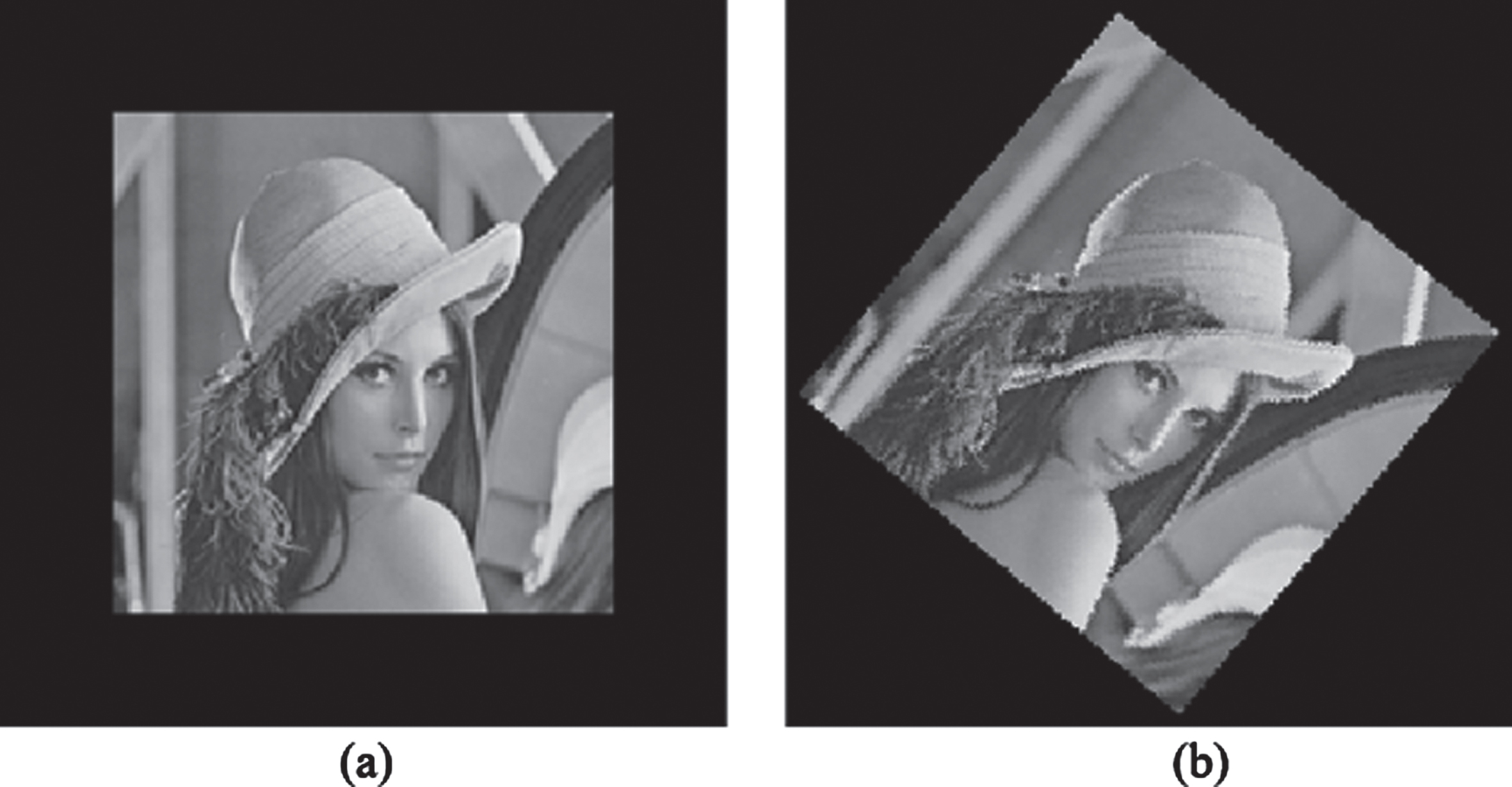
The rotated result using the spiral outwards. (a) original image; (b) the rotated image.

A rotation by 360° should be an identity transformation, resulting in no change to the image. To check if our new rotation algorithm has this property, we compare the original image with its 360° images. Rotations by consecutive rotations of 10° in 36 steps are shown in Fig. 13. From left to right are the results rotated by our rotation method and the built-in rotation algorithm “imrotate” in MatLab with the interpolation method “nearest”, “bilinear” and “bicubic”, respectively. As seen from Fig. 13, using our rotation method, the rotation error will accumulate if the image is rotated by consecutive rotations. Figure 14 shows the rotations of Lena every 30°, each starting from 0 deg, show few losses. Figure 15 shows the rotated result of 360° and the difference image between the rotated image and the original image. It shows that our rotation algorithm has the identity transformation property when we rotate the image 360°.

Fig. 13

Rotations by consecutive rotations of 10° in 36 steps to a full rotation of 360°. (a) our rotation method; (b) MatLab “imrotate” with the interpolation method “nearest”; (c) imrotate with the interpolation method “bilinear”; (d) “imrotate” with the interpolation method “bicubic”.

Fig. 14

Rotations of Lena every 30°, each starting from 0 deg, show few losses.

Fig. 15

(a) shows the rotated result of 360°. (b) the difference image between the rotated image and original image.

Thus, we rotate the original virtual grid on which the original image is represented directly. e.g., if we want to obtain the rotated image with 40°, we rotate the original virtual grid 40° directly, rather than, for instance, rotate the virtual grid in 4 steps of 10° each (the rotate example shown in Figs. 11b 12b).

2.3 The proposed rotating image computed tomography (RICT) based on Algorithm II

We designate rows of the rotated image array as being parallel to the detector array, and columns perpendicular to it, then each column corresponds to one ray. The proposed method considers all the pixel weights are exactly 1 for each ray through them, otherwise are exactly 0. The projection is simply the column sum of rotated pixels, and the backprojection is simply to arrange the filtered projection to the corresponding column element for every projection view. The proposed rotating image computed tomography (RICT) using one-to-one reversible image rotation algorithm, named as RICT, is shown as follows:

Algorithm III: RICT
Input: two lists U and V obtained by Algorithm II for all projection views;
Is there projection dataP:
1. If yes, go to reconstruction process;
2. If no, obtain the simulation projection data P by computing the column sum of rotated pixels of phantom A according to two lists U and V, then go to the reconstruction process.
Reconstruction process:
1. Filtering: obtain the filtered projection P_F using a filter, such as “ram-lak”, “shepp-logan”, “cosine”, etc.;
2. Backprojection: arrange the filtered projection to the corresponding column element for every projection view, and obtain the reconstruction image F according to two lists U and V;
3. Nonnegative: change the negative values of reconstruction image F to 0.
Output: Reconstruction image F.

3 Experimental results

3.1 Simulation experiments

The Shepp-Logan phantom is used to test the power of our proposed RICT method. The scanning range was [0,179°] with increments of 1°, with 255 detector bins, with detector pixel width 1 mm². We choose the pixel (i,j) as spiraling outwards from the center, the phantom and projection data are shown in Fig. 16. Figure 16a is the Shepp-Logan phantom, Fig. 16b is the projection obtained by the Radon transform, Fig. 16c is the projection obtained by the proposed RICT method. While the proposed algorithm uses a detector width that is the same with the reconstruction image width, the Radon transform requires the detector width is bigger than the $\sqrt{2}$ times the reconstruction image width. Thus, the projection data obtained by the Radon transform is thinner than our algorithm if we set the detector width equal to the reconstruction image width.

Fig. 16

The phantom and projection data. (a) Shepp-Logan phantom, (b) Radon transform; (c) Proposed method.

For the projection data obtained by the proposed RICT method, the size of object of Shepp-Logan phantom will be scaled if we do not set the size of reconstruction image to 255 for FBP method (the iradon method in Matlab). This is because the projection data is computed by Algorithm II, which designates rows of the rotated image array as being parallel to the detector array, and columns perpendicular to it, then each column corresponds to one ray. 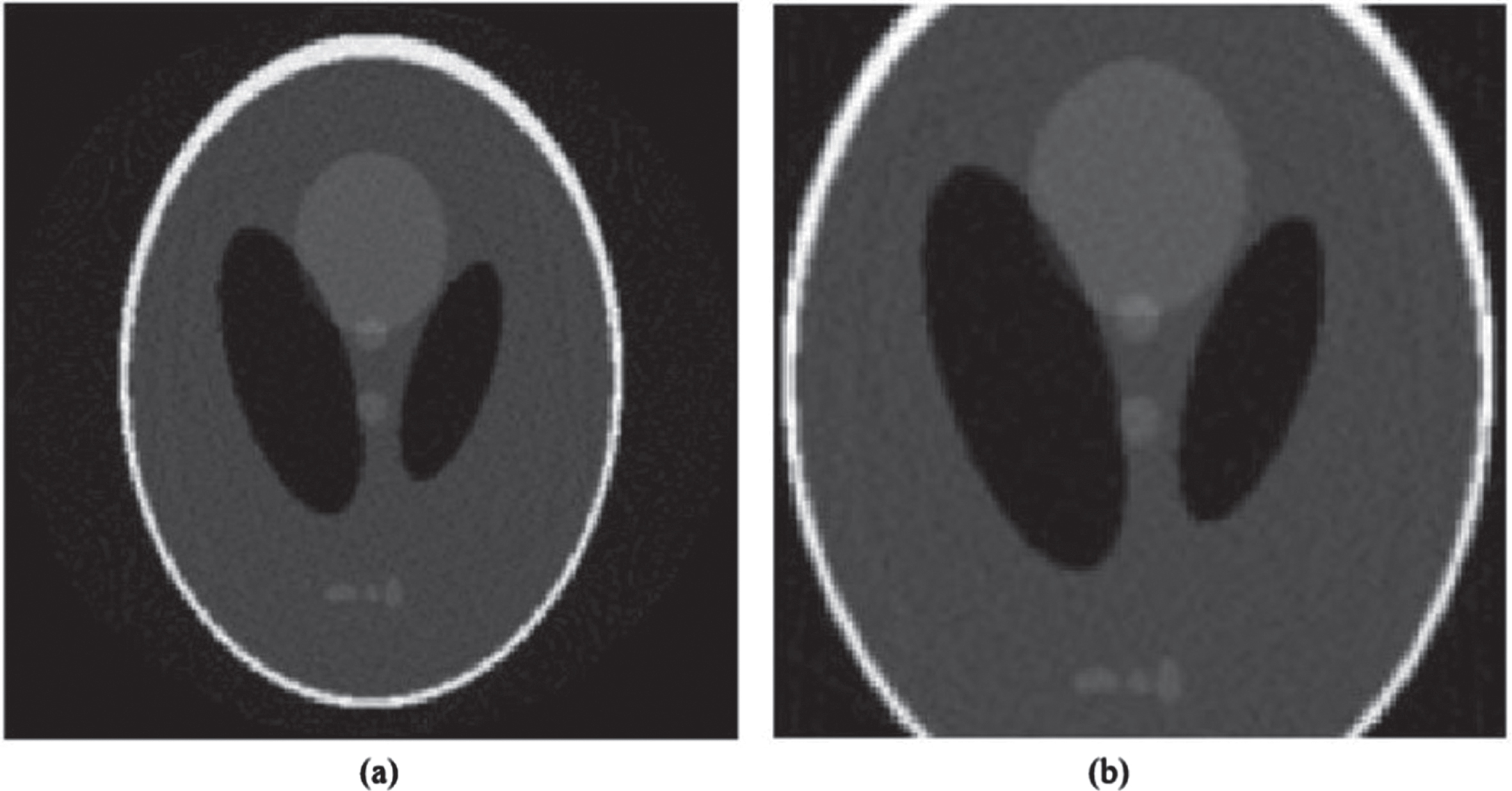However, the size of reconstruction image is computed by $2 \times [\frac{255}{2 \sqrt{2}}] = 180$ for FBP method. Figure 17 shows the results using the proposed RICT method and FBP method, where the “hann” filter is used.

Fig. 17

The results reconstructed by using the proposed RICT method FBP method. (a) the proposed RICT method; (b) FBP method. The display window is [0, 1].

All reconstructed images sizes are 255×255. The results using the proposed RICT method, reconstructed by using different filters, are given in Fig. 18. The results show that the proposed RICT method based on one-to-one reversible image rotation algorithm can approximately reconstruct the image. Compared with the results reconstructed by other three filters, the results reconstructed by the filters “hamming” and “hann” are smoother. The filtered backprojection (FBP) method is also shown for comparison, which is the built-in reconstruction algorithm (iradon) in MatLab. Figure 19 shows the difference images between the reconstructions in Fig. 18 and the original Shepp-Logan phantom. Figure 19 shows the reconstruction result by “hamming” and “hann” filters are closer to the “iradon” reconstruction result with “hann” filter than other three filters.

Fig. 18

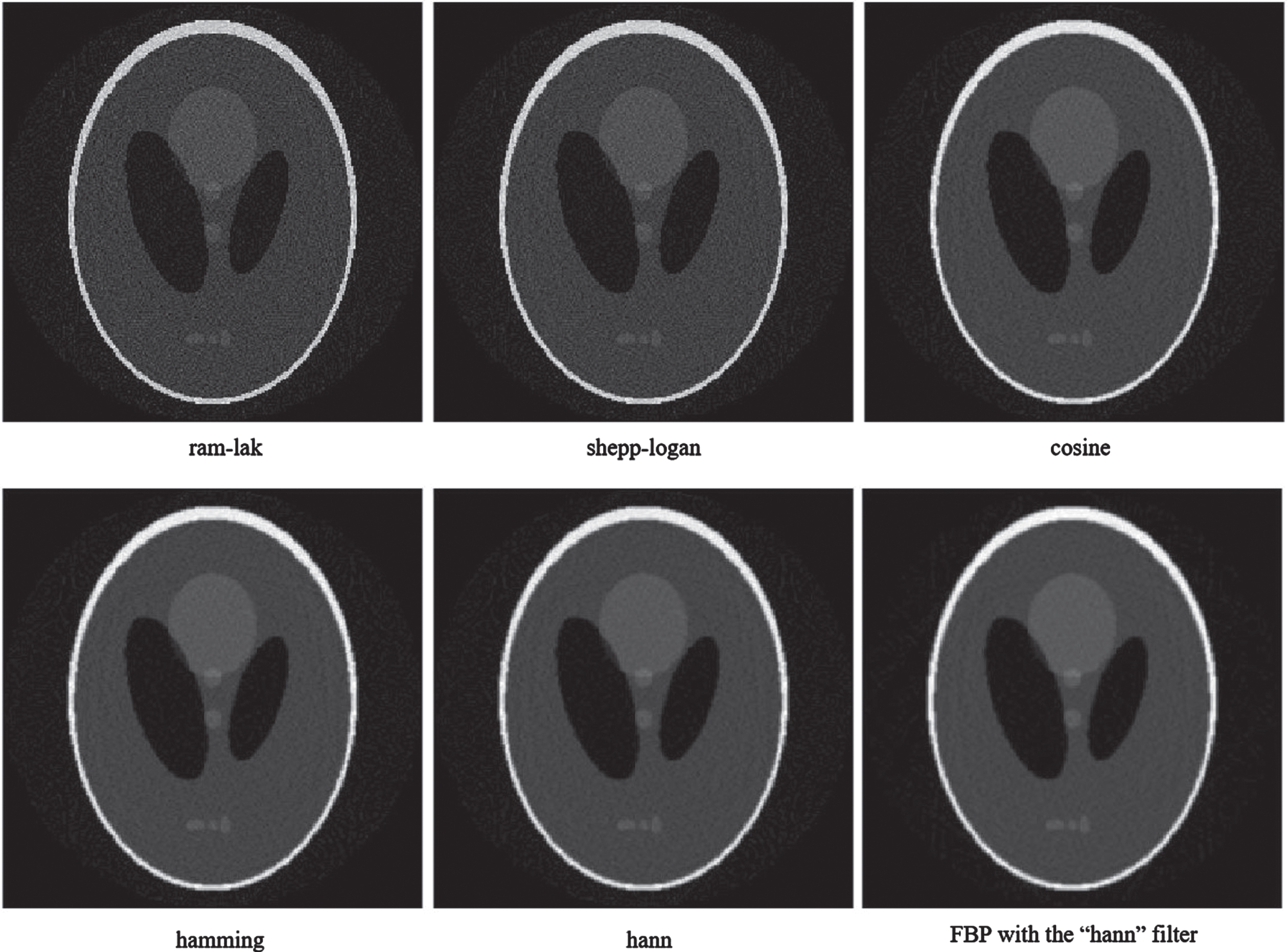
The results reconstructed by using the proposed RICT method with different filters and using the FBP with the “hann” filter. The display window is [0, 1].

Fig. 19

Difference images between the reconstructions in Fig. 18 and the original phantom.

The root mean square error (RMSE) [35], the peak signal-to-noise ratio (PSNR) [35], and the measure of mean structural similarity index (MSSIM) [36] are given in Table 1. From Table 1, we found the filter “shepp-logan” has the minimum RMSE and the maximum PSNR, however the MSSIM value is lower than that obtained by the filters “cosine”, “hamming” and “hann”, and also is lower than that obtained by FBP with “hann” filter. The filter “hann” owns the maximum MSSIM values, but the value of RMSE and PSNR are relatively weak. Considering this in conjunction with Figs. 18 19, we found that the MSSIM value is relatively accurate to evaluate the quality of the reconstructed image.

Table 1

The RMSE, PSNR and MSSIM values of reconstruction image

Filters	ram-lak	shepp-logan	cosine	hamming	hann	FBP-hann
RMSE	0.0513	0.0448	0.0468	0.0514	0.0540	0.0646
PSNR	25.7970	26.9784	26.6019	25.7881	25.3588	23.7990
MSSIM	0.4475	0.5045	0.6639	0.7340	0.7570	0.6535

3.2 Real data experiments

To further test the effectiveness of the proposed RICT method in a practical application, a sufficiently thin slice of Edam cheese, which has been carved with the letters CT, is used. We convert the fan-beam projection data [37] into parallel-beam projection data with a down-sampling factor of 7 in the detector. The parameters of parallel-beam CT are as follows: the projection data is obtained from 319 detectors, the distance from source to rotation center is 403.4 mm, the distance from rotation center to detector is 143.5 mm, the scanning range is [0,179°] with increments of 1°, and the reconstructed image size is 319×319. The results reconstructed by the proposed RICT and FBP methods with “hann” filter are given in Fig. 20. Figure 20 shows the result reconstructed by the proposed RICT method is close to the FBP reconstruction result. This implies that the proposed RICT method using the improved one-to-one reversible image rotation algorithm (Algorithm II) can reconstruct the image closely. The result reconstructed by total variation (TV) minimization method is regarded as the reference image (see Fig. 21), and the RMSE, PSNR, and MSSIM values are given in Table 2. As seen from Table 2, the RMSE, PSNR, and MSSIM values obtained by the proposed RICT method and FBP method are very close.

Fig. 20

The result of carved cheese (placed in open access [37]), reconstructed by the proposed RICT and FBP methods. (a) Proposed RICT method; (b) FBP method. The display window is [0, 0.0143].

Fig. 21

Reference image.

Table 2

The RMSE, PSNR and MSSIM values of reconstruction image

Methods	Proposed RICT	FBP
RMSE	0.0180	0.0181
PSNR	10.0962	10.0828
MSSIM	0.8077	0.8061

Real measurement data of a drumstick, which is obtained from Engineering Research Center of Industrial Computed Tomography Nondestructive Testing of the Education Ministry of China, is used to demonstrate the power of our proposed RICT method. The scanning parameters are given in Table 3. We convert the fan-beam projection data into parallel-beam projection data, then sparse projection data are obtained by two down-sampling factors of 5 and 2 in the detector and projection view, respectively. The projection range is [0,179°]. The size of reconstruction image is 405×405. The results reconstructed by the proposed RICT and FBP methods with “hann” filter are given in Fig. 22. Figure 22 shows the result reconstructed by the proposed RICT method is closer to the FBP reconstruction result.

Table 3

The scanning parameters of the drumstick

Parameters	Values
The distance between rotation center and x-ray source	315.7 mm
The distance between rotation center and detector	879.3 mm
The interval of projection view	0.3519°
The detector bins	2048
The detector pixel	0.2 mm²

Fig. 22

The result reconstructed by the proposed RICT and FBP methods. (a) Proposed RICT method; (b) FBP method. The display window is [0, 0.016].

The result reconstructed by the TV minimization method is regarded as the reference image (see Fig. 23), and the RMSE, PSNR, and MSSIM values are given in Table 4. As seen from Table 4, the PSNR, and MSSIM values obtained by the FBP method are slightly higher than that obtained by the proposed RICT method, but they are very close.

Fig. 23

Reference image.

Table 4

The RMSE, PSNR and MSSIM values of reconstruction image

Methods	Proposed RICT	FBP
RMSE	0.0089	0.0089
PSNR	17.3081	17.3192
MSSIM	0.8961	0.8963

4 Discussions and conclusions

In some CT reconstruction methods, the Mueller, Siddon and Joseph weighting algorithms are frequently used for projection and back-projection, which are relatively complicated when implemented in computer code. To reduce the actual complexity of the projection and back-projection, we firstly neglect the exact shape of the pixel, so that its shadow is a rectangle projecting precisely to a detector bin, it implies that all the pixel weights are exactly 1 for each ray through them, otherwise are exactly 0. Secondly, a one-to-one reversible image rotation algorithm (RIRA) is proposed to compute the projection and back-projection, where two one-to-one mapping lists U and V are used to store the coordinates of a rotated pixel and its corresponding new coordinates, respectively. For each 2D projection, the projection is simply the column sum in each orientation according to the lists U and V. For each 2D back-projection, it is simply to arrange the projection to the corresponding column element according to the lists U and V. There is no need for an interpolation in the projection and back-projection. Lastly, a rotating image computed tomography (RICT) based on RIRA is proposed to reconstruct the image. The filtered backprojection filter “hann” may be the best computed tomography (CT) filter for our proposed RICT method in terms of the quality of the reconstruction image. According to the reconstruction results, the proposed RICT with a one-to-one accurately reversible rotation method (Algorithm II) can reconstruct the image reasonably well, and which is close to the FBP reconstruction result. However, our weight, projection and back-projection are much easier to be implemented in computer code than the FBP method. For CT, the projection and back-projection of RICT could be used in any other iterative CT algorithm, further experiments are needed with iterative CT algorithms. And we use two lists to store the one-to-one mapping for the convenience of the compute of the projection and back-projection. These two lists can be repeated used for fixed scanning geometry to reduce calculation amount. The proposed RICT with its one-to-one accurately reversible rotation method (Algorithm II) is universally applicable.

Large number of refinements could be envisaged, due to the huge combinatorics of pixel assignment from an image to its rotated image (c (n))!. For example, ray sums along a given column are not changed by switching pixels in that column. Switching criteria could be based on sorting on similarity of a pixel to its nearest neighbors [4]. A pair of pixels could be switched if their new locations resulted in a better match to nearest neighbors, perhaps with lower probability if they are far apart. If we keep track of the switches, the algorithm remains reversible. Thus, we do not claim that our one-to-one accurately reversible rotation method (Algorithm II) is the best achievable, but only a starting point for further research. It is generalizable to rotation of 3D images.

Footnotes

Acknowledgments

This work was funded by the National Natural Science Foundation of China (NSFC) (No. 61801086); Natural Science Foundation of Chongqing (No. cstc2019jcyj-msxmX0345); Science and technology research program of Chongqing Education Commission of China (No. KJQN202000534); Scientific Research Funds of Chongqing Normal University (19XLB005). The librarians of Wayne State University and the University of Manitoba are thanked for obtaining many references.

References

Gordon

, A tutorial on ART (Algebraic Reconstruction Techniques) [Erratum in Eq. 18: max, not min], IEEE Transactions on Nuclear Science NS-21 (1974), 78–93, 95.

Peters

T.M.

, Algorithms for fast back and re-projection in computed tomography, IEEE Transactions on Nuclear Science 28(4) (1981), 3641–3647.

Siddon

R.L.

, Fast calculation of the exact radiological path for a three-dimensional CT array, Medical Physics 12(2) (1985), 252–255.

Joseph

P.M.

, An improved algorithm for reprojecting rays through pixel images, IEEE Transactions on Medical Imaging 1(3) (1982), 192–196.

Zeng

G.L.

and Gullberg

G.T.

A ray-driven backprojector for backprojection filtering and filtered backprojection algorithms, in Nuclear Science Symposium and Medical Imaging Conference (NSS-MIC 93). 1993, IEEE: San Francisco, Ca. p. 1199–1201.

De Man

and Basu

, Distance-driven projection and backprojection, in IEEE Nuclear Science Symposium/Medical Imaging Conference (NSS/MIC), 2002, IEEE: Norfolk, Va. p. 1477–1480.

X.L.

, An efficient antialiasing technique, SIGGRAPH 91 Conference Proceedings 25 (1991), 143–152.

Alvare

and Gordon

, Foxels for high flux, high resolution computed tomography (FoxelCT) using broad x-ray focal spots: theory and two-dimensional fan beam examples, Radiology and Diagnostic Imaging 1(1) (2017). doi: 10.15761/RDI.1000103

Hemphill

, What is a Retina display? 2018; Available from: https://www.macworld.com/article/670709/what-is-a-retina-display.html

10.

Mazur

E.J.

and Gordon

, Interpolative algebraic reconstruction techniques without beam partitioning for computed tomography, Medical & Biological Engineering & Computing 33(1) (1995), 82–86.

11.

Gordon

, Stop breast cancer now! Imagining imaging pathways towards search, destroy, cure and watchful waiting of premetastasis breast cancer, in Breast Cancer – A Lobar Disease, T. Tot, Editor. 2011, Springer: London. p. 167–203.

12.

Narayanaswamy

M.R.

and Halsmer

M.A.

, Detector array transmission circuit for e.g. x-ray imaging system, has substrate layer coupled to detector, and flexible circuit layers to direct x-ray signals produced by detector to data acquisition system [patent US2005018810-A1; DE102004035405-A1; JP2005040610-A; US7010088-B2; IL162905-A; JP4502736-B2]. 2005: Ge Medical Systems Global Technology Co (Gene-C) Ge Medical Systems Global Technology Co (Gene-C) Ge Medical Systems Global Technology Co (Gene-C) General Electric Co (Gene-C).

13.

Heo

D.C.

, et al., Manufacture of flexible x-ray detector used in radiation detection assembly, involves obtaining image sensor array on auxiliary substrate, preparing flexible substrate, forming electrode lines, and connecting with auxiliary substrate [patent KR2014067257-A; KR1420250-B1]. 2014: Korea Electrotechnology Res Inst (Koel-C).

14.

Miao

J.L.

and Zhang

F.J.

, Recent progress on highly sensitive perovskite photodetectors, Journal of Materials Chemistry C 7(7) (2019), 1741–1791.

15.

Cambridge in Colour, Digital Image Interpolation, 2020 December 18, 2021]; Available from: https://www.cambridgeincolour.com/tutorials/image-interpolation.htm

16.

Kwon

H.-C.

and Kwon

, Image rotation using an augmented 2-step shear transform, World Academy of Science, Engineering Technology, International Journal of Computer, Electrical, Automation, Control Information Engineering 11(1) (2017), 60–63.

17.

Ashtari

A.H.

, Nordin

M.J.

and Kahaki

S.M.M.

, Double line image rotation, IEEE Transactions on Image Processing 24(11) (2015), 3370–3385.

18.

Paeth

A.W.

, A fast algorithm for general raster rotation, in Proceedings Graphics Interface 86 May 26–30, 1986, Vancouver, British Columbia, Canada, 1986, Canadian Human-Computer Communications Society, p. 77–81.

19.

Parker

J.A.

, Kenyon

R.V.

and Troxel

D.E.

, Comparison of interpolating methods for image resampling, IEEE Transactions on Medical Imaging 2(1) (1983), 31–39.

20.

Meijering

E.H.W.

, Niessen

W.J.

and Viergever

M.A.

, Quantitative evaluation of convolution-based methods for medical image interpolation, Medical Image Analysis 5(2) (2001), 111–126.

21.

Di Bella

E.V.R.

, et al., A comparison of rotation-based methods for iterative reconstruction algorithms, IEEE Transactions on Nuclear Science 43(6) (1996), 3370–3376.

22.

Unser

, Thevenaz

and Yaroslavsky

L.J.I.T.

, Convolution-based interpolation for fast, high-quality rotation of images, 4(10) (1995), 1371–1381.

23.

Srinivasan

, Reversible image rotations with modulo transforms, in 2005 International Conference on Image Processing, 2005, IEEE: New York, NY, USA. p. 1629–1632.

24.

Condat

and Van De Ville

, Fully reversible image rotation by 1-D filtering, in 2008 15th IEEE International Conference on Image Processing, Vols1–5 (2008), 913–916.

25.

Hounsfield

G.N.

, EMI scanner, Proceedings of the Royal Society B-Biological Sciences 195 (1977), 281–289.

26.

Jagodzinski

, et al., Properties of polycapillary optics dedicated to low-energy parallel-beam wavelength-dispersive spectrometers for synchrotron-based X-ray fluorescence study, Optics Express 29(17) (2021), 27193–27211.

27.

Bellman

S.H.

, et al. ART is science, being a defense of Algebraic Reconstruction Techniques for three-dimensional electron microscopy, Journal of Theoretical Biology 32 (1971), 205–216.

28.

Zeng

, He

and Liu

, GPU-accelerated MART and concurrent cross-correlation for tomographic PIV, Experiments in Fluids 63 (2022), 91.

29.

Mailloux

G.E.

, et al., The MART algorithm for SPECT and entropy maximization, Proceedings of the SPIE 1887 (1993), 40–49.

30.

Badea

C.T.

, MART vs FBP with angular undersampling for cardiac imaging, 2005.

31.

Mishra

, Muralidhar

and Munshi

, A robust MART algorithm for tomographic applications, Numerical Heat Transfer Part B-Fundamentals 35(4) (1999), 485–506.

32.

Das

S.K.

and Shukla

A.K.

, Two-dimensional ionospheric tomography over the low-latitude Indian region: An intercomparison of ART and MART algorithms, Radio Science 46 (2011).

33.

Colquhoun

G.D.

and Gordon

, The use of control angles with MART (Multiplicative Algebraic Reconstruction Technique), Technology in Cancer Research and Treatment 4(2) (2005), 183–184.

34.

Van Tassel

, The legend of Lena: image processing’s main squeeze, Advanced Imaging 11(5) (1996), 56–60.

35.

Zhang

, Dong

and Lu

, l₀ minimization for wavelet frame based image restoration, Mathematics of Computation 82 (2013), 995–1015.

36.

Wang

, et al., Image quality assessment: From error visibility to structural similarity, Image Processing, IEEE Transactions on 13 (2004), 600–612.

37.

Bubba

T.A.

, et al., Tomographic X-ray data of carved cheese, 2017 December 18, 2021]; Available from: https://arxiv.org/abs/1705.05732, http://www.fips.fi/dataset.php#cheese